Assessment of Streamflow from EURO-CORDEX Regional Climate Simulations in Semi-Arid Catchments Using the SWAT Model

Abstract

This research studies the effect of climate change on the hydrological behavior of two semi-arid basins. For this purpose, the Soil and Water Assessment Tool (SWAT) model was used with the simulation of two future climate change scenarios, one Representative Concentration Pathway moderate (RCP 4.5) and the other extreme (RCP 8.5). Three future periods were considered: close (2019–2040), medium (2041–2070), and distant (2071–2100). In addition, several climatic projections of the EURO-CORDEX model were selected, to which different bias correction methods were applied before incorporation into the SWAT model. The statistical indices for the monthly flow simulations showed a very good fit in the calibration and validation phases in the Upper Mula stream (NS = 0.79–0.87; PBIAS = −4.00–0.70%; RSR = 0.44–0.46) and the ephemeral Algeciras stream (NS = 0.78–0.82; PBIAS = −8.10–−8.20%; RSR = 0.4–0.42). Subsequently, the impact of climate change in both basins was evaluated by comparing future flows with those of the historical period. In the RCP 4.5 and RCP 8.5 scenarios, by the end of the 2071–2100 period, the flows of the Upper Mula stream and the ephemeral Algeciras stream will have decreased by between 46.3% and 52.4% and between 46.6% and 55.8%, respectively.

1. Introduction

Climate change has become one of the main challenges of the 21st century, with a great effort being made to evaluate and analyze its impact on the hydrological cycle [1,2,3]. According to all climatic scenarios, the annual average precipitation will increase in Northern Europe and decrease in the southern Mediterranean regions [4]. Episodes of intense precipitation will be more frequent during the 21st century, increasing the risk of floods in urban centers; in contrast, in arid and semi-arid regions, periods of drought will be more persistent and prolonged [5,6,7], and there will be an increase in the duration and frequency of thermal anomalies, especially heatwaves.

As a measure to mitigate and reduce the risks and impacts of climate change, the governments participating in the COP21 in Paris (2015) set a long-term objective of keeping the increase in world temperature below 2 °C.

Spain is among the countries most vulnerable to the effects of climate change, due to the high spatial and temporal irregularity of its water resources [8]. According to reports prepared by the State Meteorological Agency [9], the average temperature in Spain has increased by 1.7 °C since pre-industrial times, 0.6 °C above the global temperature rise of the planet (1.1 °C). Since 1970, each decade has been warmer than the last. In the Segura River basin this situation is more serious, as it is a region with high spatial and temporal pluviometric variability, which makes it especially sensitive to global atmospheric warming. The northwestern part registers average annual values of precipitation (1000 mm) and temperature (10 °C) that contrast with those observed in the coastal zone (200 mm and 18 °C, respectively). Most of this region is dominated by semi-arid conditions, and the average annual rainfall does not exceed 375 mm while the potential evapotranspiration (PET) exceeds 850 mm/year [10,11], making it particularly vulnerable to the effects of climate change in the short- and medium-term. Various hydrological studies have already revealed the reduction in the water resources derived from climate change in this region [12,13]. In addition, the increase in both the water temperature and the rainfall intensity could trigger the appearance of various types of water pollution (sediments, nutrients, dissolved organic carbon, pesticides, salt, etc.), causing severe ecological crises. This was the case of the torrential episodes caused by the Isolated Depression at High Levels (DANA) during 13–14September 2019 in La Manga del Mar Menor, which discharged between 60 and 70 hm³ of water, with a major anoxia event in a saltwater lagoon [14]. The areas that have experienced the greatest increase in temperature, within the Segura River basin District (DHS), are the interior Neogene Quaternary depressions. Among them, it is worth highlighting the Upper Mula and Algeciras basins, where the average annual temperature rose by 1.1 and 1.3 °C, respectively, during the period of 1972 to 2019. These are semi-arid basins, drained by intermittent and ephemeral water courses, which are witnessing significant changes in their hydrological regimes. The dry channel stages are increasingly prolonged in time and the frequency of flash floods is tending to increase, along with the geomorphological repercussions that this implies [5].

In order to assess these effects in both basins, we used the Soil and Water Assessment Tool (SWAT), calibrated and validated based on the data for the water input received by their respective reservoirs and the temporal changes in the real and potential evapotranspiration values.

This study is therefore part of the recent line of research based on the application of the SWAT model to assess the impact of climate change on water resources in environmentally fragile basins with high water stress (arid and semi-arid regions).

Unlike at the global scale [15], this tool has not yet been sufficiently tested in hydrological and climate change studies regarding this type of semi-arid environment, where there is often great uncertainty due to the lack of continuous gauging data and the difficulty in adopting downscaling methods to produce climate scenarios at the basin scale from Atmosphere Ocean General Circulation Models (AOGCM). However, there have already been some attempts to use SWAT to evaluate the changes in the stream discharge and reservoir inflow of semi-arid and arid basins according to different regional climate change scenarios, such as those performed by Zahabiyoun et al. [16] in the Gharesou basin in Iran or by Shimola and Muthiah [17] in the Vaippar basin in the southern part of Tamil Nadu. In the DHS, where the study areas (the Upper Mula and Algeciras basins) are located, the SWAT model has already been applied by Senent-Aparicio et al. [12] and Jódar-Abellán et al. [13] to assess the effects of climate change on the main components of the water balance in the headwaters of the Segura River basin.

In our case, two semi-arid basins with different lithological characteristics (the Upper Mula headwaters area is mainly composed of limestone and dolomite; and the Algeciras catchment is dominated by marls) were the object of study for two reasons. First, data series are available for the daily average flow (m³/s) of the entry into the La Cierva and Algeciras reservoirs, corresponding to the periods from 1993–2018 and from 2003–2018, respectively, which allowed the SWAT calibration process to be performed. Second, they are basins with different ephemeral hydrological regimes: the Algeciras stream is an ephemeral stream and the Upper Mula is a transitional watercourse with a dry channel almost all year round except when groundwater provides enough water for stream flow—thus, it is between an ephemeral and a seasonal intermittent stream. In this work, the evaluation of the extent to which said differentiation will decrease or disappear with climate change in the short and medium term constitutes a complementary objective of undoubted interest.

The calibration and validation processes were carried out by simulating two future climate change scenarios, one moderate (RCP 4.5) and the other extreme (RCP 8.5). In both cases, three future periods were considered—close (2019–2040), medium (2041–2070), and distant (2071–2100)—and all of them were evaluated with respect to their respective reference periods, 1993–2018 for the Upper Mula basin and 2003–2018 for the Algeciras basin.

2. Materials and Methods

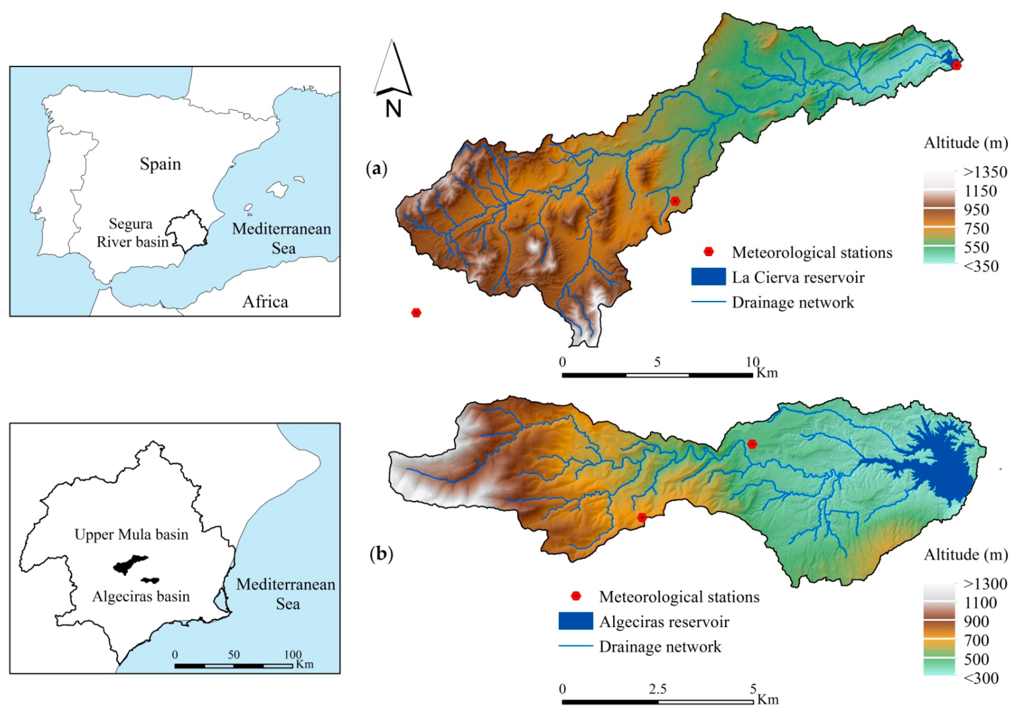
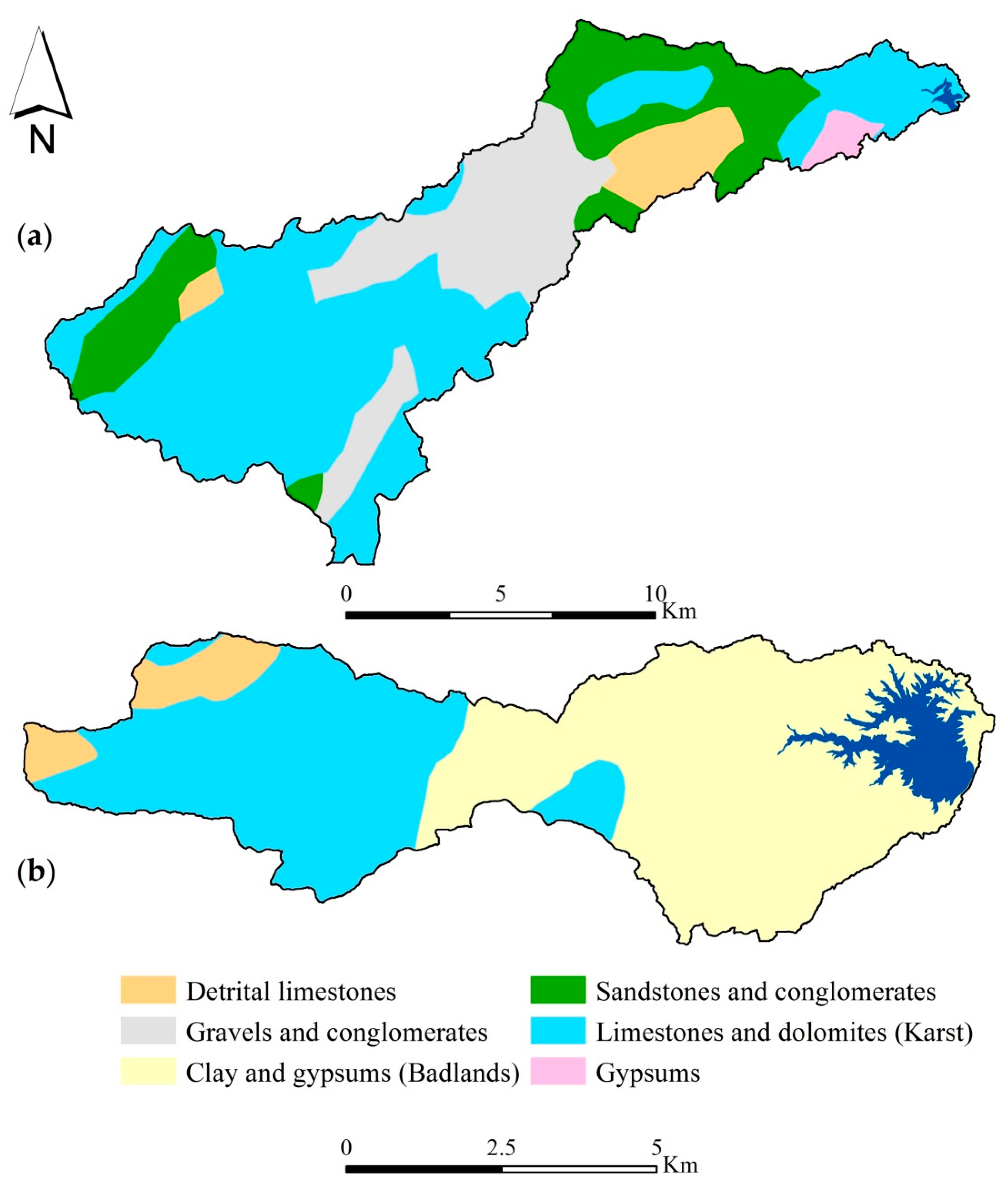
2.1. Study Site

The study areas selected were the Upper Mula stream and the ephemeral Algeciras stream, both located in southeastern Spain (Segura River basin) (Figure 1).

The Upper Mula stream basin covers an area of 169 km², and its main channel is a tributary of the Segura River, while the ephemeral Algeciras stream basin covers an area of 44.9 km² and is drained by the ephemeral Algeciras stream, a dry tributary course of the Guadalentín stream, which is a main tributary of the Segura River. Geologically, they belong to the domain of units in the Betic and Subbetic zone. The limestone and dolomite from the Lías, siliceous marls from Malm, and marly limestone from the Dogger outcrops predominate in the headwaters, while the middle and lower parts of the basin abound with marls from the Upper Miocene with a predominance of badlands relief (Figure 2). The Upper Mula stream is born from the confluence of several gullies and ravines that drain from the Burete, Lavia, and Cambrón mountains.

The mean altitude of the basin (719 m) masks an important contrast between the highlands and the lowlands, with their maximum and minimum altitudes being 1392 m and 232 m, respectively. It includes three large hydrogeological units (HU): the Lower Quipar, Bullas, and Sierra Espuña, which are home to a total of six aquifers. The ephemeral Algeciras stream (15 km in length) starts in the Valdeparra gully. Due to the predominance of loamy soils, with little or no cementation, to the orographic variation (altitudes between 200 and 1320 m), and to the great torrential rains, its watershed has a dense drainage network, mainly formed by gullies and ravines (badlands), which produce, in stormy weather, high rates of erosion and large peak flows (113 m³/s in October 1972).

Both basins have an elongated shape and semi-arid climatic features, marked by low annual rainfall, an irregular rainfall regime, and torrential rains. Both are characterized by a pluviometric gradation, the annual rainfall being 329 mm in the La Cierva reservoir and around 370 mm in the headwater area of the Upper Mula stream (Upper Mula basin) and 323 mm in the Algeciras reservoir and 500 mm at the head of the ephemeral Algeciras stream. The hydrological regime is extremely irregular, especially in the Algeciras basin. In the Upper Mula basin, the annual average temperature oscillates between 16 and 18 °C, with January being the coldest month and August the hottest. Summer absolute maxima of the order of 44 °C and the high number of days on which 30 °C is exceeded (more than 100) dry out the soils and crack the fragile loams at the bottom of these basins. In the Algeciras basin, three types of the Mediterranean climate can be distinguished (arid, semi-arid, and sub-humid), mainly due to the presence of the Sierra Espuña. The arid climate is found in the lower parts, especially in the Guadalentín valley and up to 600–700 m altitude in the mountains. It is characterized by average annual temperatures of the order of 18 °C and annual rainfall of less than 300 mm. The semi-arid type only occurs above 600–700 m altitude and is characterized by average annual temperatures that range between 14 and 18 °C and annual rainfall between 300 and 500 mm. From 900–1000 m altitude upwards, the subhumid conditions appear (average annual temperatures below 14 °C and annual rainfall above 500 mm).

Table 1. Land use distribution in the Upper Mula and Algeciras basins (%).

Land Use	Upper Mula Basin (%)	Algeciras Basin (%)
Agricultural row crop	25.23	12.03
Bare soil	0.11	24.28
Forest evergreen	39.03	27.78
Orchard	14.01	7.05
Pasture	0.39	3.44
Shrub/Scrub	20.03	24.04
Urban	1.03	-
Water storage	0.16	1.38

shows the land cover distribution in both basins, where forest (39.03%), agricultural row crop (25.23%) and shrubland (20.03%) are the most dominant land use classes in the Upper Mula basin and forest (27.78%), bare soil (24.28%), and shrubland for Algeciras basin.

2.2. Input Data

For the configuration of the SWAT model, the Digital Terrain Model (DTM), land use data, soil data, meteorological data, climate projection, and hydrological data were used (

Table 2. Input data for the SWAT model, indicating type of variable, source, and spatial resolution.

Input Variables	Description	Spatial Resolution
DTM	LIDAR	20 m × 20 m
Land Use	CORINE Land Cover (2018)	1:100,000
Soil data	Project LUCDEME	1:100,000
Meteorological data 1	Daily data of precipitation (mm), minimum temperature (°C) and maximum temperature	Station point data
Climate projection	Daily data of precipitation (mm), minimum temperature (°C) and maximum temperature (°C)	EUR–11, ~12.5 km
Hydrological data 2	Daily average flow (m3/s) and daily evapotranspiration (mm)	Station point data

¹ Data provided by the State Meteorology Agency (AEMET) in Spain; ² Datasets from the CHS (Segura River Hydrographic Confederation), Government of Spain.

).

The stream flows were obtained from the gauging reports provided by Center for Public Works Studies and Experimentation (CEDEX) for the Segura watershed. As a starting point, we used the data series of the daily average flow (m³/s) of the entry into the La Cierva and Algeciras reservoirs, corresponding to the periods from 1993–2018 and 2003–2018, respectively; that is, from the beginning of the exploitation of the reservoir until 2018. Since there is no gauge station to measure the water discharge, the input flow was calculated from the balance between the volume of water stored in the reservoir and the output of the previous day (Equation (1)):

$$Q_{in}=\left(S_t-S_{t1}\right)+Q_{out}$$

(1)

where $Q_{in}$ is the inflow to the reservoir (m³/s), $S_t$ is the flow day’s volume of the reservoir (m³), $S_{t1}$ is the previous day´s volume of the reservoir (m³), and $Q_{out}$ is the flow output of the previous day (m³/s).

The meteorological stations used were: the Pinar Hermoso, La Cierva, and Lorca Coy for Upper Mula basin and the Gebas and Los Quemados basin for Algeciras basin.

2.3. SWAT Model

SWAT is a hydrological semi-distributed model, based on physical and continuous simulation applied at the scale of the catchment. This model uses the Hydrological Response Units (HRU) to divide the catchment in numerous combinations of sub-catchments derivates of the main three input variables of the model (lithology, slope, and land use). This permits more accurate calculations on different HRUs for each sub-catchment. The SWAT Model uses the general water balance equation to simulate the water cycle [18]:

$$S{W}_t=S{W}_0+{\displaystyle \sum }_{i=1}^t\left(R_{day}-Q_{surf}-E_a-W_{seed}-Q_{qw}\right)$$

(2)

where $S{W}_t$ and $S{W}_0$ are the final and initial soil water content (mm), $t$ is the day, $R_{day}$ is the daily amount of precipitation (mm), $Q_{surf}$ is the daily amount of surface runoff (mm), $E_a$ is the daily amount of evapotranspiration (mm), $W_{seed}$ is the daily amount of water accumulated in the vadose zone (mm), and $Q_{qw}$ is the daily amount of return flow (mm) [19].

The SWAT model offers three options for estimation of the potential evapotranspiration: Hargreaves [20], Priestley–Taylor [21], and Penman–Monteith [22]. In this study, the Penman–Monteith formula was selected for its robustness in the calculation of the potential evapotranspiration, since it provides observable values of the reservoirs of both study basins. Licciardello et al. [23], Alemayehu et al. [24], and Samadi [25] compared the three methods, obtaining better results when applying the Penman–Monteith method.

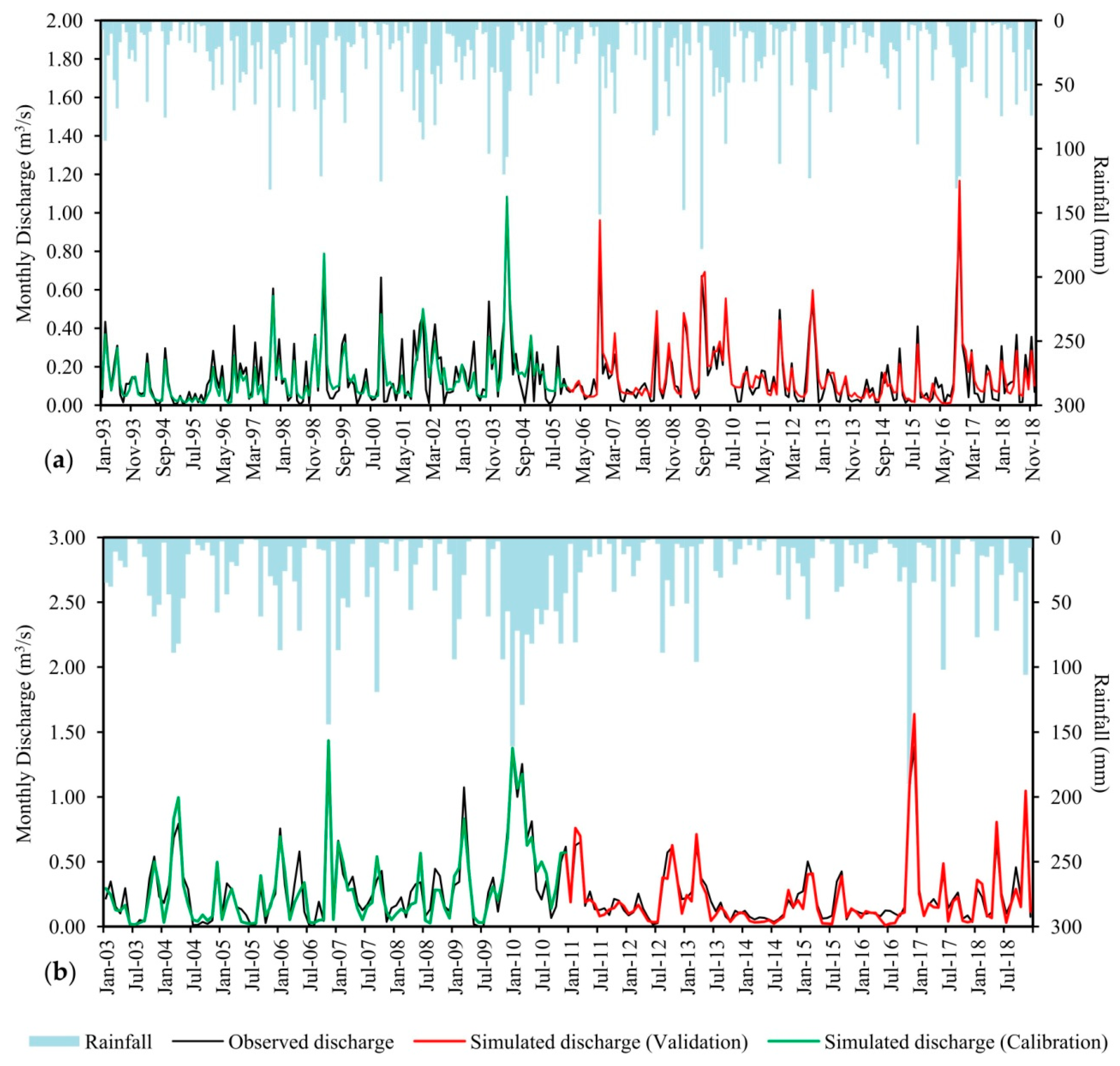
Calibration and Validation

SWAT-CUP software was used for the calibration and validation of the SWAT model. In the calibration phase, a series of warm-up years was used for the Upper Mula basin (1987–1992) and the ephemeral Algeciras stream (1996–2002). For the Upper Mula basin, the information related to the period from 1993–2005 was used in the calibration of the model and that corresponding to the years from 2006–2018 in the validation; for the ephemeral Algeciras stream basin, the period from 2003–2010 was used for the calibration and the 2011–2018 series was used for the validation phase. The method used was the SUFI-2 algorithm (Sequential Uncertainty Fitting) since it requires a smaller number of interactions and a moderate processing time to provide the best result [26]. For the calibration stage, a sensitivity analysis was carried out in order to detect the most influential parameters in the model selected, according to the recommendation of various researchers [19,26,27].

The results were evaluated using six statistical methods, as recommended by Moriasi et al. (2007): (1) Nash–Sutcliffe efficiency (NS) (Equation (3)), (2) percent bias (PBIAS) (Equation (4)), (3) aggregation index (d) (Equation (5)), (4) coefficient of determination (R2) (Equation (6)), (5) root mean square error (RMSE) (Equation (7)), and (6) standard deviation ratio (RSR) (Equation (8)):

$$NS=1-\left[\frac{{{\displaystyle \sum }}_{i=1}^n{(Y_i^{obs}-Y_i^{sim})}^2}{{{\displaystyle \sum }}_{i=1}^n{(Y_i^{obs}-Y_{obs}^{mean})}^2}\right]$$

(3)

$$PBIAS (\%)=\left[\frac{{{\displaystyle \sum }}_{i=1}^n(Y_i^{obs}-Y_i^{sim})·\left(100\right)}{{{\displaystyle \sum }}_{i=1}^n(Y_i^{obs})}\right]$$

(4)

$$d=1-\frac{{{\displaystyle \sum }}_{i=1}^n{(Y_i^{obs}-Y_i^{sim})}^2}{{{\displaystyle \sum }}_{i=1}^n(Y_i^{sim}-\overline{Y_i^{sim}})+Y_i^{obs}-\overline{Y_i^{obs}}{)}^2}$$

(5)

$$R^2=\frac{{\left({{\displaystyle \sum }}_{i=1}^n(Y_i^{obs}-Y_{obs}^{mean})\left(Y_i^{sim}-Y_{sim}^{mean}\right)\right)}^2}{{{\displaystyle \sum }}_{i=1}^n{\left(Y_i^{obs}-Y_{obs}^{mean}\right)}^2{{\displaystyle \sum }}_{i=1}^n{\left(Y_i^{sim}-Y_{sim}^{mean}\right)}^2}$$

(6)

$$RMSE=\sqrt{\frac{{{\displaystyle \sum }}_{i=1}^n{(Y_i^{obs}-Y_i^{sim})}^2}{n}}$$

(7)

$$RSR=\frac{RMSE}{STDE{V}_{obs}}$$

(8)

where $Y_i^{obs}$ and $Y_i^{sim}$ is the evaluated observation and simulation, respectively; $Y_{obs}^{mean}$ and $Y_{sim}^{mean}$ is the mean of the observed and simulated data evaluated; $STDE{V}_{obs}$ is the standard deviation of the observed data; and $n$ is the number of observations. The degree of fit of the results was defined according to the interpretation established by Moriasi et al. [28].

2.4. Climate Scenarios

For our study, the regional climate model (RCM) of the CORDEX initiative was used, and specifically the highest resolution of 0.11 degrees (EUR-11, ~12.5km) of the EURO-CORDEX model. From the basic variables (precipitation and temperatures) of the EURO-CORDEX initiative, the different climate scenarios used in the model were calculated. The choice of the EURO-CORDEX model was based on the good results obtained in studies carried out for Mediterranean regions having semi-arid conditions, which adequately characterized the periods of drought and the torrential phenomena [29,30] typical of this weather. The IPCC scenarios used were RCP 4.5 and RCP 8.5. The former is a moderate scenario and one that assumes that it is possible to reduce greenhouse gases before the year 2050 (+1.5 °C). The RCP 8.5 scenario considers that there will be no change and that greenhouse gases will continue to be emitted uninterrupted throughout the 21st century [3], leading to an increase in the average annual global temperature of 3 °C. Because each climate scenario is subject to the uncertainties inherent to any projection derived from the climate, it is proposed to evaluate the impact taking into consideration a set of climate projections as wide and varied as possible in order to collect a large part of the variability of the climatic hypotheses and reflect the uncertainty (

Table 3. Regional projections obtained with different couplings of global models (GCMs) and regional models (RCMs) of the EURO-CORDEX initiative with a resolution of 0.11°.

GCM	RCM	Institution
CNRM-CM5_r1i1p1	CCLM4-8-17_v1	CLMcom
CNRM-CM5_r1i1p1	ALADIN53_v1	CNRM
CNRM-CM5_r1i1p1	RCA4_v1	SMHI
EC-EARTH_r12i1p1	CCLM4-8-17_v1	CLMcom
EC-EARTH_r12i1p1	RCA4_v1	SMHI
EC-EARTH_r1i1p1	RACMO22E_v1	KNMI
EC-EARTH_r3i1p1	HIRHAM5_v1	DMI
CM5A-MR_r1i1p1	WRF331F_v1	IPSL-INERIS
CM5A-MR_r1i1p1	RCA4_v1	SMHI
HadGEM2-ES_r1i1p1	CCLM4-8-17_v1	CLMcom
HadGEM2-ES_r1i1p1	RACMO22E_v1	KNMI
HadGEM2-ES_r1i1p1	RCA4_v1	SMHI
MPI-ESM-LR_r1i1p1	CCLM4-8-17_v1	CLMcom
MPI-ESM-LR_r1i1p1	RCA4_v1	SMHI
MPI-ESM-LR_r1i1p1	REMO2009	MPI
NorESM1-M	HIRHAM5_v1	DM

). Finally, those projections whose fit was closer to the data of the reference period of each study station were chosen using the normalized root mean square deviation (NRMSD) (Equation (9)), the correlation coefficient (R) (Equation (10)), skill score (SC) (Equation (11)), and rating metrics (RM) (Equation (12)), and once these projections had been selected, their corresponding bias corrections were carried out as follows:

$$NRMSE=\frac{{\left[\frac{1}{\mathrm{N}}{{\displaystyle \sum }}_{i=1}^n{(Y_i^{obs}-Y_i^{sim})}^2\right]}^{1/2}}{Y_{max}-Y_{min}}$$

(9)

$$\mathrm{r}=\frac{\left({{\displaystyle \sum }}_{i=1}^n(Y_i^{obs}-Y_{obs}^{mean})\left(Y_i^{sim}-Y_{sim}^{mean}\right)\right)}{{{\displaystyle \sum }}_{i=1}^n{\left(Y_i^{obs}-Y_{obs}^{mean}\right)}^2{{\displaystyle \sum }}_{i=1}^n{\left(Y_i^{sim}-Y_{sim}^{mean}\right)}^2}$$

(10)

$$SC={{\displaystyle \sum }}_{i=1}^{n}min\left(f_{obs},f_{sim}\right)$$

(11)

$$RM=1-\frac{1}{nm}{{\displaystyle \sum }}_{i=1}^{n}ran{k}_i$$

(12)

where $Y_{max}$ and $Y_{min}$ are the i-th maximum and minimum value observed and simulated in the gridded times series of the climate variables, $N$ is the number of data points in each time series, $f_{obs},f_{sim}$ are the frequencies in the given bin from the observed and model simulated values, and $m$ is the number of metrics.

Statistical Bias Correction Method

Climate projections often exhibit significant biases derived from systematic model errors, and it is advisable to apply different methods to minimize the discrepancy between the observed values of climate variables and the simulated values [31,32,33].

The methods used here for bias correction of the precipitation were Linear Scaling (LS) (Equation (13)), Local Intensity Scaling (LOCI) (Equations (15) and (16)), Power Transformation (PT) (Equations (17)–(19)), Distribution Mapping (DM) (Equations (20) and (21)), Empirical Quantile Mapping (EQM) (Equation (24)), and for temperature, the LS method (Equation (14)), Variance Scaling (VARI) (Equations (26)–(28)), DM (Equations (22) and (23)), and EQM (Equation (25)):

$$\left(LS\right) P_{hst,m,d}^{cor}=P_{raw,m,d}*\frac{\mu \left(P_{obs,m}\right)}{\mu \left(P_{raw,m}\right)}$$

(13)

$$\left(LS\right)T_{raw,m,d}^{cor}=T_{raw,m,d}+\mu \left(T_{obs,m}\right)-\mu \left(T_{obs,m}\right)$$

(14)

$$\left(LOCI\right)S_m=\frac{\mu (P_{obs,m,d}|P_{obs,m,d}\rangle 0}{\mu (P_{raw,m,d}|P_{raw,m,d}\rangle P_{thres,m}}$$

(15)

$$\left(LOCI\right)P_{raw,m,d}^{cor}=\{\begin{array}{c}{P}_{raw,m,d}\times S_m{P}_{raw,m,d}>P_{thres,m}\\ 0 P_{raw,m,d}<P_{thres,m}\end{array}$$

(16)

$$\left(PT\right)f\left(b_m\right)=\frac{\sigma \left(P_{obs,m}\right)}{\mu \left(P_{obs,m}\right)}-\frac{\sigma \left(P_{LOCI,m}^{b_m}\right)}{\mu \left(P_{LOCI,m}^{b_m}\right)}$$

(17)

$$\left(PT\right)S_m=\frac{\mu \left(P_{obs,m}\right)}{\mu \left(P_{LOCI,raw,m,d}^{b_m}\right)}$$

(18)

$$\left(PT\right)P_{raw,m,d}^{cor}=S_m\times P_{LOCI,raw,m,d}^{b_m}$$

(19)

$$\left(DM\right)f_{\gamma }\left(x|\mu ,\beta \right)=x^{\alpha -1}\times \frac{1}{{\beta }^{\alpha }\times \Gamma \left(\alpha \right)}\times e^{\frac{-x}{\beta }}; x \ge 0;\alpha ,\beta >0$$

(20)

$$\left(DM\right)P_{raw,m,d}^{cor}=F_{\gamma }^{-1}(F_{\gamma }\left(P_{LOCI,raw,d}|\alpha P_{LOCI,raw,},\alpha P_{LOCI,raw,}\right)$$

(21)

$$\left(DM\right)f_{\gamma }\left(x|\mu ,{\sigma }^2\right)=\frac{1}{\sigma \times \sqrt{2\pi }}\times e^{\frac{-{\left(x-\mu \right)}^2}{2{\sigma }^2}}; x ϵ R$$

(22)

$$\left(DM\right)T_{raw,m,d}^{cor}=F_N^{-1}(F_N\left(T_{raw,m,d}|{\mu }_{raw,m},{\sigma }_{raw,m}^2\right)|{\mu }_{obs,m},{\sigma }_{obs,m}^2)$$

(23)

$$\left(EQM\right)P_{raw,m,d}^{cor}=ecd{f}_{obs,m}^{-1}\left(ecd{f}_{raw,m}\left(P_{raw,m,d}\right)\right)$$

(24)

$$\left(EQM\right)T_{raw,m,d}^{cor}=ecd{f}_{obs,m}^{-1}\left(ecd{f}_{raw,m}\left(T_{raw,m,d}\right)\right)$$

(25)

$$\left(VARI\right)T_{raw,m,d}=T_{raw,m,d}-\mu \left(T_{raw,m,d}\right)$$

(26)

$$\left(VARI\right){\sigma }_{raw,m,d}=T_{raw,m,d}\times \frac{{\sigma }_m\left(T_{obs,m}\right)}{{\sigma }_m\left(T_{raw,m}\right)}$$

(27)

$$\left(VARI\right)T_{raw,m,d}^{cor}={\sigma }_{raw,m,d}+\mu \left(T_{raw,m,}\right)$$

(28)

where $P_{hst,m,d}^{cor}$ is the corrected precipitationon the $d$-th day of the$m$-th month; $T_{raw,m,d}^{cor}$ is the corrected temperature on the $d$-th day of the $m$-th month; $P_{raw,m,d}$ is the precipitationfrom original RCM outputs during the relevant period; $T_{raw,m,d}$ is the temperature from the original RCM outputs during the relevant period; $P_{obs,m}$ is the mean value of the observed precipitation at a given $m$-th month; $T_{obs,m}$ is the mean value of the observed temperature at a given $m$-th month;$\mu$ is the mean value; $S_m$ is the scaling factor; $P_{thres,m}$ is the rainfall intensity threshold for each $m$-th month; $\sigma$ is the standard deviation value; $b_m$ is the exponent for the $m$-th month; $P_{LOCI,m}$ is the LOCI corrected precipitation in the $m$-th month; $\Gamma (.)$ is the Gamma function; $\alpha$ and $\beta$ are the form and scale parameters, respectively; $F_{\gamma }$ and $F_{\gamma }^{-1}$ represent the Gamma cumulative distribution functions ($ecdfs$); $F_N$ and $F_N^{-1}$ represent the Gamma cumulative distribution functions ($ecdfs$) for the temperature; and $ecd{f}^{-1}$ is the inverse of the Gamma cumulative distribution function for the $ecdfs$.

For this, the reference period from 1988–2005 was used for the stations of the Upper Mula basin and the period from 1996–2005 was used for the stations of the Algeciras basin; finally, those that showed a better goodness of fit were selected, based on the statistics in Equations (3) and (4), for inclusion in the SWAT model configuration.

3. Results and Discussion

3.1. Sensitivity Analysis

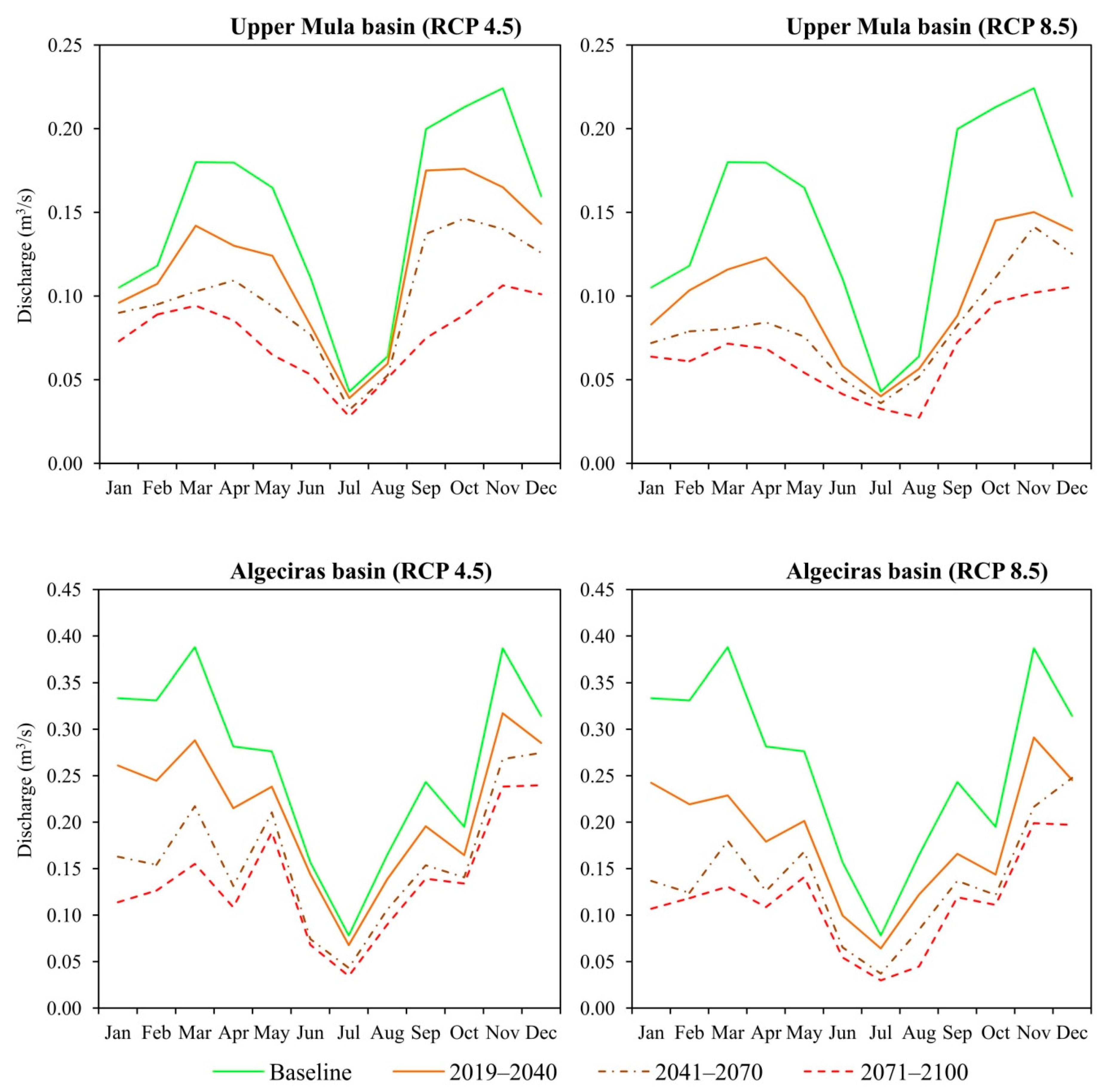
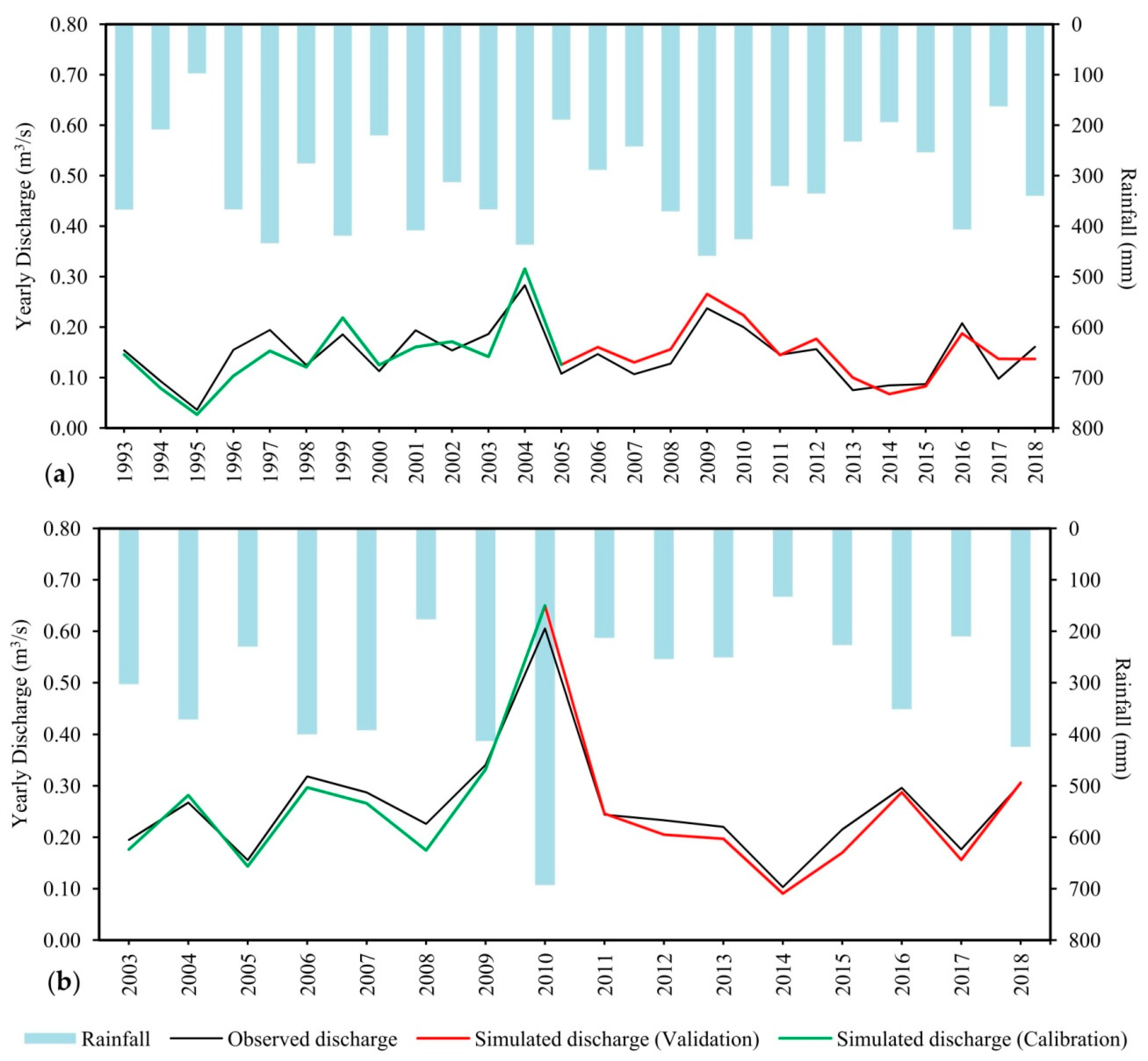
In the sensitivity analysis, the measurement data corresponding to the period from 1993–2005 for the Upper Mula stream and to the period from 2003–2010 for the ephemeral Algeciras stream were used, with a series of warm-up periods of 6 (1987–1992) and 7 years (1996–2002), respectively.

The parameters used to perform the sensitivity analysis were chosen following the methodology of Martínez-Salvador and Conesa-García [27], where 29 parameters were tested for the analysis of the flow under environmental conditions similar to those of the study basins of the present work. The simulations carried out for the Algeciras and Upper Mula basins showed differences in the behavior of the sensitivity between them, conditioned by the climatic and geological differences between the two basins.

Table 4. Ranking of the most influential parameters in the flow simulation.

Parameter	Upper Mula Basin				Algeciras Basin
	Rank	p-Value	t-Stat	Fitted Value	Rank	p-Value	t-Stat	Fitted Value
ALPHA_BF.gw	16	0.41	−0.83	0.79	12	0.35	−0.96	0.40
ALPHA_BNK.rte	5	0.03	2.31	0.78	21	0.65	−0.46	0.83
BIOMIX.mgt	11	0.28	−1.12	0.53	9	0.25	−1.19	1.15
CH_K2.rte	3	0.00	4.79	1.62	2	0.05	−2.04	1.02
CH_N2.rte	10	0.25	1.18	−0.07	3	0.06	−2.04	−15.99
CN2.mgt	23	0.72	0.37	0.13	22	0.68	−0.41	−0.08
DEEPST.gw	15	0.41	−0.85	38,612.08	20	0.63	−0.49	21,324.44
ESCO.hru	1	0.00	−13.92	0.65	16	0.43	0.81	0.82
FFCB.bsn	27	0.96	0.05	0.55	24	0.72	−0.36	1.65
GW_DELAY.gw	26	0.91	0.11	514.51	14	0.39	0.88	388.13
GW_SPYLD.gw	14	0.36	0.94	0.14	13	0.36	0.93	0.34
GWQMN.gw	12	0.30	−1.06	0.27	23	0.69	0.40	0.83
HRU_SLP.hru	2	0.00	−15.81	−0.01	7	0.14	−1.54	0.07
OV_N.hru	17	0.44	0.79	−0.03	4	0.06	−1.98	−0.04
PLAPS.sub	13	0.34	−0.97	206.64	6	0.12	1.62	153.81
RCHRG_DP.gw	29	0.99	0.01	−0.39	25	0.76	−0.31	0.02
REVAPMN.gw	28	0.99	−0.02	−186.98	26	0.79	−0.27	−107.76
SFTMP.bsn	21	0.63	0.49	3.92	15	0.40	−0.86	−5.06
SHALLST.gw	20	0.54	−0.62	29,527.58	10	0.29	−1.09	48,833.96
SLSUBBSN.hru	22	0.67	−0.43	0.06	5	0.09	−1.76	0.03
SMFMX.bsn	19	0.51	0.67	10.33	11	0.29	1.08	−2.17
SMTMP.bsn	8	0.20	−1.34	31.03	17	0.44	−0.79	14.74
SOL_BD(..).sol	4	0.00	−3.71	0.19	28	0.93	−0.09	0.11
SOL_CRK.sol	6	0.12	−1.64	0.04	19	0.61	−0.52	0.39
SOL_K(..).sol	25	0.91	−0.12	0.39	1	0.00	3.86	2.01
SURLAG.bsn	24	0.84	0.20	16.23	27	0.86	−0.18	2.33
TIMP.bsn	9	0.25	−1.20	0.45	29	1.00	0.00	0.76
TLAPS.sub	18	0.48	0.72	2.99	8	0.23	1.25	11.70
TRNSRCH.bsn	7	0.17	1.42	7.19	18	0.47	−0.74	8.27

summarizes these values for both basins.

In the Upper Mula basin, this analysis verified that the most sensitive parameters in the prediction of the flow were the compensation factor for evaporation in the soil (ESCO), the average slope steepness (HRU_SLP), the hydraulic conductivity of the main channel (CH_K2), the humid apparent density of the soil (SOL_BD), and the factor of the base flow in the bank storage (ALPHA_BNK). It can be highlighted how the evaporation, lateral flow, and base flow storage regulate the hydrological regime of the Upper Mula stream, similar to the results in other studies [34,35].

The high sensitivity of the ESCO parameter is very important as it is related to the high evapotranspiration in these semi-arid regions of the Mediterranean basin [36,37] and, in this case, it represents the forest that accounts for about 39% of the land use within the Upper Mula basin, and in the case the Algeciras basin, for about 27%.

In the case of the Algeciras basin, the most sensitive parameters were the saturated hydraulic conductivity (SOL_K), the hydraulic conductivity of the main channel (CH_K2), the Manning roughness coefficient for the main channel (CH_N2), the value “Manning’s n” for overland flow (OV_N), and the mean slope length (SLSUBBSN) (Table 4). Because a large part of the basin is dominated by clay materials, forming a large badlands complex, the high sensitivity of these parameters indicates the importance of lateral flow within the kinematic storage model [38,39].

The values of the parameters estimated by SWAT were within the expected ranges and described the hydrological processes of the Upper Mula stream and the ephemeral Algeciras stream based on the observations of precipitation and flow. The final calibrated obtained values helped to identify the differences between the two basins. The hydraulic conductivity of the main channel constitutes a parameter of great importance since it describes the mobility of sub-surface or underground water and is common to both basins due to the importance of the aquifer system and its groundwater in the hydrology of these basins. The values of the CH_K2 parameter were 1.62 mm/h for the Upper Mula stream and 1.02 mm/h for the ephemeral Algeciras stream, which implies the presence of flow losses within the basins [40].

3.2. Hydrology

The simulated flows in the calibration and validation periods for both basins were able to optimally reproduce the flows observed on a monthly and annual scale (

Table 5. Evaluation of the performance of the SWAT model in the calibration and validation of the monthly and yearly runoff simulations.

Statistic	Upper Mula Basin				Algeciras Basin
	Calibration		Validation		Calibration		Validation
	Monthly	Yearly	Monthly	Yearly	Monthly	Yearly	Monthly	Yearly
d	0.94	0.94	0.97	0.95	0.97	0.99	0.98	0.97
R2	0.79	0.82	0.88	0.85	0.88	0.99	0.94	0.96
NS	0.79	0.76	0.86	0.78	0.88	0.95	0.91	0.86
RSR	0.46	0.47	0.38	0.45	0.35	0.20	0.29	0.35
PBIAS %	−4.50	−4.70	7.40	7.40	−2.50	−3.00	−7.10	−7.50
RMSE	0.07	0.03	0.06	0.02	0.10	0.03	0.07	0.02

).

The values of NS, RSR, and PBIAS are very good, according to the criteria of Moriasi et al. [28], for all the calibration and validation phases of the Upper Mula stream and the ephemeral Algeciras stream.

The NS values are above 0.75, with an improvement in the validation phases, with the exception of the ephemeral Algeciras stream. The PBIAS based on monthly and annual values shows a slight underestimation of the flow in the calibration and validation, except in the validation phase for the Upper Mula stream, when it overestimates the observed flows by 7.40%. The magnitudes of this value are low, indicating a very good fit.

The RSR, NS, d, and R² values estimated in the validation period of the monthly and annual flow rates represent an improvement in the quality of fit compared to the calibration values. Although this does not occur frequently, some authors have also documented a statistical improvement in the validation phase [15,27]. This improvement indicates that the simulated results have lower uncertainty.

Figure 3a,b show the simulated monthly hydrographs for the Upper Mula stream and the ephemeral Algeciras stream. The data simulated by the model fit very closely, although it is observable how the flow tends to be overestimated in dry periods. This overestimation may indicate that the model does not fully capture the dynamics of the groundwater components [41,42] or is not adequately simulating the evapotranspiration capacity of the vegetation [43], and therefore that the soil and base flow parameters did not vary enough to guarantee a better representation of the surface runoff processes.

In addition, a slight overestimation of the maximum monthly flow can also be observed for both channels, which may be because the different porosities and hydraulic conductivities present in these basins led the SWAT model to interpret the existence of less water infiltration towards the subsoil.

These results indicate that SWAT had some difficulty in simulating low flow rates, such as those found in Mediterranean climates with semi-arid characteristics. Zhang et al. [44] pointed out that this inaccuracy of the model during dry periods can also be associated with the choice of the objective function (NS) used to calibrate the model, which tends to give more weight to torrential events, and therefore, these are fitted better in the wettest months where the flow is overestimated due to excess precipitation, and this is not distributed as flow throughout the next month.

On an annual scale (Figure 4a,b) we can observe this tendency of the model to give an underestimation in the driest years and a slight overestimation in the wettest years.

In general, the results of the model for both basins show an underestimation of the average flow in the calibration and validation periods, with the exception of the validation stage for the Upper Mula basin, where this trend is reversed.

In one respect, these difficulties of the model to reproduce the flows in times of drought or rainfall decrease are due to the inability of SWAT to simulate the interaction between the surface runoff and the underground flow, since a complex system of aquifers extends over both basins.

In various studies, comparison of the hydrographs showed these limitations of the SWAT model, especially in terms of the tendency to underestimate the flow during the driest years [45,46]. Therefore, the SWAT simulations should be improved to achieve a better prediction of the flow in periods that contain episodes of drought.

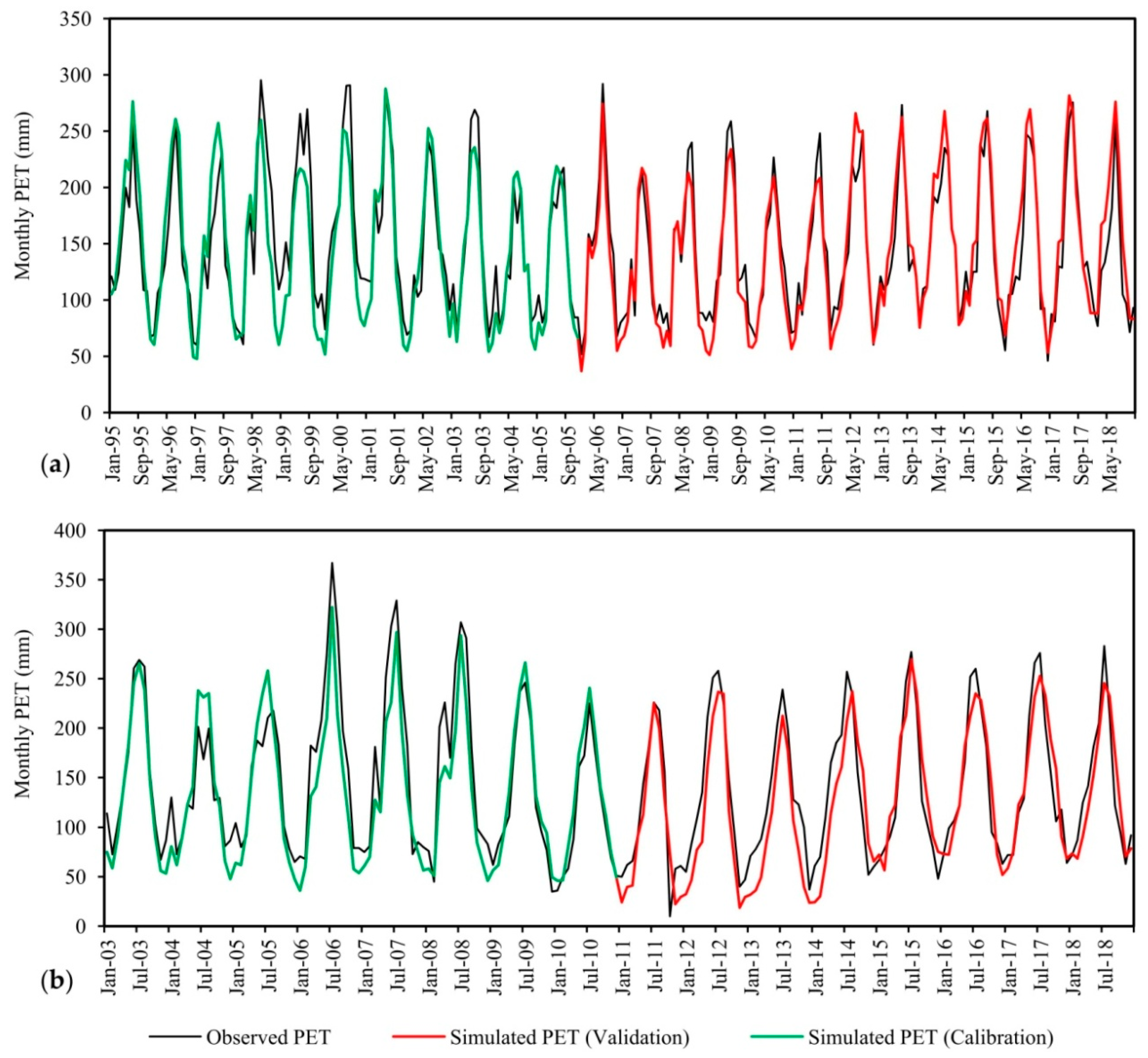
3.3. Evapotranspiration

The observed values of the monthly and annual evapotranspiration for the Upper Mula and Algeciras basins (

Table 6. Evaluation of the performance of the SWAT model in the calibration and validation of the monthly and yearly PET simulations.

Statistic	Upper Mula Basin				Algeciras Basin
	Calibration		Validation		Calibration		Validation
	Monthly	Yearly	Monthly	Yearly	Monthly	Yearly	Monthly	Yearly
d	0.95	0.93	0.97	0.96	0.95	0.94	0.95	0.93
R2	0.82	0.78	0.89	0.87	0.86	0.92	0.85	0.86
NS	0.79	0.76	0.87	0.79	0.78	0.83	0.82	0.85
RSR	0.46	0.47	0.36	0.44	0.41	0.39	0.42	0.47
PBIAS %	−4.00	−1.50	0.70	0.70	−8.10	−1.60	−8.20	−0.50
RMSE	28.12	95.09	16.93	47.27	31.29	112.35	29.66	66.70

) and those simulated in the sub-basins where their respective reservoirs are located showed very high statistical goodness-of-fit according to the criteria of Moriasi et al. [28].

The NS values are above 0.75 in the calibration stage, being improved in the validation stage for both basins. The PBIAS values also show an improvement in the validation phase, with monthly and annual values close to 0 (0.70%) for the Upper Mula basin.

The annual RMSE for both basins improves substantially in the validation stage and therefore, together with RSR values lower than 0.50, it shows the low uncertainty of the simulated PET values.

Figure 5 shows how the simulated PET values fit the variability of the observed evaporation values recorded in the La Cierva and Algeciras reservoirs, with the exception of the extreme values (maximum and minimum), for which the SWAT tends to underestimate PET, repeating this trend throughout the series.

The peaks of PET are concentrated from May to August, with the maximum values being between July and August, something quite expected as these are data for a Mediterranean climate in a semi-arid region of southeastern Spain. The maximum values recorded in the Upper Mula and Algeciras basins were 292 and 360 mm, respectively, both in July 2006, and the lowest values occurred in December 2016 (46.1 mm—Mula) and in October 2011 (10.1 mm—Algeciras). In the four cases, SWAT slightly underestimated the values. Similar results were reported by Rao et al. [47] and Samadi [25] for climatic conditions similar to those of our study area.

The PET calculation correctly reproduces the meteorological data from the La Cierva and Algeciras stations, ensuring low uncertainty in the simulation of these processes, essential for the continuous simulation and under different climate change scenarios.

3.4. Application of Bias Correction Methods for Hydrological Modeling

The bias correction was performed for those historical RCMs that fitted better the data recorded for the variables at the different stations of the study area. As can be seen in

Table A1. Accuracy assessment of RCMs at stations of the Upper Mula basin.

RCMs	Upper Mula Basin
	Prec			Tmax			Tmin
	NRMSE	r	SS	NRMSE	r	SS	NRMSE	r	SS
CNRM-CCLM4-8-17	0.233	0.770	0.965	0.124	1.000	0.995	0.155	1.000	0.986
CNRM-ALADIN53	0.828	−0.220	0.769	0.098	1.000	0.997	0.482	1.000	0.819
CNRM-RCA4	0.466	0.750	0.909	0.100	0.990	0.997	0.310	1.000	0.931
ICHEC-CCLM4-8-17	0.310	0.820	0.923	0.119	1.000	0.996	0.170	1.000	0.982
ICHEC-HIRHAM5	0.328	0.750	0.939	0.182	1.000	0.989	0.132	0.990	0.989
ICHEC-RACMO22E	0.560	0.540	0.873	0.158	1.000	0.992	0.356	1.000	0.906
ICHEC-RCA4	0.293	0.660	0.949	0.113	1.000	0.996	0.357	1.000	0.904
IPSL-WRF331F	1.690	−0.890	0.329	0.188	1.000	0.988	0.139	0.990	0.988
IPSL-RCA4	0.569	−0.130	0.674	0.066	1.000	0.999	0.267	1.000	0.952
MOHC-CCLM4-8-17	0.284	0.860	0.938	0.119	1.000	0.996	0.132	1.000	0.990
MOHC-RACMO22E	0.431	0.690	0.918	0.086	1.000	0.998	0.269	1.000	0.953
MOHC-RCA4	0.621	0.590	0.858	0.100	1.000	0.997	0.256	1.000	0.956
MPI-CCLM4-8-17	0.284	0.620	0.944	0.083	1.000	0.998	0.098	1.000	0.995
MPI-REMO2009	0.362	0.730	0.938	0.049	1.000	0.999	0.081	1.000	0.996
MPI-RCA4	0.560	0.440	0.873	0.064	0.990	0.999	0.249	1.000	0.958
NCC-HIRHAM5	0.397	0.530	0.894	0.121	0.990	0.995	0.070	0.990	0.997

,

Table A2. Accuracy assessment of RCMs at stations of the Algeciras basin.

RCMs	Algeciras Basin
	Prec				Tmax			Tmin
	NRMSE	r	SS	NRMSE		r	SS	NRMSE	r	SS
CNRM-CCLM4-8-17	0.204	0.810	0.960	0.164		0.990	0.991	0.098	0.990	0.994
CNRM-ALADIN53	0.912	−0.200	0.690	0.115		1.000	0.996	0.255	1.000	0.940
CNRM-RCA4	0.292	0.700	0.936	0.146		0.980	0.993	0.079	0.990	0.995
ICHEC-CCLM4-8-17	0.350	0.540	0.872	0.166		0.990	0.990	0.067	0.990	0.997
ICHEC-HIRHAM5	0.482	0.760	0.876	0.206		0.990	0.985	0.128	0.990	0.989
ICHEC-RACMO22E	0.737	0.480	0.763	0.225		0.990	0.981	0.156	0.990	0.979
ICHEC-RCA4	0.365	0.520	0.885	0.170		0.990	0.990	0.128	1.000	0.986
IPSL-WRF331F	0.987	−0.790	0.305	0.202		0.990	0.985	0.138	0.990	0.988
IPSL-RCA4	0.584	0.450	0.472	0.047		0.990	0.999	0.053	1.000	0.998
MOHC-CCLM4-8-17	0.190	0.880	0.964	0.109		1.000	0.996	0.146	0.990	0.987
MOHC-RACMO22E	0.650	0.480	0.814	0.121		1.000	0.995	0.087	1.000	0.994
MOHC-RCA4	0.270	0.760	0.953	0.086		0.990	0.998	0.039	1.000	0.999
MPI-CCLM4-8-17	0.328	0.480	0.917	0.113		1.000	0.996	0.134	1.000	0.989
MPI-REMO2009	0.431	0.520	0.879	0.020		1.000	1.000	0.145	1.000	0.987
MPI-RCA4	0.365	0.620	0.911	0.102		1.000	0.997	0.030	1.000	0.999
NCC-HIRHAM5	0.307	0.630	0.923	0.151		0.990	0.992	0.217	0.980	0.972

and

Table A3. Rating metric of RCMs for the Upper Mula and Algeciras basin.

RCMs	Upper Mula Basin			Algeciras Basin
	Prec Rank	Tmax Rank	Tmin Rank	RM	Prec Rank	Tmax Rank	Tmin Rank	RM
CNRM-CCLM4-8-17	2	11	7	5	1	13	7	4
CNRM-ALADIN53	14	7	16	14	14	6	16	14
CNRM-RCA4	4	9	5	4	9	8	13	12
ICHEC-CCLM4-8-17	11	12	4	10	7	11	8	9
ICHEC-HIRHAM5	10	15	8	12	4	15	5	6
ICHEC-RACMO22E	13	16	14	16	11	14	14	16
ICHEC-RCA4	8	13	13	13	2	9	15	10
IPSL-WRF331F	16	14	10	15	16	16	6	15
IPSL-RCA4	15	2	3	6	15	2	12	11
MOHC-CCLM4-8-17	1	5	11	3	6	10	4	3
MOHC-RACMO22E	12	8	6	9	8	5	11	7
MOHC-RCA4	3	3	2	1	13	7	10	13
MPI-CCLM4-8-17	6	6	9	7	3	4	3	2
MPI-REMO2009	9	1	12	8	5	1	2	1
MPI-RCA4	7	4	1	2	12	3	9	8
NCC-HIRHAM5	5	10	15	11	10	12	1	5

in Appendix A, the RCMs selected were those that had a priori the best RM values without applying any statistical correction method for both catchments.

The models selected to apply the different bias correction techniques were the following: the MPI-REMO2009 model was selected for the Upper Mula basin and the MOHC-RCA4 model for the Algeciras basin.

The bias corrections applied to each of the data sources improved them considerably compared to the reference period.

Table 7. Performance of RCM outputs at stations of the Upper Mula basin.

Methods	Upper Mula Basin
	La Cierva						Pinar Hermoso		Lorca Coy
	Prec		Tmax		Tmin		Prec		Prec
	NS	PBIAS (%)	NS	PBIAS (%)	NS	PBIAS (%)	NS	PBIAS (%)	NS	PBIAS (%)
RAW	0.02	15.71	0.89	−4.05	0.90	5.77	−0.09	17.98	0.14	20.41
LS	0.89	−3.59	0.98	1.85	0.92	7.89	0.70	6.65	0.82	−2.88
LOCI	0.94	1.00	-	-	-	-	0.87	−4.25	0.91	0.79
PT	0.85	−2.88	-	-	-	-	0.79	5.79	0.74	−7.85
DM	0.61	5.86	0.96	2.69	0.93	4.74	0.61	10.47	0.61	5.74
EQM	0.79	−3.38	0.96	2.10	0.95	−2.24	0.84	6.52	0.80	8.67
VARI	-	-	0.99	0.10	0.99	0.58	-	-	-	-

and

Table 8. Performance of RCM outputs at stations of the Algeciras basin.

Methods	Algeciras Basin
	Los Quemados						Gebas
	Prec		Tmax		Tmin		Prec
	NS	PBIAS (%)	NS	PBIAS (%)	NS	PBIAS (%)	NS	PBIAS (%)
RAW	0.24	10.83	1.00	0.29	0.99	0.43	−0.02	−19.94
LS	0.80	−3.77	0.98	−0.94	0.99	−0.96	0.84	3.25
LOCI	0.91	2.64	-	-	-	-	0.93	2.21
PT	0.79	−9.44	-	-	-	-	0.80	−5.78
DM	0.71	9.75	0.97	−0.16	0.96	1.28	0.69	9.96
EQM	0.70	−8.69	0.98	−0.78	0.99	2.19	0.82	5.88
VARI	-	-	1.00	0.27	1.00	0.05	-	-

show the NS and PBIAS values for the series of precipitation, maximum temperature, and minimum temperature of the stations of the Upper Mula basin (La Cierva, Pinar Hermoso, and Lorca Coy) and the Algeciras basin (Los Quemados and Gebas) after applying the statistical correction from the LS, LOCI, PT, DM, EQM, and VARI methods.

All the applied methods substantially improved the fits between the observed series and the historical projected series, although with some differences. For the maximum and minimum temperature, there were no significant differences among the different correction methods. The method that provided the best correction for the La Cierva and Los Quemados stations was the VARI. On the other hand, for the series of precipitation, relative humidity, and wind speed, important differences were obtained. The best correction method for these series was the LOCI, which provided NS values above 0.90 and PBIAS close to 0, followed by the LS model. Both models produce better results in time series based on the precipitation means than those based on the quantile-based methods, such as the EQM method. The LOCI method provides a good estimate of the mean, the median, the probability of wet days, and the intensity of wet days. On the other hand, there is an overestimation in the standard deviation that does not occur with the PT method, these results being consistent with those obtained by other researchers in other regions [48,49]. The DM method was the one that provided the worst fit, perhaps due to the fact that it is more appropriate for more humid regions such as northern Europe [50].

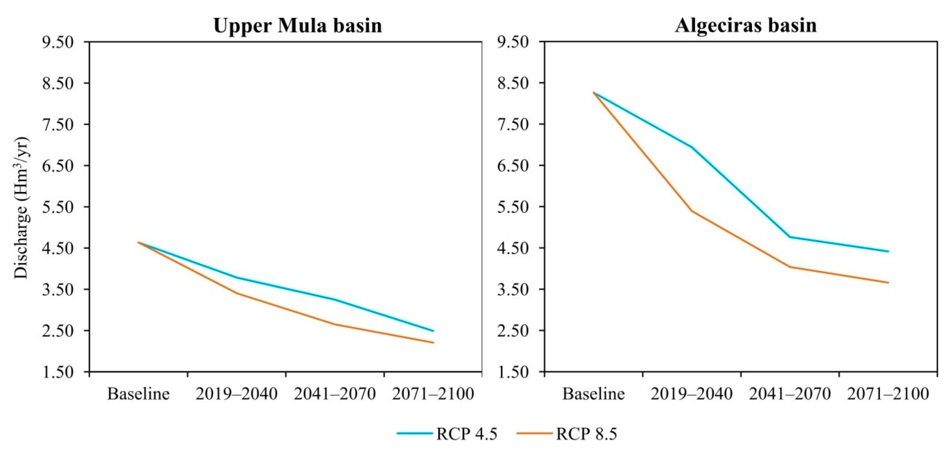
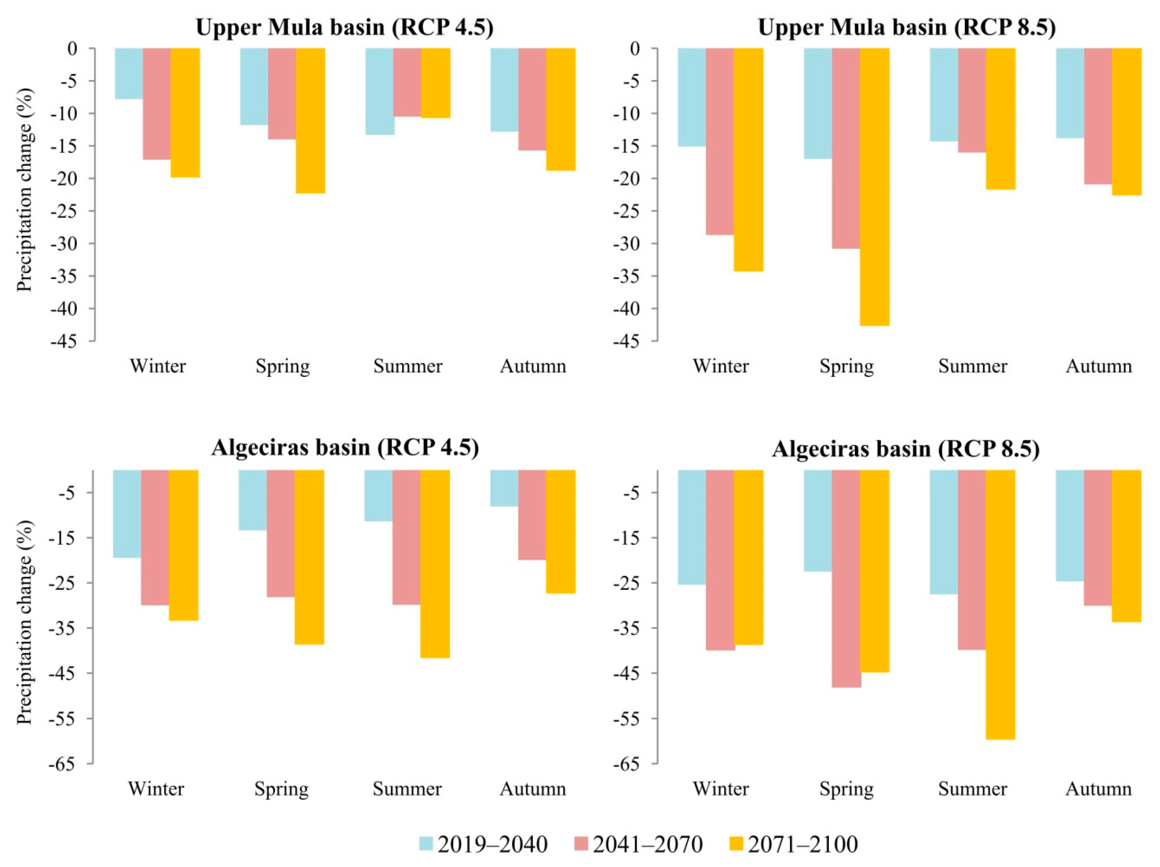
3.5. Changes in Climate Variables under RCP Scenarios

Table 9. Average values of the flow (m³/s), precipitation (mm), temperature (°C), PET (mm), and RET (mm) in the Upper Mula basin; within the parentheses are the percentage changes with respect to the baseline period.

Variable	Baseline (1993–2018)	Period (2019–2040)		Period (2041–2070)		Period (2071–2100)
		RCP 4.5	RCP 8.5	RCP 4.5	RCP 8.5	RCP 4.5	RCP 8.5
Prec (mm)	351.67	306.6 (−12.8%)	301.5 (−14.3%)	297.9 (−15.3%)	276.2 (−21.8%)	290.1 (−17.5%)	253.5 (−27.9%)
T (°C)	17.68	17.9 (1.45%)	18 (1.8%)	18.3 (3.4%)	18.9 (6.7%)	18.7 (5.8%)	20.2 (13.9%)
Q (m3/s)	0.147	0.120 (−18.4%)	0.108 (−26.2%)	0.103 (−29.70%)	0.084 (−42.8%)	0.079 (−46.3%)	0.07 (−52.4%)
PET (mm)	1777.57	1783.2 (0.32%)	1793.5 (0.9%)	1831.9 (3%)	1880.2 (5.8%)	1853.2 (4.3%)	2027.1 (14.1%)
RET (mm)	280.83	279.2 (−0.6%)	298.1 (6.2%)	281.1 (0.1%)	256.8 (−8.6%)	273.9 (−2.5%)	233.4 (−16.9%)

and

Table 10. Average values of the flow (m³/s), precipitation (mm), temperature (°C), PET (mm), and RET (mm) in the Algeciras basin; within the parentheses are the percentage changes with respect to the baseline period.

Variable	Baseline (1993–2018)	Period (2019–2040)		Period (2041–2070)		Period (2071–2100)
		RCP 4.5	RCP 8.5	RCP 4.5	RCP 8.5	RCP 4.5	RCP 8.5
Prec (mm)	334.5	295.7 (−11.6%)	268.2 (−19.9%)	239.8 (−28.3%)	200.2 (−40.1%)	230.5 (−31.2%)	187.7 (−43.9%)
T (°C)	16.4	18.1 (10.1%)	18 (10.9%)	18.7 (14.5%)	19.5 (18.8%)	19.5 (19.2%)	21.3 (29.5%)
Q (m3/s)	0.262	0.22 (−16%)	0.171 (−34.8%)	0.151 (−42.4%)	0.128 (−51.2%)	0.14 (−46.6%)	0.116 (−55.8%)
PET (mm)	1690.57	1857 (9.8%)	1910.2 (13%)	1963 (16.1%)	2189.7 (29.5%)	2056.1 (21.6%)	2359.2 (39.5%)
RET (mm)	239.46	235.8 (0.6%)	215 (−10.2%)	227.8 (−4.9%)	205.8 (−14.1%)	210.4 (−12.2%)	198.3 (−17.9%)

show the changes in the variables discharge, precipitation, potential evapotranspiration, and real evapotranspiration (RET) once the biases of the different climate scenarios used in the SWAT model had been corrected. Similar patterns can be observed in both basins, with a generalized reduction in all variables, except T and PET, which experience increases throughout the different future time periods.

The flows in both basins experience a significant decrease in water inputs. According to the projections, for the most extreme scenario (RCP 8.5) in the Upper Mula and Algeciras basins, there would be a decrease in flows of around 42.8% and 51.2%, respectively, for the period from 2041–2070, and this decrease would be more pronounced for the period from 2071–2100 (52.4% and 55.8%, respectively). Precipitation would be around 27.9% and 43.9% lower, respectively, by the end of the 2071–2100 period in the most extreme scenario. Not surprisingly, RET would also suffer a decrease as precipitation decreases. In contrast, PET would undergo a significant increase as a consequence of the increase in the mean temperature in both basins, further intensifying the semi-arid characteristics that characterize them.

Therefore, climate change is expected to have a significant impact on the water inputs of both basins. Figure 6 clearly shows how the water resources tend to decline as we approach the end of the century.

If we evaluate the possible impact of climate change by comparing the future assembly of each period (2019–2040, 2041–2070, and 2071–2100) with the reference one, in the first period under the RCP 4.5 and RCP 8.5 scenarios, the water contributions would be reduced by around 0.85 Hm³/year and 1.23 Hm³/year, respectively, for the Upper Mula basin, and by around 1.32 Hm³/year and 2.87 Hm³/year for the Algeciras basin. In the medium term (2041–2070), the water contributions would continue to decrease, the overall decline being 1.39 Hm³/year for the RCP 4.5 scenario and 1.99 Hm³/year for the RCP 8.5 scenario in the Upper Mula basin and 3.5 Hm³/year (RCP 4.5) and 4.23 Hm³/year (RCP 8.5) for the Algeciras basin. Hence, the models predict that the reductions will be more pronounced for the Algeciras basin. However, according to the most extreme models, these reductions could reach 4.60 Hm³/year (RCP 8.5) for the Algeciras basin and 2.43 Hm³/year (RCP 8.5) for the Upper Mula basin. These results are consistent with other studies in Mediterranean areas with similar environmental characteristics [30,51].

Changes in precipitation explain this important decrease in the flows in both basins, while later changes could be due also to increased infiltration and PET. It is precisely this increase in PET that leads to a reduction in available resources, both superficial (in floods, as the Algeciras is an ephemeral stream) and underground (in the form of recharge to the aquifers present in both basins). An increase in evapotranspiration of between 15% and 39% causes a reduction in the available water resources of between 52% and 56%.

This trend towards a decrease could pose a great challenge for the future management of the water resources in these basins, since currently the generated resources and demands are very similar, around 90% [52]. However, these reductions seem very large if we take into account other studies that have been carried out in this area, such as the CEDEX [53], in which average (RCP 4.5 and 8.5) runoff reductions of 7%, 18%, and 28% for the entire CHS were reported.

These results are based on static characteristics in both basins. Probably, the decrease in precipitation and change to a more severely arid climate will likely result in vegetation changes due to a shortage of water and increased vulnerability to pests and disease, which will have a profound effect on annual evapotranspiration.

Figure 7 shows the monthly flow values for the baseline and for the RCP 4.5 and 8.5 scenarios.

The results of the model show that the flow of the Upper Mula stream and the ephemeral Algeciras stream would decrease in all months of the year, especially in the periods when the flow is generally high in both basins (November to May) during the historical period, reaching monthly flows as low as 0.029 and 0.045 m³/s (July and August) for the period 2071–2100 in the case of the Algeciras basin, and 0.028 and 0.051 m³/s (July and August) in the case of the Mula basin.

All the scenarios analyzed reveal a severe impact of climate change in flows. In addition, days with zero flow in the Upper Mula stream and the ephemeral Algeciras stream are more common, which could have serious environmental consequences.

At the seasonal level (Figure 8), the changes are more palpable, with all the estimated climatic scenarios showing a generalized reduction in flows. In summer, a significant decrease in flow is estimated due to the decrease in precipitation and an increase in evapotranspiration. The present results are consistent with many previous studies under semi-arid climates [29,51].

Figure 9 shows the Stream Drought Index (SDI) applied for all the scenarios analyzed in both basins. The SDI reveal a severe impact of climate change in flows with an increase in the periods of moderate, severe, and extreme drought.

The periods of drought in both basins experience a significant increase compared to the baseline. According to the projections, for the most extreme scenario (RCP 8.5) in the Upper Mula and Algeciras basins, there would be an increase in extreme prolonged drought episodes over time (around 6 years), being more pronounced for the 2075–2100 period. The droughts will tend to become more frequent in any of the contemplated time periods. Short-term droughts (up to 3 years) will be more frequent and intense in the last period of the 21st century. These results are consistent with those obtained by CEDEX [53].

4. Conclusions

The combination of the SWAT hydrological model and the different climate scenarios made it possible to simulate the possible effects of climate change on the flows of the Upper Mula stream and the ephemeral Algeciras stream. For this, a good calibration and validation in the reference period was necessary to provide the best model that has a lower uncertainty when combined with different climatic projections, which include a great future uncertainty. For this reason, the biases with respect to the reference climatic variables were corrected, with the aim of reducing the uncertainty derived from the application of these scenarios. The SWAT model provided a very good fit to the flow in the study basins, and regarding the bias correction methods, the LOCI method was the most appropriate for correction of the series of precipitation, relative humidity, and wind speed, and the VARI method for the maximum and minimum temperature series. In this study, it has been confirmed that the likely future trend of the water resources in both study basins (Upper Mula and Algeciras) is to decrease, caused in part by the decrease in precipitation and the increase in average temperature, causing a significant increase in evapotranspiration rates in areas where the evapotranspiration values are already high. Depending on the reference period and scenario, the effects on the water resources can be considered more or less alarming. According to projections based on the RCP 4.5 and RCP 8.5 scenarios, the flows of the Upper Mula stream and the ephemeral Algeciras stream will have decreased by the end of the century by 46.3–52.4% and 46.6–55.8%, respectively. The results obtained are very useful with regard to taking sustainable actions in the planning, implementation, and monitoring of soil conservation and water resource management programs in the study areas to prevent the accelerated degradation of their ecosystems. In addition, another of the probable effects of climate change will be the generation of more intense and prolonged drought episodes over time. The information provided by the mathematical modeling is especially useful for defining the short-, medium-, and long-term actions to be implemented to mitigate the effects of climate change in other basins of the Segura River basin with similar environmental conditions.

References

1. IPCC. Scientific Assessment of Climate Change: World Meteorological Organisation/United Nations Environmental Programme; Cambridge University Press: Cambridge, UK, 1990. [Google Scholar]
2. Bates, B.C.; Kundzewicz, Z.W.; Wu, S.; Palutikof, J.P. El Cambio Climático y el Agua; Documento Técnico del Grupo Intergubernamental de Expertos sobre el Cambio Climático; Secretaría del IPCC: Ginebra, Switzerland, 2008. [Google Scholar]
3. Stocker, T.F.; Qin, D.; Plattner, G.K.; Tignor, M.; Allen, S.K.; Boschung, J.; Nauels, A.; Xia, Y.; Bex, V.; Midgley, P.M. Climate Change 2013: The Physical Science Basis; Working J Group I Contribution to the Fifth Assessment Report of the Intergovernmental Panel on Climate Change, Summary for Policymakers; Cambridge University Press: Cambridge, UK, 2013. [Google Scholar] [CrossRef]
4. Jacob, D.; Petersen, J.; Eggert, B.; Alias, A.; Christensen, O.B.; Bouwer, L.M.; Braun, A.; Colette, A.; Deque, M.; Georgievski, G.B.; et al. EURO-CORDEX: New high-resolution climate change projections for European impact research. Reg. Environ. Chang. 2014, 14, 563–578. [Google Scholar] [CrossRef]
5. Schnabel, S.; Lozano-Parra, J.; Gómez-Gutiérrez, A.; Alfonso-Torreño, A. Hydrological dynamics in a small catchment with silvopastoral land use in SW Spain. Cuad. Investig. Geogr. 2018, 44, 557–580. [Google Scholar] [CrossRef] [Green Version]
6. El Moçayd, N.; Kang, S.; Eltahir, E.A.B. Climate Change impacts the Water Highway project in Morocco. Hydrol. Earth Syst. Sci. Discuss. 2019, 24, 1467–1483. [Google Scholar] [CrossRef] [Green Version]
7. Khalilian, S.; Shahvari, N.A. SWAT Evaluation of the Effects of Climate Change on Renewable Water Resources in Salt Lake Sub-Basin, Iran. AgriEngineering 2019, 1, 44–57. [Google Scholar] [CrossRef]
8. Estrela, T.; Pérez-Martin, M.A.; Vargas, E. Impacts of climate change on water resources in Spain. Hydrol. Sci. J. 2012, 57, 1154–1167. [Google Scholar] [CrossRef]
9. Agencia Estatal de Meteorología (AEMET). Resumen Anual Climatológico 2017; Resumen anual climatológico-España; AEMET: Madrid, Spain, 2017. [Google Scholar]
10. Senent, M.; García-Aróstegui, J.L. Sobreexplotación de Acuíferos en la Cuenca del Segura: Evaluación y Perspectivas; Fundación Instituto Euromediterráneo del Agua: Murcia, Spain, 2014. [Google Scholar]
11. Morote, Á.-F.; Olcina, J.; Rico, A.-M. Challenges and Proposals for Socio-Ecological Sustainability of the Tagus–Segura Aqueduct (Spain) under Climate Change. Sustainability 2017, 9, 2058. [Google Scholar] [CrossRef] [Green Version]
12. Senent-Aparicio, J.; Pérez-Sánchez, J.; Carrillo-García, J.; Soto, J. Using SWAT and Fuzzy TOPSIS to Assess the Impact of Climate Change in the Headwaters of the Segura River Basin (SE Spain). Water 2017, 9, 149. [Google Scholar] [CrossRef] [Green Version]
13. Jodar-Abellan, A.; Ruiz, M.; Melgarejo, J. Evaluación del impacto del cambio climático sobre una cuenca hidrológica en régimen natural (SE, España) usando un modelo SWAT. Rev. Mex. Cienc. Geol. 2018, 35, 240–253. [Google Scholar] [CrossRef]
14. Álvarez-Rogel, J.; Barberá, G.G.; Maxwell, B.; Guerrero-Brotons, M.; Díaz-García, C.; Martínez-Sánchez, J.J.; Sallent, A.; Martínez-Ródenas, J.; González-Alcaraz, M.N.; Jiménez-Cárceles, F.J.; et al. The case of Mar Menor eutrophication: State of the art and description of tested Nature-Based Solutions. Ecol. Eng. 2020, 158, 10608. [Google Scholar] [CrossRef]
15. Gassman, P.W.; Sadeghi, A.M.; Srinivasan, R. Applications of the SWAT model special section: Overview and insights. J. Environ. Qual. 2014, 43, 1–8. [Google Scholar] [CrossRef] [PubMed]
16. Zahabiyoun, B.; Goodarzi, M.R.; Bavani, A.R.M.; Azamathulla, H.M. Assessment of Climate Change Impact on the Gharesou River Basin Using SWAT Hydrological Model. Clean Soil Air Water 2013, 41, 601–609. [Google Scholar] [CrossRef]
17. Shimola, K.; Muthiah, K. Sensitivity of SWAT simulated reservoir inflow to climate change in a semi arid basin. Mausam 2015, 66, 181–186. [Google Scholar]
18. Neitsch, S.L.; Arnold, J.G.; Kiniry, J.R.; Williams, J.R. Soil and Water Assessment Tool Theoretical Documentation-Version 2009; Soil and water research laboratory, US Department of Agriculture—Agricultural Research Service: Temple, TX, USA, 2009. [Google Scholar]
19. Arnold, J.G.; Kiniry, J.R.; Srinivasan, R.; Williams, J.R.; Haney, E.B.; Neitsch, S.L. Soil and Water Assessment Tool Input/Output File Documentation; Version 2009; Texas Water Resources Institute: Temple, TX, USA, 2011. [Google Scholar]
20. Hargreaves, G.L.; Hargreaves, G.H.; Riley, J.P. Agricultural benefits for Senegal River watershed. J. Irrig. Drain. Eng. 1985, 111, 111–124. [Google Scholar] [CrossRef]
21. Priestley, C.H.B.; Taylor, R.J. On the assessment of surface heat flux and evaporation using large-scale parameters. Mon. Weather Rev. 1972, 100, 81–92. [Google Scholar] [CrossRef]
22. Monteith, J.L. Evaporation and Environment. Symp. Soc. Exp. Biol. 1965, 19, 205–234. [Google Scholar]
23. Licciardello, F.; Rossi, C.; Srinivasan, R.; Zimbone, S.M.; Barbagallo, S. Hydrologic evaluation of a Mediterranean watershed using the SWAT model with multiple PET estimation methods. Trans. ASABE 2011, 54, 1615–1625. [Google Scholar] [CrossRef]
24. Alemayehu, T.; Griensven, A.; Bauwens, W. Evaluating CFSR and WATCH data as input to SWAT for the estimation of the potential evapotranspiration in a data-scarce eastern-African catchment. J. Hydrol. Eng. 2015, 21, 1–16. [Google Scholar] [CrossRef]
25. Samadi, S.Z. Assessing the sensitivity of SWAT physical parameters to potential evapotranspiration estimation methods over a coastal plain watershed in the southeastern United States. Hydrol. Res. 2017, 48, 395–415. [Google Scholar] [CrossRef]
26. Tamm, O.; Maasikamäe, S.; Padari, A.; Tamm, T. Modelling the effects of land use and climate change on the water resources in the eastern Baltic Sea region using the SWAT model. Catena 2018, 167, 78–89. [Google Scholar] [CrossRef]
27. Martínez-Salvador, A.; Conesa-García, C. Suitability of the SWAT Model for Simulating Water Discharge and Sediment Load in a Karst Watershed of the Semiarid Mediterranean Basin. Water Resour. Manag. 2020, 34, 785–802. [Google Scholar] [CrossRef]
28. Moriasi, D.N. Model evaluation guidelines for systematic quantification of accuracy in watershed simulations. Trans. ASABE 2007, 50, 885–900. [Google Scholar] [CrossRef]
29. Rocha, J. Impacts of climate change on reservoir water availability, quality and irrigation needs in a water scarce Mediterranean region (southern Portugal). Sci. Total Environ. 2020, 736, 139477. [Google Scholar] [CrossRef] [PubMed]
30. Nerantzaki, S.D.; Hristopulos, D.T.; Nikolaidis, N.P. Estimation of the uncertainty of hydrologic predictions in a karstic Mediterranean watershed. Sci. Total Environ. 2020, 717, 137131. [Google Scholar] [CrossRef] [PubMed]
31. Teutschbein, C.; Seibert, J. Bias correction of regional climate model simulations for hydrological climate-change impact studies: Review and evaluation of different methods. J. Hydrol. 2012, 456, 12–29. [Google Scholar] [CrossRef]
32. Teutschbein, C.; Seibert, J. Is bias correction of regional climate model (RCM) simulations possible for non-stationary conditions. Hydrol. Earth Syst. Sci. 2013, 17, 5061–5077. [Google Scholar] [CrossRef] [Green Version]
33. Ehret, U.; Zehe, E.; Wulfmeyer, V.; Warrach-Sagi, K.; Liebert, J. HESS Opinions “Should we apply bias correction to global and regional climate model data?” Hydrol. Earth. Syst. Sci. 2012, 16, 3391–3404. [Google Scholar] [CrossRef] [Green Version]
34. Mukundan, R.; Radcliffe, D.E.; Risse, L.M. Spatial resolution of soil data and channel erosion effects on SWAT model predictions of flow and sediment. J. Soil Water Conserv. 2010, 65, 92–104. [Google Scholar] [CrossRef] [Green Version]
35. Sehgal, V.; Sridhar, V.; Juran, L.; Ogejo, J. Integrating Climate Forecasts with the Soil and Water Assessment Tool (SWAT) for High-Resolution Hydrologic Simulations and Forecasts in the Southeastern US. Sustainability 2018, 10, 3079. [Google Scholar] [CrossRef] [Green Version]
36. Luan, X.B. Impact of land use change on hydrologic processes in a large plain irrigation district. Water. Resour. Manag. 2018, 32, 3203–3217. [Google Scholar] [CrossRef]
37. Asl-Rousta, B.; Mousavi, S.J.; Ehtiat, M. SWAT-based hydrological Modelling using model selection criteria. Water. Resour. Manag. 2018, 32, 2181–2197. [Google Scholar] [CrossRef]
38. Me, W.; Abell, J.M.; Hamilton, D.P. Effects of hydrologic conditions on SWAT model performance and parameter sensitivity for a small, mixed land use catchment in New Zealand. Hydrol. Earth Syst. Sci. 2015, 19, 4127–4147. [Google Scholar] [CrossRef] [Green Version]
39. Hayal, D.; Brook, L. SWAT based hydrological assessment and characterization of Lake Ziway sub-watersheds, Ethiopia. J. Hydrol. Reg. Stud. 2017, 13, 122–137. [Google Scholar] [CrossRef]
40. Lane, L.J. Transmission Losses. In Soil Conservation Service; National Engineering Handbook; U.S. Government Printing Office: Washington, DC, USA, 1983. [Google Scholar]
41. Ficklin, D.L.; Stewart, I.T.; Maurer, E.P. Climate Change Impacts on Streamflow and Subbasin-Scale Hydrology in the Upper Colorado River Basin. PloS ONE 2013, 8, e71297. [Google Scholar] [CrossRef] [PubMed]
42. Nikolaidis, N.P.; Bouraoui, F.; Bidoglio, G. Hydrologic and geochemical modeling of a karstic Mediterranean watershed. J. Hydrol. 2013, 477, 129–138. [Google Scholar] [CrossRef]
43. Yesuf, H.M.; Assen, M.; Alamirew, T.; Melesse, A.M. Modeling of sediment yield in Maybar gauged watershed using SWAT, Northeast Ethiopia. Catena 2015, 127, 191–205. [Google Scholar] [CrossRef]
44. Zhang, A.J.; Zheng, C.M.; Wang, S.; Yao, Y.Y. Analysis of streamflow variations in the Heihe River Basin, northwest China: Trends, abrupt changes, driving factors and ecological influences. J. Hydrol. Reg. Stud. 2015, 3, 106–124. [Google Scholar] [CrossRef] [Green Version]
45. Biru, Z.; Kumar, D. Calibration and validation of SWAT model using stream flow and sediment load for Mojo watershed, Ethiopia. Sustain. Water Resour. Manag. 2017, 4, 937–949. [Google Scholar] [CrossRef]
46. Santos, C.A.S.; Almeida, C.; Ramos, T.B.; Rocha, F.A.; Oliveira, R.; Neves, R. Using a Hierarchical Approach to Calibrate SWAT and Predict the Semi-Arid Hydrologic Regime of Northeastern Brazil. Water 2018, 10, 1137. [Google Scholar] [CrossRef]
47. Rao, L.Y.; Sun, G.; Ford, C.R.; Vose, J.M. Modeling Potential Evapotranspiration of Two Forested Watersheds in the Southern Appalachians. Trans. ASABE 2011, 54, 2067–2078. [Google Scholar] [CrossRef]
48. Kum, D.; Lim, K.J.; Jang, C.H.; Ryu, J.; Yang, J.E.; Kim, S.J.; Kong, D.S.; Jung, Y. Projecting future climate change scenarios using three bias-correction methods. Adv. Meteorol. 2014, 704151. [Google Scholar] [CrossRef]
49. Luo, M.; Liu, T.; Meng, F.; Duan, Y.; Frankl, A.; Bao, A.; De Maeyer, P. Comparing Bias Correction Methods Used in Downscaling Precipitation and Temperature from Regional Climate Models: A Case Study from the Kaidu River Basin in Western China. Water 2018, 10, 1046. [Google Scholar] [CrossRef] [Green Version]
50. Piani, C.; Haerter, J.; Coppola, E. Statistical bias correction for daily precipitation in regional climate models over Europe. Theor. Appl. Climatol. 2010, 99, 187–192. [Google Scholar] [CrossRef] [Green Version]
51. Nunes, J.P.; Jacinto, R.; Keizer, J.J. Combined impacts of climate and socio economic scenarios on irrigation water availability for a dry Mediterranean reservoir. Sci. Total Environ. 2017, 584–585, 219–233. [Google Scholar] [CrossRef] [PubMed]
52. CHS. Plan Hidrológico de la Demarcación del Segura 2015/21; Confederación Hidrográfica del Segura: Murcia, Spain, 2015. [Google Scholar]
53. CEDEX. Evaluación del Impacto del Cambio Climático en los Recursos Hídricos y Sequías en España; Centro de Estudios Hidrográficos: Madrid, Spain, 2017. [Google Scholar]
Figure 1. The Upper Mula (a) and Algeciras (b) catchments in southeast Spain.
Sustainability 13 07120 g001
Figure 2. Lithological map in the Upper Mula (a) and Algeciras (b) catchments.
Sustainability 13 07120 g002
Figure 3. Monthly flows in the Upper Mula stream (a) and the ephemeral Algeciras stream (b).
Sustainability 13 07120 g003
Figure 4. Yearly flows in the Upper Mula stream (a) and the ephemeral Algeciras stream (b).
Sustainability 13 07120 g004
Figure 5. Monthly PET in the La Cierva (a) and Algeciras reservoirs (b).
Sustainability 13 07120 g005
Figure 6. Water resources changes (Hm3/yr) in the Upper Mula and Algeciras basins for the 2019–2040, 2041–2070, and 2071–2100 periods.
Sustainability 13 07120 g006
Figure 7. Monthly flow change (m3/s) in the Upper Mula and Algeciras basins for the 2019–2040, 2041–2070, and 2071–2100 periods.
Sustainability 13 07120 g007
Figure 8. Seasonal precipitation changes (%) in the Upper Mula and Algeciras basins.
Sustainability 13 07120 g008
Figure 9. Stream Drought Index in the Upper Mula and Algeciras basins.
Sustainability 13 07120 g009