Abstract
In this paper, a robust scheduling model is proposed for combined heat and power (CHP)-based microgrids using information gap decision theory (IGDT). The microgrid under study consists of conventional power generation as well as boiler units, fuel cells, CHPs, wind turbines, solar PVs, heat storage units, and battery energy storage systems (BESS) as the set of distributed energy resources (DERs). Additionally, a demand response program (DRP) model is considered which has a successful performance in the microgrid hourly scheduling. One of the goals of CHP-based microgrid scheduling is to provide both thermal and electrical energy demands of the consumers. Additionally, the other objective is to benefit from the revenues obtained by selling the surplus electricity to the main grid during the high energy price intervals or purchasing it from the grid when the price of electricity is low at the electric market. Hence, in this paper, a robust scheduling approach is developed with the aim of maximizing the total profit of different energy suppliers in the entire scheduling horizon. The employed IGDT technique aims to handle the impact of uncertainties in the power output of wind and solar PV units on the overall profit.
1. Introduction
1.1. Background and Motivation
With increasing energy demand and greenhouse gas emissions, centralized energy generation systems change and require structural changes to meet the world’s increasing demand for electricity [1]. The microgrid has emerged to reduce centralized generation problems and make structural changes to power systems. Parallel operation of distributed generation (DG) units, combined heat and power (CHP) units, and energy storage in the microgrids reduces environmental pollution, operation costs, and increases the reliability of energy systems. CHP units provide both thermal and electricity energy required by the consumers. This causes the CHP units to have more application in the microgrids; in addition, renewable energy resources are clean sources of energy, which find a special role in the emerging microgrids. However, one of the inherent characteristics of renewable energy resources is power generation uncertainty. Therefore, energy storage equipment in the microgrid that can store energy at intervals with high levels of available renewable resources and deliver it to the microgrid in the intervals where the energy output of these sources is not sufficient is needed. Therefore, storage systems play a major role in reducing the impacts of the inherent uncertainties of renewable energy sources in the microgrid.
1.2. Literature Review
The management and scheduling of DGs, including renewable energy sources, has been the subject of much research [2,3,4]. For example, in [4] the scheduling and operation of islanded multi-microgrids using decentralized collaborative dispatch framework and multi-agent consensus algorithms were investigated. Regarding the inherent uncertainty of renewable energy sources, the problem of predicting wind speed and solar radiation has been studied in [5,6,7,8]. In [5], the evolutionary optimized local general regression neural network was used in order to predict wind speed and solar radiation. In [6], a stochastic scheduling model was proposed for CHP-based microgrids, by considering a periodic or seasonal pattern of load and price processes in the scenario generation procedure by ARIMA models. In [7], an adaptive modified firefly algorithm was used to solve the renewable MG, by considering the uncertainty of load forecast error, renewable energy sources, and market price. In [8], the intraday rolling dispatch strategy for the off-grid CHP microgrid was proposed to overcome renewable energy sources’ uncertainties. In [9], an intelligent microgrid energy management methodology is proposed by using fuzzy environment and consideration of the uncertainty of renewable energy sources, in order to minimize power losses and costs. In [10], a stochastic scenario-based model for uncertainty modeling of demand, power generation of wind turbines, solar cells, and electricity market prices was presented. In [11], the optimal microgrid operation including fuel cells and CHP units was studied via the particle swarm optimization (PSO) algorithm; it also examined the impact of different tariffs on electricity sales and purchases every hour of the day. In [12], a mathematical scheduling for the optimal operation of micro-CHP units in the microgrid was presented. In this paper, the microgrid is connected to the main grid. Additionally, the objective function is to minimize the total cost while supplying the thermal energy required by the microgrid.
The role of demand response programs (DRPs) in scheduling of microgrids is inevitable. In [13], a general classification for types of demand side management was proposed. In [14], a scenario-based planning model was proposed for large-scale wind farms by considering voltage stability issues, using a project management approach. A method for managing the demand response energy of microgrid using a chaotic search PSO algorithm has been proposed in [15] which increases the profitability of DGs. The proposed model is based on mixed linear planning. A DRP for household consumers has been presented in [16]. A real-time pricing mechanism has been proposed in [17] for residential users. Additionally, a robust bidding strategy model was proposed in [18] for large utilities, via DRPs.
In comparison with other robust optimization techniques, IGDT does not need to determine the maximum uncertainty radius for uncertain parameters, as the uncertainty radius is maximized by it [19]. In [20], IGDT has been employed to help grid operators in choosing appropriate power generation units to respond to variable demand. In [21], IGDT was used to minimize costs by considering wind energy uncertainty. In [22], IGDT was used to identify the optimal purchasing strategy from existing resources, with the aim of being robust against high cost. In [23], the uncertainty in the electricity market was examined using IGDT. In [24], a game theory-based model was proposed to assist the distribution grid operator in choosing trusted sources for grid demand response. In [25], a method for obtaining the tender strategy in the electricity market for large consumers using the IGDT was proposed. Information gap decision theory (IGDT) has gained the attention of various research works in the recent literature to handle severe uncertainties in various scheduling and operation problems of energy systems.
1.3. Contributions
The high cost of fossil fuels, increasing greenhouse gas emissions, and increasing consumer demand has made renewable resources more attractive. The inherent uncertainty in renewable resources increases the risk in microgrid scheduling. Therefore, in this paper, an optimal and robust CHP-based grid scheduling is proposed using the IGDT method. The studied microgrid has a conventional power generation unit, a conventional heat generation unit, a fuel cell unit, two different CHP units, three wind turbines, a solar farm, a heat storage unit, and a battery. A new approach has been proposed for modeling the DRP which has been successful in the CHP-based microgrid scheduling. One of the goals of CHP-based microgrid scheduling is to provide simultaneous thermal and electric energy required for the consumer; another goal is to generate revenue from the sale of surplus electricity at expensive hours to the main grid and to purchase electricity at cheap electricity market hours. The DRP used in this scheduling transfers unnecessary demands from expensive hours to cheap hours; in addition, the cost of start up and shut down of the units and the generation range of units have been considered.
In this paper, a robust day-ahead scheduling model is proposed for CHP-based microgrids, via a risk-averse IGDT technique. The proposed model is robust against uncertain generations of renewable energy sources. To handle these uncertainties, heat and electricity storage as well as DRP are considered. To examine and verify the robustness of the proposed scheduling model, Weibull, Beta, and normal PDFs are employed to deal with the wind speed, solar radiation, and ambient temperature, respectively. Then, the CHP-based microgrid scheduling problem is solved by Monte Carlo simulations (MCS), based on the aforementioned PDFs for uncertain parameters. Hence, the main contributions of this work are summarized as follows.
- A risk-averse (RA) robust scheduling model is proposed for the CHP-based microgrids in the presence of uncertain renewable energy sources.
- The severe uncertainties in the power outputs renewable energy sources are handled via the IGDT technique, without the need for any extra information regarding these uncertainties, such as their corresponding PDFs. In most of the aforementioned literature, the impacts of uncertainties are neglected or considered with scenario-based approaches, which need exact information regarding the uncertain parameters, such as their PDFs.
- The impact of flexibilities such as heat and electricity storages as well as DRP on the optimal and robust scheduling CHP-based microgrid is investigated.
1.4. Paper Organization
2. Problem Modeling
2.1. IGDT
In this paper, the IGDT model presented in [26] is used for the power generation uncertainty of wind and solar farms and its relationship with microgrid revenue is studied. The proposed method does not require any additional information such as the PDF of stochastic variables. Contrary to stochastic scheduling methods that output variables which depend on probable scenarios, the response of the IGDT method is accurate and efficient. This method is briefly described in the following section. Optimization problems with uncertainty are generally expressed as follows:
In the above equations, γ is the uncertain input parameters; also, Г describes the set of uncertainties in the behavior of the uncertain input parameters. The parameter χ is the set of decision-making variables of the problem. The objective function (1), in general, depends on both the decision-making variables χ and the uncertain input parameters, i.e., γ.
The mathematical description of the uncertainty set is as follows:
where, is the predicted value of the uncertain parameters; also, α is the maximum possible deviation of the uncertain parameter from its predicted value, which is also called the uncertainty radius. A common strategy is described by considering Equations (1)–(4), and assuming that the uncertain parameters have no deviation from their predicted value, as described below. This case is called the base case (BC):
The base value of the objective function is obtained using the output obtained from Equations (6)–(8). In other words, the value of the objective function is obtained by assuming that the uncertain parameters are exactly the same as the corresponding predicted values (or its estimated value). If the uncertain parameters differ from their corresponding predicted values, decision makers face two strategies as follows.
Risk-averse (RA) strategy: This strategy relates to the case in which the uncertainty of the uncertain parameters has an adverse effect on the objective function of the problem. In other words, the actual realization of an uncertain parameter reduces the objective function from its base-case value obtained by (6)–(8). Therefore, this strategy aims to find the maximum uncertainty radius of uncertain parameters for a predetermined amount to deteriorate the objective function from its base-case value. This means that the optimal values of decision variables are determined in such a way that the maximum possible uncertainty radius for uncertain parameters is obtained for a given value of the reduction of the objective function.
Risk seeker (RS) strategy: Uncertainty of uncertain parameters does not always result in a deterioration of the objective function. The realization of the uncertain parameter in this strategy not only has no adverse effect on the objective function, but also improves the objective function relative to its base-case value. In fact, in this strategy, the decision maker seeks to achieve a better objective function compared to the base-case value due to the positive changes of the uncertain parameters. The purpose of this paper is to determine the adverse effects of uncertain parameters (power generation of wind and solar farms) on the objective function. Therefore, the RS approach cannot help in the robust microgrid scheduling and the RA strategy will be discussed in the following section.
The RA strategy makes the objective function robust against the possibility of error in the prediction of the uncertain input parameter [26]. This strategy is generally used by conservative decision makers. The set of decision variables must be calculated in such a way that the actual objective function is calculated against the uncertain parameter deviation from their corresponding predicted values. When the objective function is immune to the maximum uncertainty radius, a robust decision is made. In other words, the decision maker will be sure that for all variations of the uncertain parameters in this range, the value of the objective function will not be less than the preset limit. The mathematical model describing this strategy is defined as follows:
is the critical value of objective function (or the maximum permitted value of the reduction of the objective function relative to the base value), which is preset by the decision maker. According to Equation (13), this value is considered as a function of the base-case value of the objective function. is the uncertainty radius of the uncertain parameters of the problem, which is a positive variable. In Equation (13), is the tolerable reduction of the objective function with respect to its base-case value due to undesirable uncertainties. The value of is preset by the decision maker. In the model presented by (9)–(15), the maximum uncertainty radius is determined in such a way that the value of the objective function is not reduced from the allowed range specified in Equation (12) for the changes of uncertain parameters in accordance with Equation (14).
2.2. Probabilistic Modeling of Renewable Energy Resources
Wind and solar power generation depend heavily on weather conditions such as wind speed, solar radiation, and ambient temperature. First of all, these parameters should be carefully analyzed statistically and appropriately modeled by their corresponding PDFs. Since the scheduling problems are usually formulated for a typical 24 h horizon, with a time scale of 1 h, in this paper these values are considered.
2.2.1. Modeling of Solar Radiation
The uncertainty of the solar radiation has been modeled by the beta PDF [5]. The beta PDF is introduced as follows:
represents the solar radiation at time t, and are the form parameters of the beta function at time t and represents the gamma function.
According to the historical data on the mean and variance of the solar radiation at different hours of the day, the shape parameters of the beta PDF can be calculated from the following equations [5]:
where and respectively are the mean and standard deviation of the solar radiation (in kW/m2) at time interval t.
2.2.2. Ambient Temperature Modeling
In this paper, a normal distribution function is considered for describing the uncertain behavior of ambient temperature. The normal distribution of the ambient temperature is expressed as follows:
where, is the ambient temperature (in °C), indicates the average ambient temperature, and represents the standard deviation of the ambient temperature at time t.
2.2.3. Wind Speed Modeling
Weibull PDF is used to describe the uncertain behavior of wind speed in a given time period [5]. Weibull PDF is introduced as follows:
where represents wind speed, is the form parameter, and denotes the scale parameter of the Weibull function at time t. Similar to solar radiation, with the mean and standard deviation of wind speed at any hour, the shape and scale parameters of the Weibull function are defined as follows [5]:
and are respectively, the mean and standard deviation of wind speed (in m/s) per hour.
2.3. Demand Response Program (DRP) Modeling
The main objective of the DRP is to transfer the microgrid demand from high-price intervals to low-price hours. In the DRP, only a limited ratio of the electricity demand can be shifted in the entire scheduling period. The final demand of the microgrid is described after applying the DRP as follows:
where, and represent the microgrid demand, respectively before and after applying the DRP at time t. denotes the transfer from the other hours to t and represents the transfer demand from t to the other hours. The range of increase or decrease of demand after the application of the DRP is expressed as follows:
is the maximum percentage of increasing demand and represents the highest percentage of decreasing demand at time t.
In this paper, the total daily energy consumption before and after DRP is considered to be identical. This constraint can be displayed as follows:
In this case, the microgrid will completely provide its daily required electrical demand.
2.4. Objective Function (OF)
In the CHP-based microgrid scheduling problem, the objective function is to maximize daily total profits while providing electrical and thermal energy needed by the microgrid. The microgrid’s revenue comes from the sale of surplus electricity to the electricity market in the grid-connected mode. Microgrid costs include the operation costs of the generation unit, the starting up and shutting down costs of the units, and the cost of purchasing electricity from the electricity market (i.e., upstream electricity network) in the grid-connected mode. It should be noted that the starting up and shutting down costs of the units are considered in the objective function in order to reduce the number of starting up and shutting down events. The microgrid consists of two different types of CHP units, wind turbines, solar cells, fuel cells, conventional power generation units, boiler unit, heat storage unit, and batteries. Therefore, the mathematical model of the objective function to be maximized can be written as follows:
where and are respectively the energy sold to the electricity market and the energy purchased from the electricity market. The CHP, P, B, and F symbols are related to the CHP units, the conventional power generation units, the boiler units, and the fuel cell units, respectively. The i, j, k, and l indices are respectively the number of units of CHP, the unit of power generation, the boiler unit, and the fuel cell unit. The function Ct shows the total operation cost of the units. The total cost of a single CHP unit is described as follows [27]:
In Equation (28), all variables are related to the CHP unit. a, b, c, d, e, and f are the CHP unit cost function coefficients. Additionally, the CHP units’ cost function depends on the generation of both electrical and thermal energies. The operation cost function of a typical power generation unit, boiler unit, and fuel cell unit are considered in the following linear form [27].
where, , and are respectively the coefficients of the unit cost function of a conventional power generation unit, the boiler unit, and fuel cell. It should be noted that the operation cost of wind turbines and solar cells is negligible [4] and ignored here. The binary variables and have respectively been defined to indicate the startup and shut down status of the units which are determined as follows:
In the above equations, is a binary variable that shows the ON and OFF status of the units.
2.5. Constraints of Generation and Storage Units
2.5.1. CHP Units
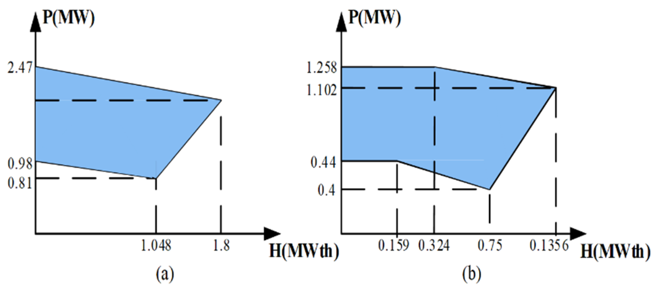
CHP units simultaneously generate electricity and heat. It means that the electricity and heat generated by the CHP units are interdependent and they cannot be controlled individually. There are two types of feasible operation regions (FOR) for CHP units [28]. Two FOR types are shown in Figure 1. FOR type I (Figure 1a) can be modeled linearly. Equations (34)–(38) describe FOR type I in the scheduling problem of this grid [28]:
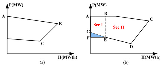
Figure 1.
Feasible operation region for CHP units, (a) type I, (b) type II.
M represents a large number, and the indices A, B, C, and D specify four boundary points of FOR type I. Equation (34) models the area below the AB line. Equation (35) formulates the upper area of the BC line, and the upper area of the CD line has been represented by Equation (36). According to Equations (35) and (36), the output power of the OFF unit will be zero. The electricity and the heat generated by the OFF unit will always be zero, which has been expressed in Equations (37) and (38) respectively. As shown in Figure 1, FOR type II is non-convex and can be divided into two convex subregions I and II. FOR type II has been specified by the closed curve of ABCDEFG. In this case, if the typical formulation type I is used, the light blue area will be ignored. This non-convex area is determined using the binary variables X1 and X2 [28]. Therefore, non-convex FOR is divided into two convex subregions I and II. The following equations have been considered for modeling the type II FOR of CHP units [28]:
In the second type, the indices A, B, C, D, E, and F show the corner points of FOR of Figure 1b. Equation (39) introduces the region below the BC line. The upper bound of the CD line has been described by Equation (40). The upper region of the DE and EF lines have been specified by Equations (41) and (42), respectively. In Equations (41)–(44), X1,t = 1 means that the CHP unit operates under the region I of FOR, and X1,t = 2 indicates that the CHP unit operates under the region II of FOR. According to Equation (45), if the CHP unit is on, it definitely works in one of regions I and II and in the case of being OFF, it does not operate in any of the regions. According to Equations (46) and (47), heat and electricity generation in OFF units is zero.
2.5.2. Constraints of Conventional Power Generation, Boilers, and Fuel Cell Units
The capacity range of power generation of a conventional electricity unit, boiler, and fuel cell can be indicated as follows [10]:
2.5.3. Wind Power Constraints
The total power generated by a wind turbine is a function of wind speed and wind turbine characteristics. In [10], the power generation by the wind turbine has been modeled as follows:
where, denotes the wind speed at time t and, , and are respectively, the minimum speed, the maximum speed, and the rated speed of the m-th turbine. Additionally, and are respectively the rated power and power generation of the m-th wind turbine. In the case of lack of need for wind power generation (based on the algorithm’s decision), the power generation is overflowed as follows:
while, is the wind power generated by turbines.
2.5.4. Solar Power Constraints
A photovoltaic (PV) converts solar energy into electrical energy. The output power of the PV module depends on the area of the solar cell, the solar radiation, the ambient temperature, and the conversion factor of the module. In order to maximize output power, it is assumed that the solar cell has been installed on an appropriate point and at an optimal angle. The output power of the PV system is expressed as follows [10]:
In the above equation, is the solar cell’s power generation, is the solar radiation, and denotes the ambient temperature at t; also, A and are respectively the solar cell area and the conversion efficiency of module. In the case of lack of need for all or a part of the solar power generation (based on the decision of the algorithm), the power generation can overflow. This is stated as follows:
where, represents the solar power that is used in the system.
2.5.5. Electrical Energy Storage Constraints
The constraint of the balance of the electrical energy storage system can be written as follows [29]:
where, and are respectively the battery charge and discharge coefficient. Similarly,, , and respectively represent the charged power in the battery, discharged power of the battery, and power stored in the battery at time t. The ranges of stored energy, the charge and discharge power in the battery are determined as follows:
The binary variables of and are respectively, the status of charging and discharging the battery. In Equations (57)–(59), means that the battery is in charge state and means the discharge state of the battery at t; also, if and , the battery is not charged or discharged. These limitations allow the battery to save energy at the hours where energy price is low and to sell it to the microgrid’s consumers or to the market at the hours where the energy price is high.
2.5.6. Heat Storage Constraints
In this paper, the model presented in [12] has been used for the heat storage system. The heat storage unit has been connected to CHP and boiler units. In this model, stored thermal energy is always available. The total heat generated is expressed by the following equations:
where, is the total thermal energy generated in the studied CHP-based microgrid. Considering that the heat storage unit is connected to the heat generation units; each time the heat generation unit is started, the heat storage unit loses energy () and each time these units shut down, the surplus heat returns to the heat storage unit (). The pure thermal energy that can be injected into the heat storage unit is equal to [30]:
Therefore, the heat stored in the heat storage unit is calculated according to equation [6]:
is the heat loss factor of the heat storage unit; also, and are respectively the heat demand of the microgrid, and the heat stored in the storage unit at time t. The heat storage capacity is limited by the following equation [6]:
The rate of heat injection to the heat storage unit and the rate of heat output is described by the following equations [30]:
2.6. Power Balance
According to the following constraint, the total power generated by the units at each hour, the power discharged from the battery, and the power purchased from the market (i.e., ) is equal to the total charged power of the battery, the power sold to the market (i.e., ), and demand (after applying the DRP):
2.7. Implementation of IGDT Method
In the proposed model for CHP-based microgrid scheduling, uncertain input parameters are the power generated by wind and solar farms. As a result, the model of the objective function constrained to the power balance in the base case is written as follows. It should be noted that in the base case, the output power of wind and solar farms is equal to the predicted value (or its estimated value).
Subject to:
(23) to (66)
In Equation (67), OFb is the net daily revenue in the base case in which the uncertain parameters are exactly equal to the corresponding predicted value. and are respectively the average power generation values of wind turbines and solar farms. Equation (68) also implies that all Equations (23)–(66) should be considered simultaneously.
Given the RA strategy presented in Section 2, at a given demand and price level, reducing the injection power of wind and solar farms from their predicted (estimated) levels would lead to increased power generation by other units, resulting in increased generation costs and decreased net daily revenue of the microgrid. Therefore, the actual output power of wind and solar farms can be expressed in terms of the corresponding predicted value by Equations (72) and (73). Ultimately, according to the explanation given earlier about the RA approach, the model of the problem constrained to the power balance is as follows:
Subject to:
(23) to (66)
Accordingly, (69) is the uncertainty radius of wind and solar power generations (as the uncertain parameters), as defined in (72) and (73). Additionally, (70) is the set of all constraints considered in the base case, as defined in (23)–(66). Furthermore, the tolerable limit of the objective function obtained in base case, i.e., OFb, is defined by (70).
3. Simulations and Results
In this section, the studied microgrid structure are first introduced; then simulation results are presented.
3.1. Structure of the Studied Microgrid
Figure 2 shows the overall layout of the microgrid under study. According to this figure, the microgrid consists of three wind turbine units, one hectare of a solar farm, two CHP units with different FORs, a conventional power generation unit, a fuel cell unit, a boiler unit, a heat storage unit, a battery energy storage unit, and electrical and heat demands.
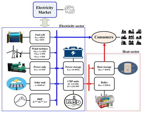
Figure 2.
The CHP-based microgrid under study.
The penetration level of the DRP is considered to be 30% (). The specifications of the battery and the heat storage unit are presented in Table 1 and Table 2, respectively [6]. The start up and shut down costs of the various units are given in Table 3 [6]. Additionally, the cost functions of the boiler, the conventional power generation unit, the fuel cell unit, and the CHP units are expressed in Equations (74)–(78), respectively [6].

Table 1.
Specification of battery energy storage unit [6].
Table 2.
Specification of heat storage unit [6].
Table 3.
Start up and shut down costs of the units [6].
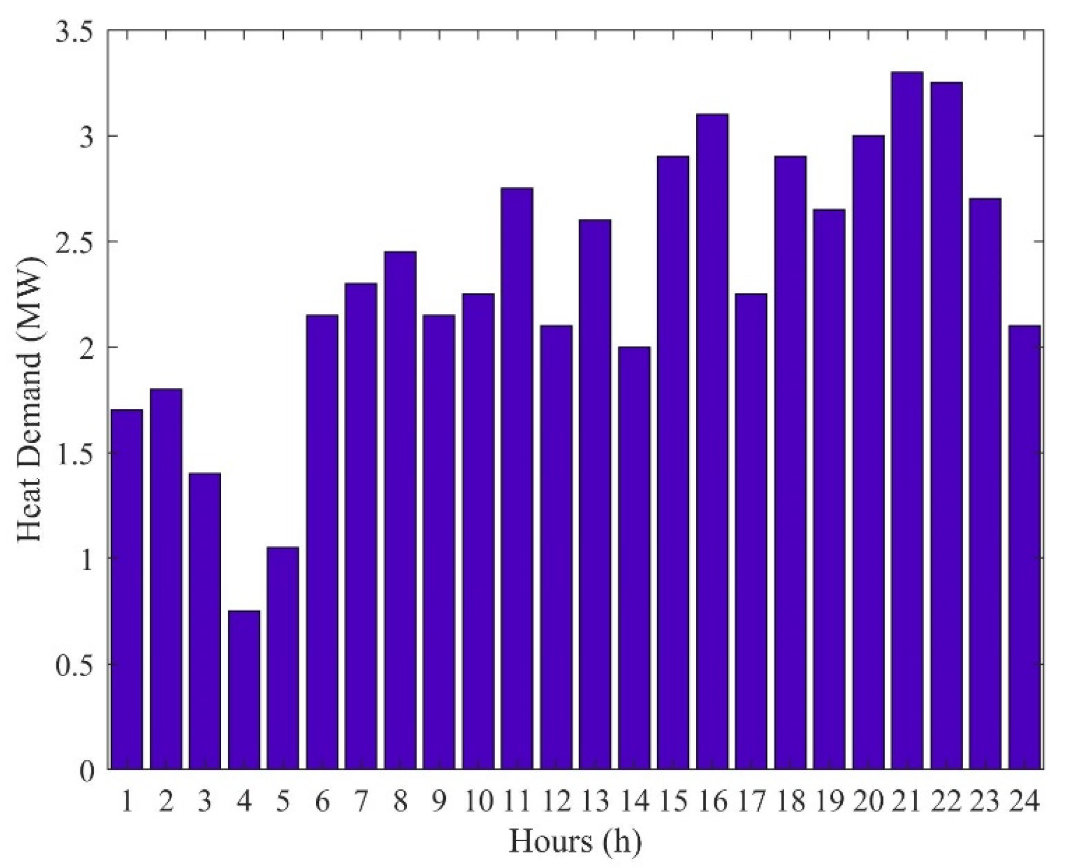
The predicted thermal energy demand of the microgrid is shown in Figure 3 [6]. The FOR of CHP units are illustrated in Figure 4 [6]. The cut-in, rated, and cut-out speeds of the wind turbines are 3.5 (m/s), 11.9 (m/s), and 25 (m/s), respectively [31]. Additionally, the rated power of the wind turbines is 1.1, 2.0, and 3.0 MW, respectively. The conversion efficiency of PV modules in (53) is assumed to be .

Figure 3.
Predicted heat demand [6].

Figure 4.
The FOR of CHP units [6], (a) type I, (b) type II.
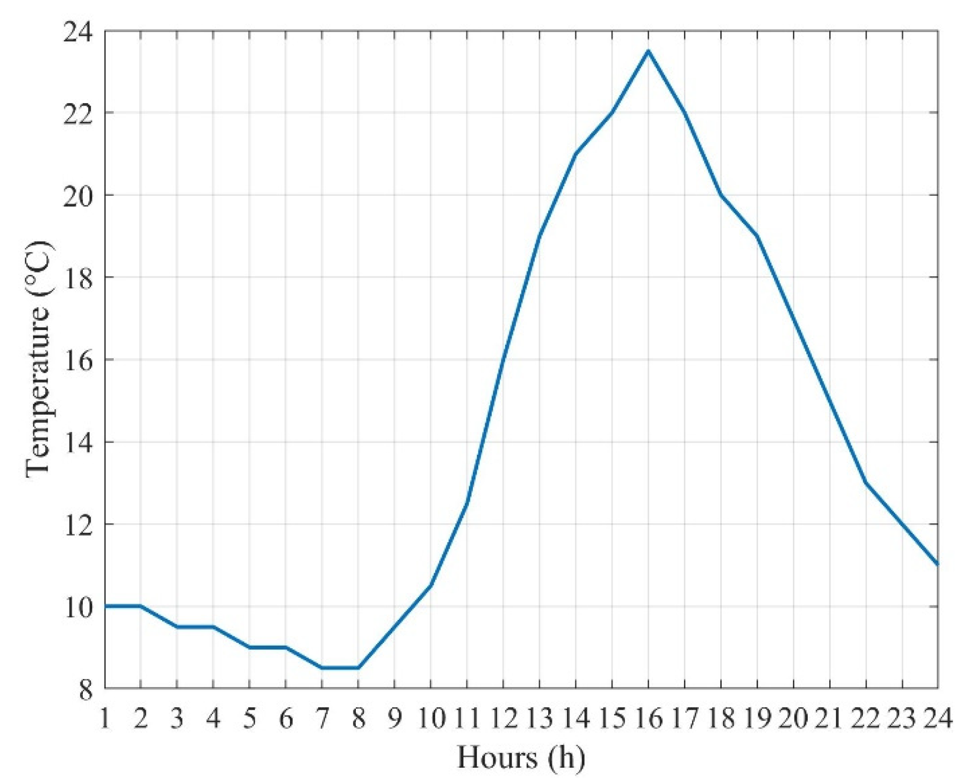
Additionally, Table 4 and Table 5 provide the mean and standard deviation of wind speed and solar radiation, respectively [32]. Figure 5 gives the average ambient temperature [32].
Table 4.
Mean and standard deviation of wind speed [32].
Table 5.
Mean and standard deviation of solar radiation [32].

Figure 5.
Average ambient temperature [32].
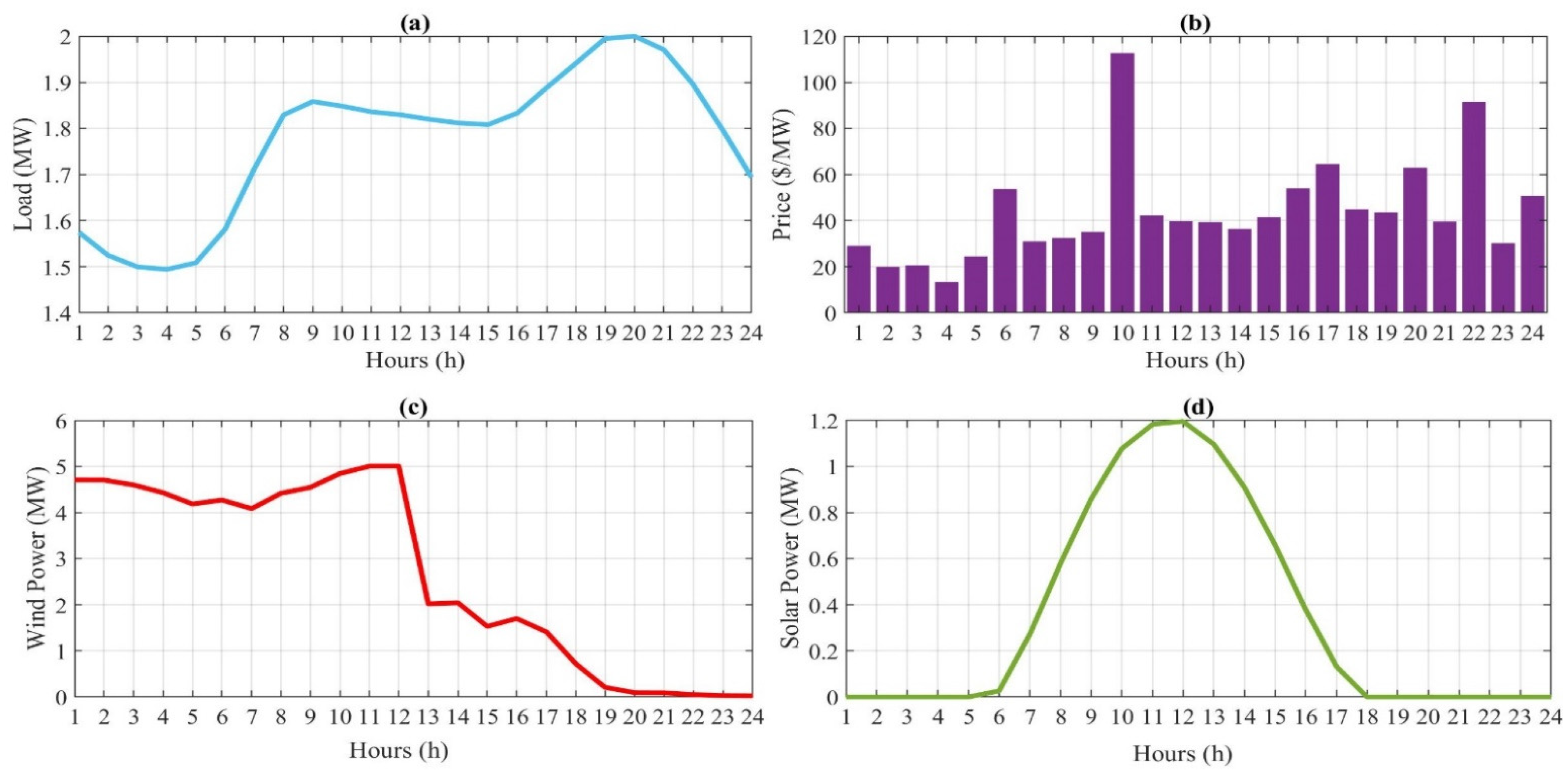
The 24 h demand and price profiles are shown in Figure 6a,b, respectively [33]. The predicted (or average) power generation values of wind and solar PV farms are also given in Figure 6c,d, respectively [32].
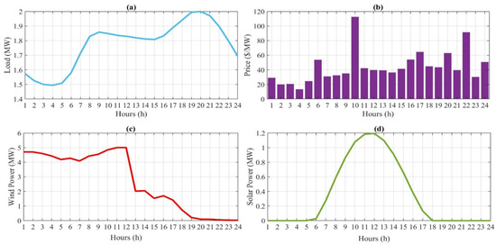
Figure 6.
Information of one sample day; (a) demand profile, (b) price of electricity market, (c) average available wind power, (d) average available solar power.
3.2. Considered Case Studies
The aforementioned CHP-based microgrid is studied in the following four different cases:
- Case 1: CHP-based microgrid scheduling in islanding (off-grid) mode in the absence of DRP.
- Case 2: Microgrid scheduling in the on-grid mode, without considering DRP capability.
- Case 3: Microgrid scheduling in the on-grid mode, considering DRP capability.
- Case 4: Microgrid scheduling in the on-grid mode, considering DRP capability via the RA strategy of the IGDT technique.
In Case 1, the microgrid is operated in off-grid mode, which means that and are both zero in (66). While in Cases 2, 3, and 4, the microgrid can exchange (purchase and sell) electricity with the main grid (or power market). Additionally, the mean values of uncertain input parameters are used in Cases 1–3.
In all cases, a robust IGDT scheduling approach is utilized. In Cases 1–3, it is assumed that the predicted values of uncertain parameters are equal to real values and only the base case is examined. In other words, the (predicted) average power generation values for wind turbines and solar farms have been used. In Case 4, the RA strategy of the IGDT method is used and the maximum uncertainty radius of the uncertain parameters is calculated. In addition, Monte Carlo simulations with 1000 repetitions for the scheduling of CHP-based microgrid are performed. In all these trial runs, the demand and price are assumed to be certain as given in Figure 6a,b while the uncertainties of wind speed, solar radiation and ambient temperature are modeled using the corresponding PDF presented in Section 2. The hourly mean and standard deviations of wind and solar power generation used in these trial runs are given in Table 4 and Table 5. It should be noted that the standard deviation of the ambient temperature is 2% of its average at each hour given in Figure 5.
The proposed optimization model for the CHP-based microgrid scheduling problem is implemented and solved using the BARON/CONOPT solver in the GAMS optimization software environment.
3.3. Simulation Results
3.3.1. Case 1
In this case, the microgrid has been scheduled in islanding mode for 24 h by the equations provided in the previous section; also, all economic constraints have been considered. Additionally, it should be noted that the DRP has not been implemented. The basic case of IGDT method has been used. In other words, it is assumed that the uncertain parameters are exactly equal to the corresponding mean values obtained from the Monte Carlo method. Table 6 presents a summary of four cases.
Table 6.
Summary of the results of the studied cases.
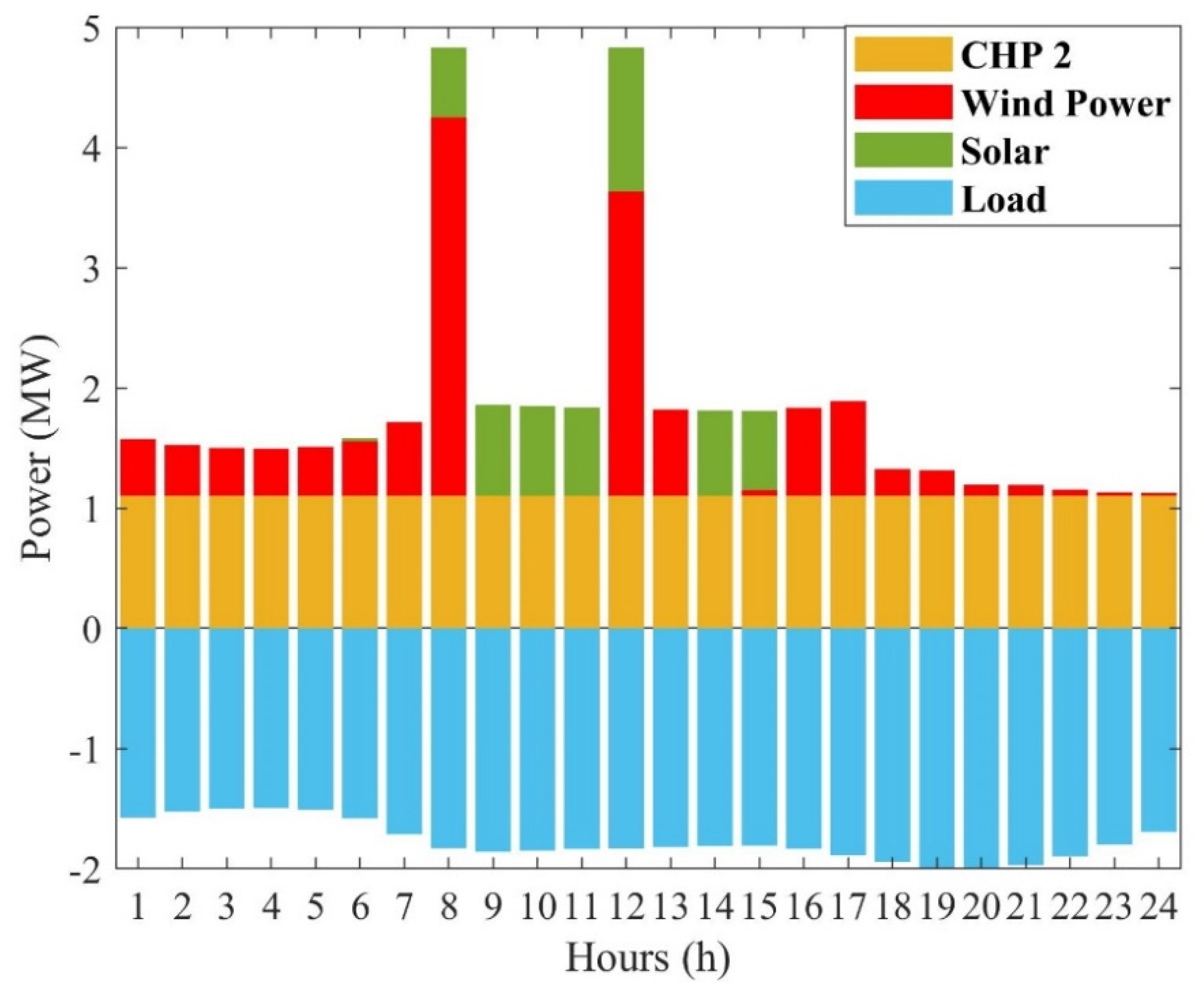
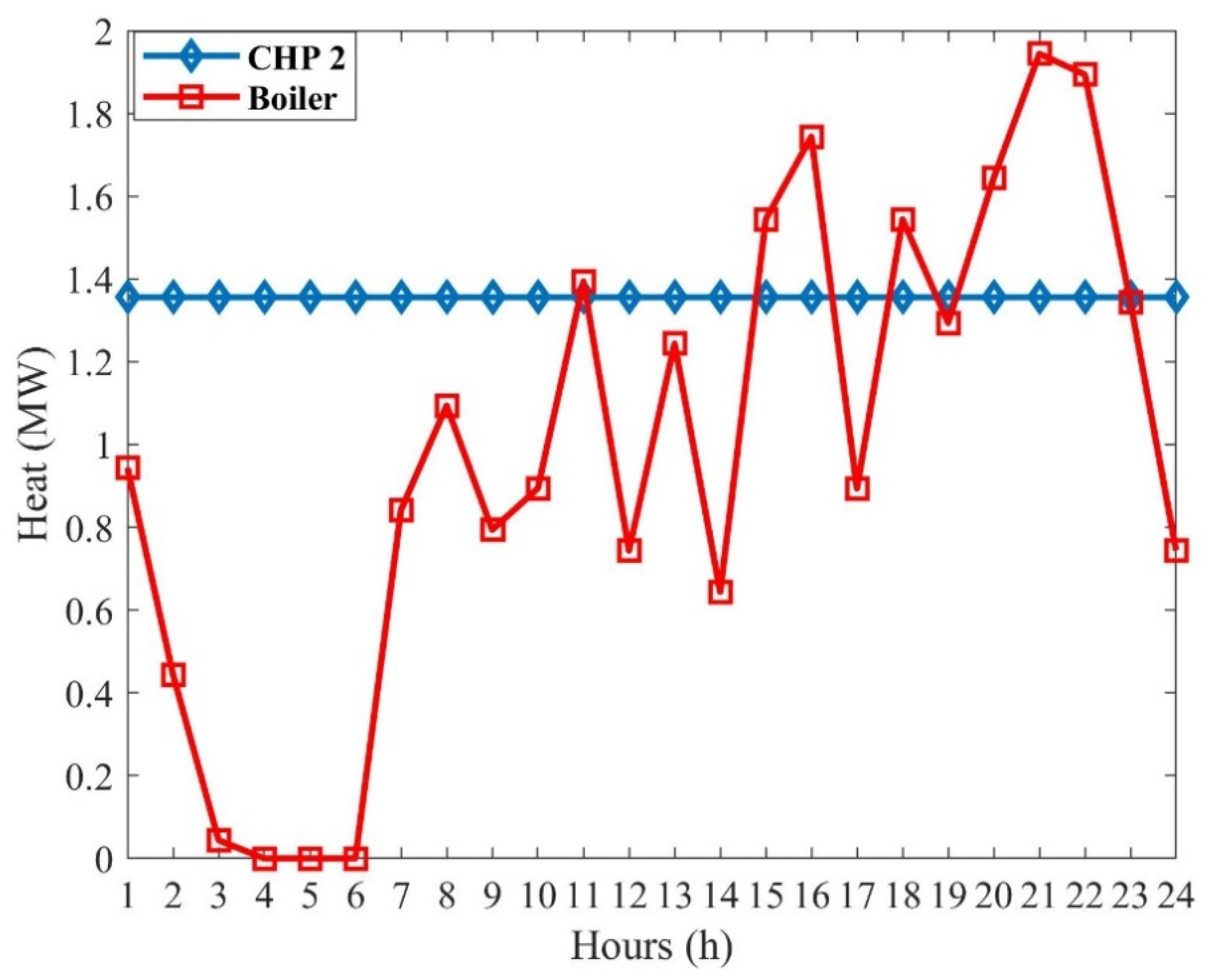
According to Table 6, the cost of electrical and thermal energy required for the microgrid in islanding mode is USD 2013.5. Figure 7 shows the results of electric power generation in the islanding mode. It is worth noting that the negative axis in this figure refers to the hourly electricity demand of the microgrid as also given in Figure 6a. According to Figure 7, CHP2, wind and solar units provide 60, 38.5, and 1.5% of the electrical energy needed for the microgrid. Figure 8 shows the results of thermal energy generation in this case. As shown in this figure, CHP2 and boiler units provide 58% and 42% of the thermal energy required by the microgrid’s heat demand. As shown in Figure 4, the generation of electric and thermal energy by the CHP unit cannot be controlled independently. Therefore, this unit generates electricity and heat simultaneously. This does not allow wind and solar units to operate at their maximum available power generation capacity (as given in Figure 6c,d); however, the cost of generating electricity by solar and wind farms is assumed to be zero.

Figure 7.
Electric power generation in Case 1.
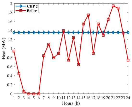
Figure 8.
Thermal energy generation in Case 1.
3.3.2. Case 2
In this case, the CHP-based microgrid is considered to be connected to the main grid, also, the effects of electrical power exchange with the main grid have been studied. All economic constraints are considered in the 24 h scheduling of the microgrid in the case of being connected to the main grid. As in the first case, in this case, the DRP has not been applied; also, the uncertain parameters are exactly equal to the mean value. According to Table 6, in the second case, the net profit of the microgrid from the market is USD 5928.1. This revenue has been obtained from the sale of surplus electricity to the main grid. In this case, generation costs increased by 69% compared to the first case. Selling surplus electricity to the main grid has earned a net profit of USD 2371.01. Figure 9 shows the electric power generation results in this case. It is noteworthy that the minus powers in this figure denote the hourly load, and the surplus production in the microgrid which is injected to the upstream power network (denoted by electricity market). As shown in Figure 9, wind and solar farms are operating at their maximum available generation capacity. The microgrid in the grid-connected mode buys electricity from the main grid at low-price hours, and in most hours, it sells surplus electricity to the main grid. According to Table 6 and Figure 9, the low cost of energy generation by CHP units can be seen. Figure 10 shows the heat generated by the CHP units and the boiler unit in this case. According to this figure, due to the higher operation cost of the boiler unit, it is not committed in the supply of thermal energy demand of the microgrid during the entire scheduling period. It is worth noting that as CHP units are participating in both electricity and heat supply, they are beneficial to be used for heat generation in this case.
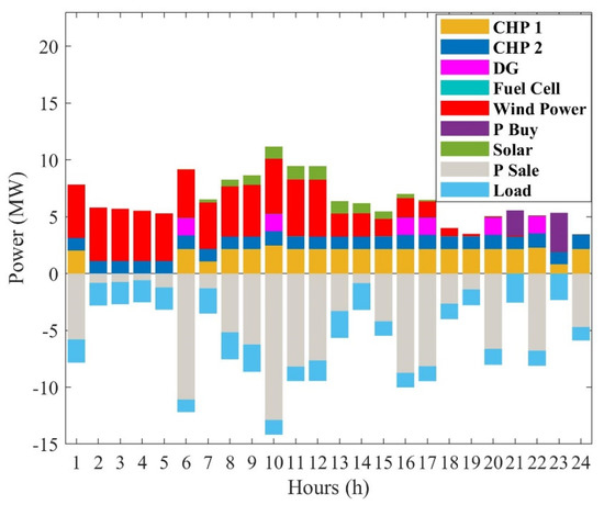
Figure 9.
Electric power generation in Case 2.
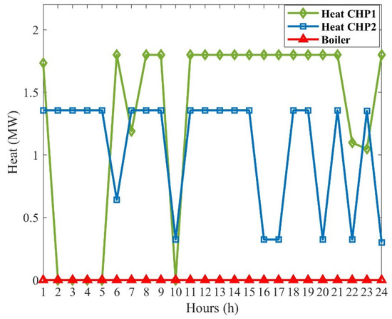
Figure 10.
Thermal energy generation in Case 2.
3.3.3. Case 3
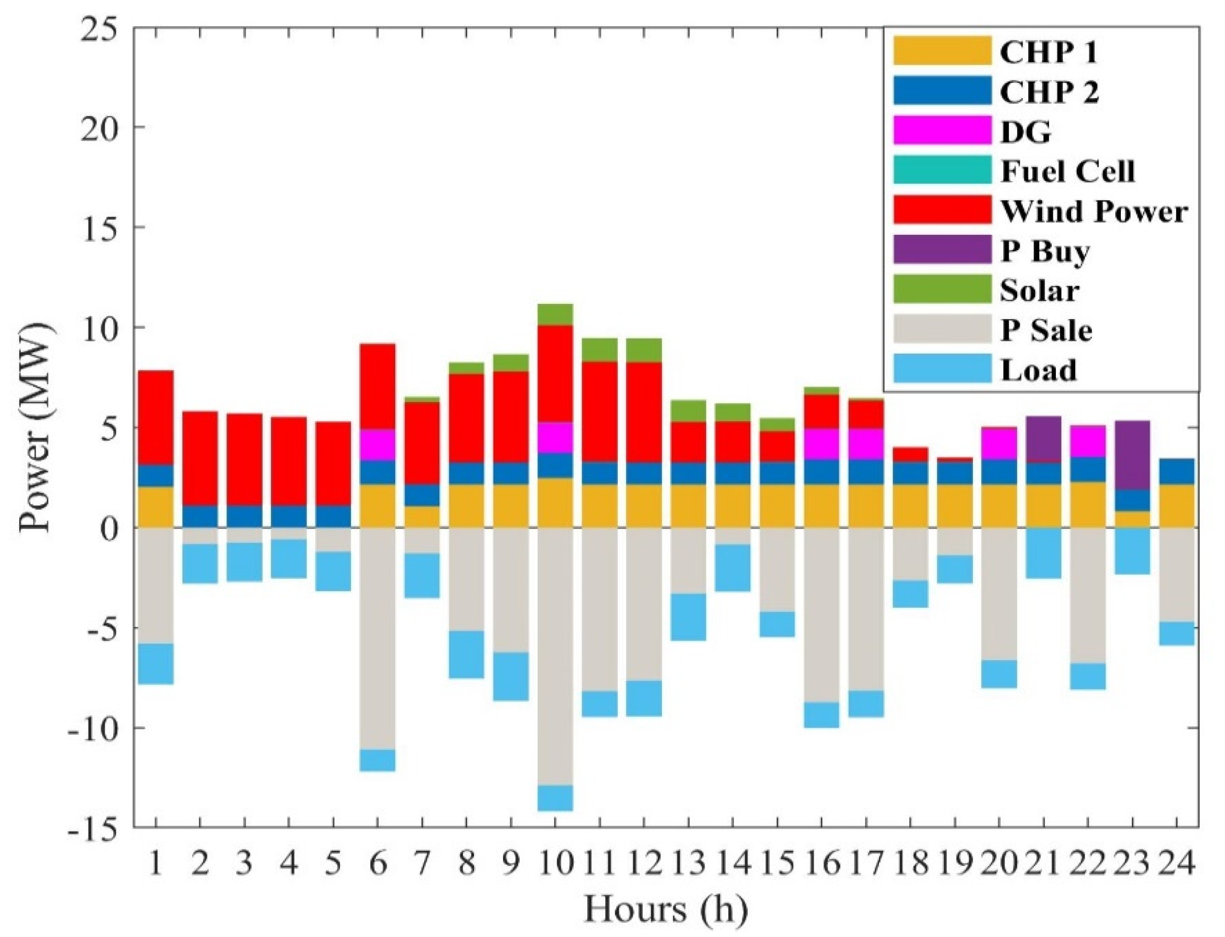
In this case, the CHP-based microgrid is considered to be connected to the main grid. All economic and generation constraints have been considered. This case is similar to the previous case, with the difference that the DRP has been applied according to the model presented in the previous section during the scheduling period in order to examine its effects. Additionally, the average (predicted) power generation of wind and solar farms have been considered. Table 6 shows that the application of the DRP increases the purchase cost of electricity from the main grid by USD 39.7. However, on the other hand, it will increase sales revenue by USD 224.9. Since the market price for a particular day is considered for all cases, the generation cost is almost the same in the cases connected to the main grid. Therefore, net daily revenue has increased by about 8% compared to the previous case. Figure 11 shows the results of electric power generation by wind, solar, DG, CHP1, CHP2, fuel cells as well as purchased, sold power, and demand at any time of the day. It is worth noting that the minus powers in this figure denote the modified hourly load profile (i.e., by applying the DRP), and the surplus production in the microgrid which is injected to the upstream power network (denoted by electricity market).

Figure 11.
Electric power generation in Case 3.
As shown in Figure 9 and Figure 11, the DRP transfers the electricity demand from the intervals with high energy price to the low-price intervals. The output heat generated by CHP and boiler units in the third case is equal to the second case (Figure 10) and the boiler does not contribute to the thermal energy required by the microgrid. This is due to the high cost of boiler operation and low operation cost of CHP units.
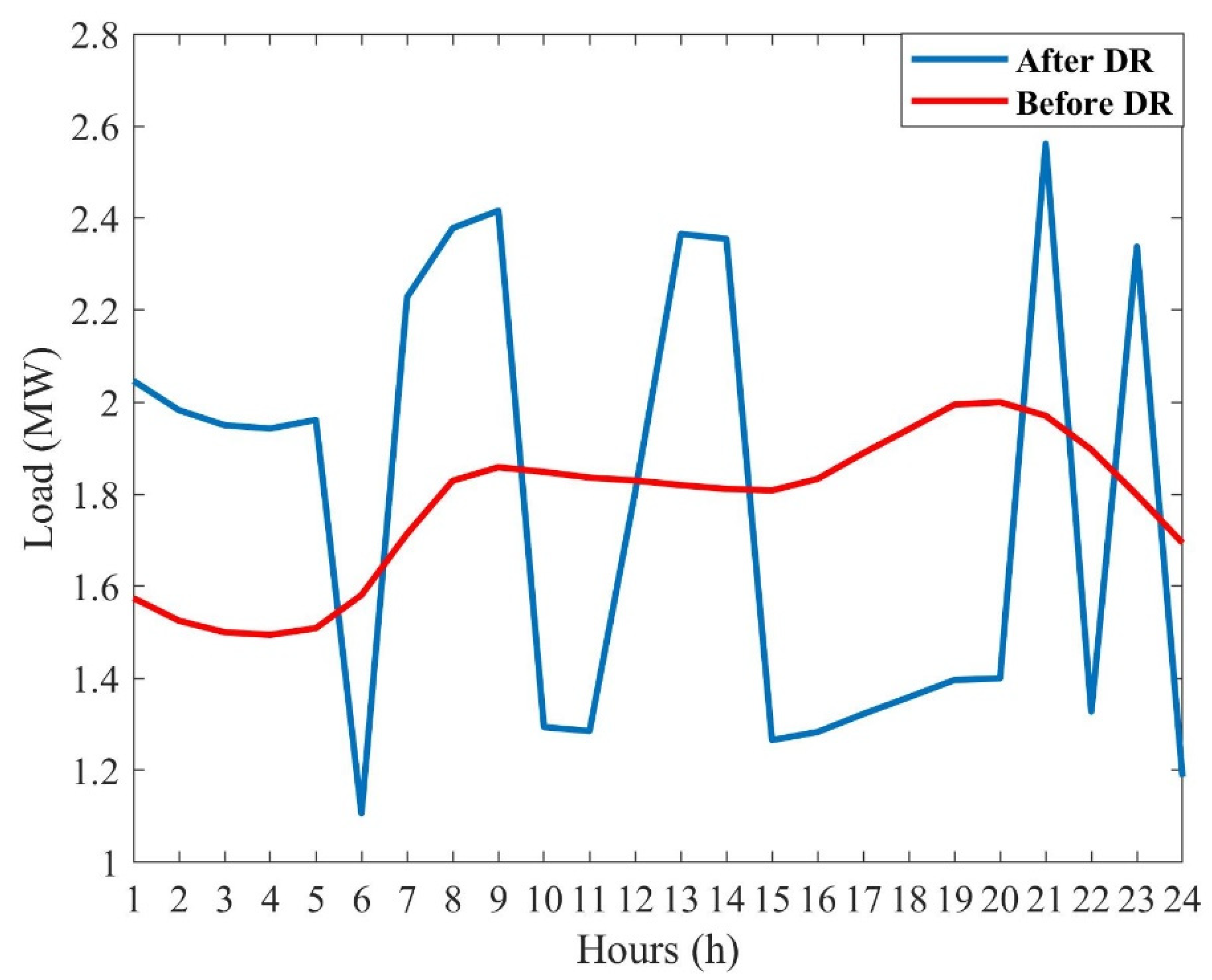
Figure 12 shows the demand profile before and after applying the DRP. It is observed from this figure that the DRP shifts the demand from higher price intervals to lower price hours. For example, based on the hourly electricity prices given in Figure 6b, there is a peak in the price at hour 10; hence a sharp drop in the demand at this instant is expected, as realized in Figure 12. Similarly, during the early morning interval, i.e., the hours 1–5, the electricity price is quite low and hence, the demand is shifted to this interval via DRP. Additionally, a high percentage of load is participating in the DR program (30% here). This leads to higher peak demands in the modified load profile. Besides, the participating loads in the DR program are constant energy loads, which means these loads are not curtailed, but shifted from peak price intervals to off-peak price intervals. If the DR percentage decreases, the demand’s peaks in the modified profile will be reduced.
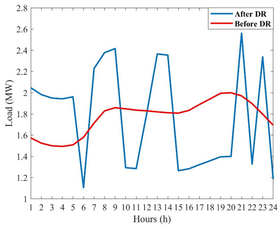
Figure 12.
Demand profiles before and after applying the DRP in Case 3.
3.3.4. Case 4
In this case, the microgrid is assumed to be connected to the main grid. All the economic constraints have been considered, in particular the DRP. The difference between this case and the previous one is that in the fourth case, the RA strategy of the IGDT method is used for 24 h scheduling horizon. In other words, instead of the predicted values (average) of uncertain parameters, the corresponding real values, which are functions of the predicted values, have been used.
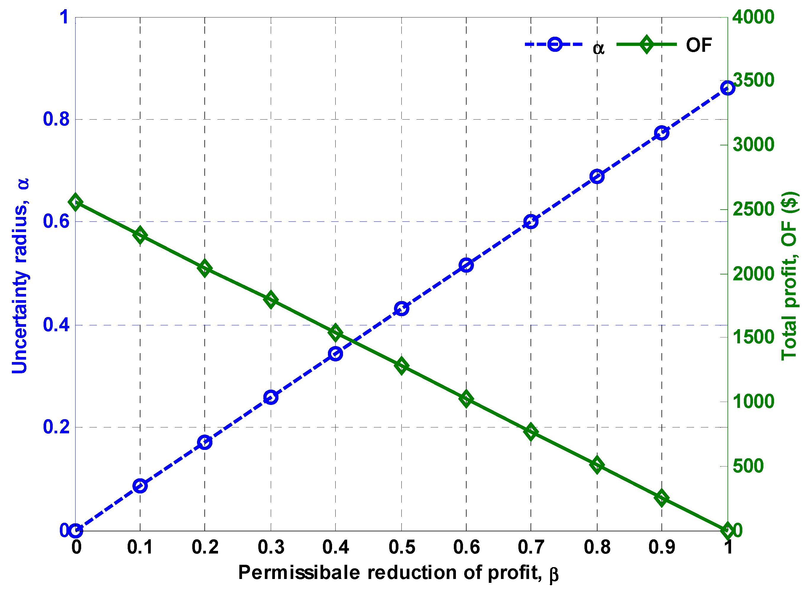
Figure 13 shows variations of uncertainty radius, i.e., α and total profit, i.e., OF versus β. It is worth mentioning that β, which is the maximum permissible reduction of OF subject to the uncertainty, is preset by the decision maker. In the microgrid scheduling, a certain value of β maximizes α. As shown in Figure 13, by increase of β the uncertainty radius, i.e., α increases, while the OF decreases with respect to its value in base case, i.e., OFb. When β equals 1.00, the OF is zero and α is equal to 0.86. In other words, with the scheduling provided in this paper, the CHP-based microgrid can compensate the cost of energy supply by selling surplus electricity to the main grid, with only 14% of renewable resources. According to the equations presented in the previous section, it can be said that α is a criterion for measuring the robustness of the microgrid scheduling against the uncertainty of the uncertain parameters.
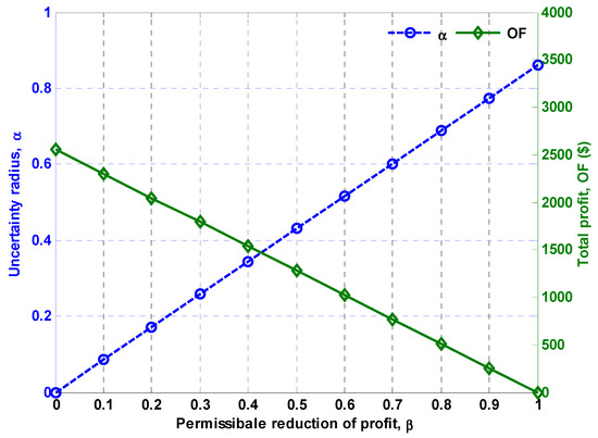
Figure 13.
Variation of α and OF vs. β.
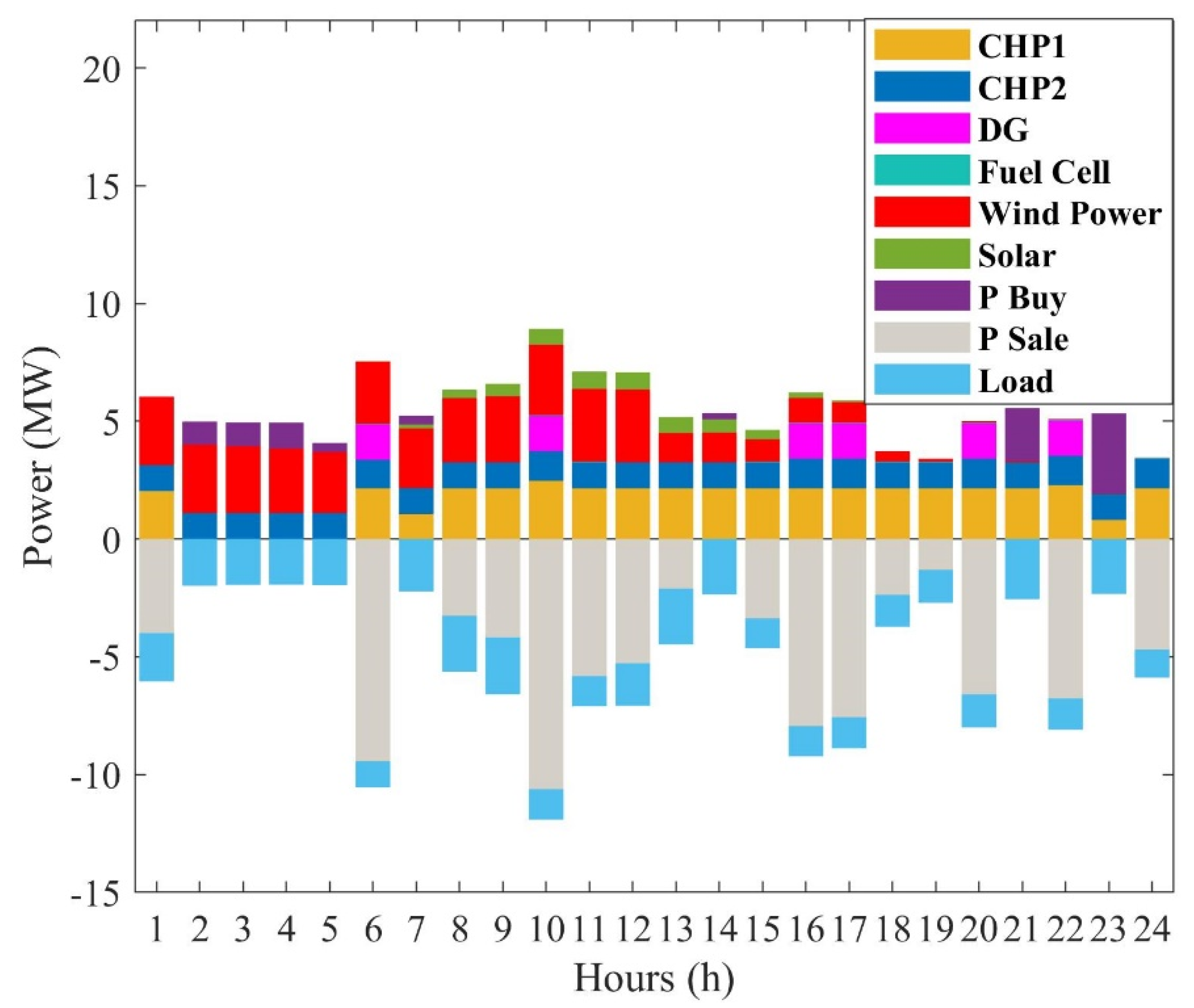
Figure 14 shows the results of the microgrid schedule for β = 0.40. In this case, the value of α will be 0.34. This means that the power generation by wind and solar farms is 34% lower than the average value. By reducing 34% of the power generation by renewable resources, according to Table 6, net microgrid revenue will decrease by 40%. According to Table 6, in this case, the power purchased from the main grid has increased by about USD 65 compared to Case 3; whereas, the sales have decreased by about USD 958.

Figure 14.
Electric power generation in Case 4 (for β = 0.4).
3.3.5. Monte Carlo Simulations (MCS)
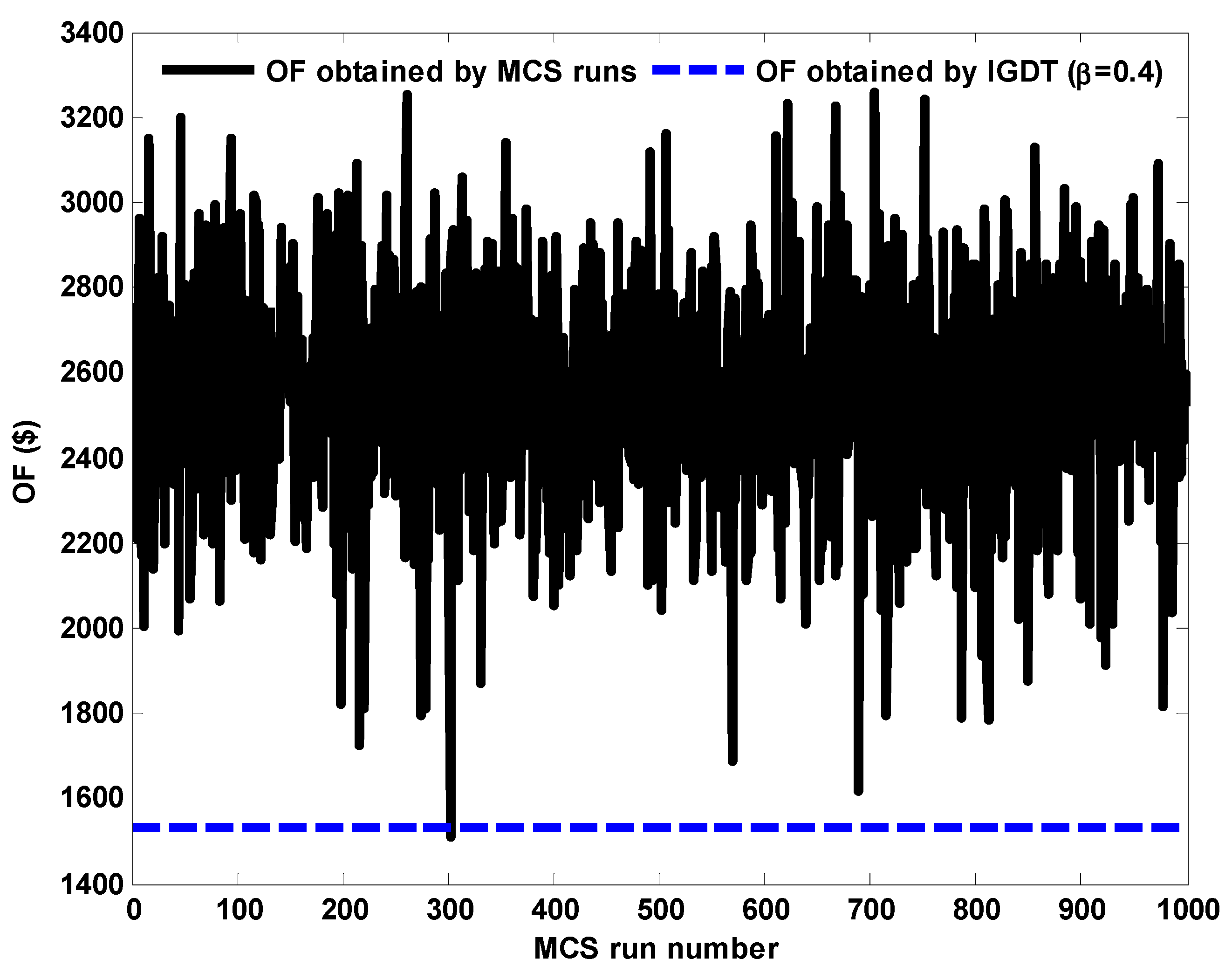
In this section, 1000 runs of MCS are done for CHP-based microgrid scheduling. Uncertain parameters are modeled by the corresponding PDF presented in the previous section. In Figure 15, the net profit obtained from 1000 repetitions of the MCS is compared with the profit obtained by the RA strategy of the IGDT method with a hypothesized value of β = 0.4, i.e., USD 1533.89. According to this figure, the profit derived from the RA strategy is lower than the overall benefit rate of all MCS replications. Given that α is the maximum allowable uncertainty radius of the uncertain parameters for the given β = 0.4, α is equal to 34%. It can be concluded that, in the worst-case conditions, the daily electric power generation by renewable resources will not be less than 66% of the corresponding forecasted values given in Figure 6c,d. The average profit earned by the MCS method is USD 2556.49 and the standard deviation is USD 255. If the uncertainty of wind and solar power generation is zero, the benefit obtained by the IGDT is almost the same with the mean OF obtained by the MCS, as shown in Figure 13 for β = 0.0. However, for the higher levels of permissible uncertainties (corresponding to higher levels of β), the profit obtained by the MCS is higher than that obtained by the IGDT technique.
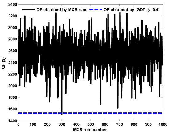
Figure 15.
Comparison between daily net revenue of the MCS and IGDT methods.
4. Conclusions
This paper proposed a robust day-ahead scheduling model for CHP-based microgrids at the presence of severe uncertainties of renewable energy sources. A RA strategy based on IGDT technique is developed aiming to determine the maximum allowable uncertainty radius for the output power of renewable energy sources, for a predetermined limit on the reduction of the revenue of all participants in the microgrid energy supply. The conclusions are summarized as follows.
- For a given level of β, i.e., β = 0.4 the uncertainty radius, i.e., α is obtained to be 0.34. This means that, with the consent of the 40% reduction in the objective function relative to its base-case value, at least 66% of the predicted amount of power generation by renewable energy sources could be available.
- By considering random variations of uncertain parameters based on their corresponding PDFs, via MCS trials, it is observed that the obtained schedule for the microgrid is robust for the determined radius of uncertainty.
- The robust schedule of the microgrid is obtained without any information regarding the nature and behavior of uncertain parameters, e.g., their PDF.
- Additionally, despite the other methods for uncertainty handling, such as MCS and scenario-based stochastic modeling, the IGDT does not add any computational complexity to the scheduling problem of microgrids.
Author Contributions
Conceptualization, M.H. and A.R.; methodology, M.H. and A.R.; software, M.H. and S.M.M.-B.; validation, A.A. and S.M.M.-B.; formal analysis, M.H., A.A. and A.R.; investigation, A.A., S.M.M.-B. and A.R.; resources, A.R.; data curation, A.A.; writing—original draft preparation, A.A.; writing—review and editing, A.R.; visualization, A.A. and S.M.M.-B.; supervision, A.R.; project administration, A.R. All authors have read and agreed to the published version of the manuscript.
Funding
This research received no external funding.
Data Availability Statement
Data are contained within the article.
Conflicts of Interest
The authors declare no conflict of interest.
Nomenclature
| Alphabetic symbols | |
| a, b, c, d, e, f | CHP unit cost function coefficients |
| A | Area of solar farm ) |
| B | Heat stored in the storage unit |
| C | Cost of the unit’s operation |
| c | Scale parameter of Weibull PDF |
| DL | Percentage of decreasing demand |
| E | Battery stored power |
| H | Heat generated (MW) |
| IL | Percentage of increasing demand |
| k | Form parameter of Weibull PDF |
| P | Power generation and demand |
| s | Solar radiation |
| SU | Startup status of the units |
| SD | Shut down status of the units |
| T | Ambient Temperature (°C) |
| V | Binary variable indicator of ON and OFF status of the units |
| Greek symbols | |
| Maximum possible deviation of the uncertain parameter | |
| Degree of tolerance of the reduction of the OF | |
| Parameters of the beta function | |
| Uncertain input parameter | |
| Cost function coefficient of a fuel cell | |
| Price of electricity market | |
| Mean | |
| Cost function coefficient of a boiler | |
| Standard deviation | |
| Wind speed | |
| Set of decision-making variables | |
| Set of uncertainties | |
| Gamma function | |
| Critical value of objective function | |
| Uncertainty radius of the uncertain parameter | |
| Cost function coefficient of a conventional power generation unit | |
| Subscripts | |
| cha | Battery charging |
| discha | Battery discharging |
| gain | Heat return |
| loss | Energy losses |
| h | Total number of power generation units |
| i | Number of CHP units |
| j | Number of conventional power generation units |
| k | Number of boiler units |
| l | Number of fuel cell units |
| m | Number of wind turbines |
| t | Time (Hour) |
| Superscript | |
| CHP | CHP unit |
| CI, CO, R | Minimum, maximum, rated wind speed |
| inc | Transferred demand from the other hours to t |
| dec | Transferred demand from t to the other hours |
| WT | Wind turbine |
| 0 | Microgrid demand before applying the DRP |
| B | Fuel cell unit |
| F | Boiler unit |
| P | Conventional power generation unit |
| T | Temperature |
| s | Solar radiation |
References
- Yaprakdal, F.; Yılmaz, M.B.; Baysal, M.; Anvari-Moghaddam, A. A Deep Neural Network-Assisted Approach to Enhance Short-Term Optimal Operational Scheduling of a Microgrid. Sustainability 2020, 12, 1653. [Google Scholar] [CrossRef]
- Ramli, M.A.M.; Bouchekara, H.R.E.H.; Alghamdi, A.S. Efficient Energy Management in a Microgrid with Intermittent Renewable Energy and Storage Sources. Sustainability 2019, 11, 3839. [Google Scholar] [CrossRef] [Green Version]
- Wang, Y.; Huang, Y.; Wang, Y.; Li, F.; Zhang, Y.; Tian, C. Operation Optimization in a Smart Micro-Grid in the Presence of Distributed Generation and Demand Response. Sustainability 2018, 10, 847. [Google Scholar] [CrossRef] [Green Version]
- Dagdougui, Y.; Ouammi, A.; Benchrifa, R. Energy Management-Based Predictive Controller for a Smart Building Powered by Renewable Energy. Sustainability 2020, 12, 4264. [Google Scholar] [CrossRef]
- Wang, J.; Wu, C.; Niu, T. A Novel System for Wind Speed Forecasting Based on Multi-Objective Optimization and Echo State Network. Sustainability 2019, 11, 526. [Google Scholar] [CrossRef] [Green Version]
- Alipour, M.; Mohammadi-Ivatloo, B.; Zare, K. Stochastic scheduling of renewable and CHP-based microgrids. IEEE Trans. Ind. Inform. 2015, 11, 1049–1058. [Google Scholar] [CrossRef]
- Bui, V.-H.; Hussain, A.; Kim, H.-M. A multiagent-based hierarchical energy management strategy for multi-microgrids considering adjustable power and demand response. IEEE Trans. Smart Grid 2018, 9, 1323–1333. [Google Scholar] [CrossRef]
- Tang, J.; Ding, M.; Lu, S.; Li, S.; Huang, J.; Gu, W. Operational flexibility constrained intraday rolling dispatch strategy for CHP microgrid. IEEE Access 2019, 7, 96639–96649. [Google Scholar] [CrossRef]
- Chaouachi, A.; Kamel, R.M.; Andoulsi, R.; Nagasaka, K. Multi objective intelligent energy management for a microgrid. IEEE Trans. Ind. Electron. 2013, 60, 1688–1699. [Google Scholar] [CrossRef]
- Mohammadi, S.; Soleymani, S.; Mozafari, B. Scenario-based stochastic operation management of microgrid including wind, photovoltaic, micro-turbine, fuel cell and energy storage devices. Int. J. Electr. Power Energy Syst. 2014, 54, 525–535. [Google Scholar] [CrossRef]
- Aluisio, B.; Dicorato, M.; Forte, G.; Trovato, M. An optimization procedure for Microgrid day-ahead operation in the presence of CHP facilities. Sustain. Energy Grids Netw. 2017, 11, 34–45. [Google Scholar] [CrossRef]
- Kopanos, G.M.; Georgiadis, M.C.; Pistikopoulos, E.N. Energy production planning of a network of micro combined heat and power generators. Appl. Energy 2013, 102, 1522–1534. [Google Scholar] [CrossRef]
- Rajabi, F.; Salami, A.; Azimi, M. Hierarchical and multi-level demand response programme considering the flexibility of loads. IET Gener. Transm. Distrib. 2020, 14, 1051–1061. [Google Scholar] [CrossRef]
- Gholizadeh, A.; Rabiee, A.; Fadaeinedjad, R. A scenario-based voltage stability constrained planning model for integration of large-scale wind farms. Int. J. Electr. Power Energy Syst. 2019, 105, 564–580. [Google Scholar] [CrossRef]
- Li, C.; Jia, X.; Zhou, Y.; Li, X. A microgrids energy management model based on multi-agent system using adaptive weight and chaotic search particle swarm optimization considering demand response. J. Clean. Prod. 2020, 262, 121247. [Google Scholar] [CrossRef]
- Li, H.; Wan, Z.; He, H. Real-Time Residential Demand Response. IEEE Trans. Smart Grid 2020, 11, 4144–4154. [Google Scholar] [CrossRef]
- Wang, Z.; Paranjape, R.; Chen, Z.; Zeng, K. Layered stochastic approach for residential demand response based on real-time pricing and incentive mechanism. IET Gener. Transm. Distrib. 2020, 14, 423–431. [Google Scholar] [CrossRef]
- Kazemi, M.; Mohammadi-Ivatloo, B.; Ehsan, M. Risk-based bidding of large electric utilities using information gap decision theory considering demand response. Electr. Power Syst. Res. 2014, 114, 86–92. [Google Scholar] [CrossRef]
- Ilbahar, E.; Cebi, S.; Kahraman, C. A state-of-the-art review on multi-attribute renewable energy decision making. Energy Strat. Rev. 2019, 25, 18–33. [Google Scholar] [CrossRef]
- Soroudi, A.; Ehsan, M. IGDT based robust decision making tool for DNOs in load procurement under severe uncertainty. IEEE Trans. Smart Grid 2013, 4, 886–895. [Google Scholar] [CrossRef] [Green Version]
- Soroudi, A.; Rabiee, A.; Keane, A. Information gap decision theory approach to deal with wind power uncertainty in unit commitment. Electr. Power Syst. Res. 2017, 145, 137–148. [Google Scholar] [CrossRef] [Green Version]
- Wu, Y.; Chu, H.; Xu, C. Risk assessment of wind-photovoltaic-hydrogen storage projects using an improved fuzzy synthetic evaluation approach based on cloud model: A case study in China. J. Energy Storage 2021, 38, 102580. [Google Scholar] [CrossRef]
- Nojavan, S.; Mohammadi-Ivatloo, B.; Zare, K. Optimal bidding strategy of electricity retailers using robust optimisation approach considering time-of-use rate demand response programs under market price uncertainties. IET Gener. Transm. Distrib. 2015, 9, 328–338. [Google Scholar] [CrossRef]
- Abapour, S.; Mohammadi-Ivatloo, B.; Hagh, M.T. Robust bidding strategy for demand response aggregators in electricity market based on game theory. J. Clean. Prod. 2020, 243, 118393. [Google Scholar] [CrossRef]
- Zare, K.; Moghaddam, M.P.; El Eslami, M.K.S. Demand bidding construction for a large consumer through a hybrid IGDT-probability methodology. Energy 2010, 35, 2999–3007. [Google Scholar] [CrossRef]
- Majidi, M.; Mohammadi-Ivatloo, B.; Soroudi, A. Application of information gap decision theory in practical energy problems: A comprehensive review. Appl. Energy 2019, 249, 157–165. [Google Scholar] [CrossRef] [Green Version]
- Moradi-Dalvand, M.; Nazari-Heris, M.; Mohammadi-Ivatloo, B.; Galavani, S.; Rabiee, A. A Two-Stage Mathematical Programming Approach for the Solution of Combined Heat and Power Economic Dispatch. IEEE Syst. J. 2019, 14, 2873–2881. [Google Scholar] [CrossRef]
- Geem, Z.W.; Cho, Y.H. Handling non-convex heat-power feasible region in combined heat and power economic dispatch. Int. J. Electr. Power Energy Syst. 2012, 34, 171–173. [Google Scholar] [CrossRef]
- Kelly, J.J.; Leahy, P.G. Sizing battery energy storage systems: Using multi-objective optimisation to overcome the investment scale problem of annual worth. IEEE Trans. Sustain. Energy 2019, 11, 2305–2314. [Google Scholar] [CrossRef]
- Gladysz, B.; Kluczek, A. A framework for strategic assessment of far-reaching technologies: A case study of Combined Heat and Power technology. J. Clean. Prod. 2017, 167, 242–252. [Google Scholar] [CrossRef]
- Orfanos, G.A.; Georgilakis, P.S.; Hatziargyriou, N.D. Transmission expansion planning of systems with increasing wind power integration. IEEE Trans. Power Syst. 2013, 28, 1355–1362. [Google Scholar] [CrossRef]
- Kayal, P.; Chanda, C.K. Optimal mix of solar and wind distributed generations considering performance improvement of electrical distribution network. Renew. Energy 2015, 75, 173–186. [Google Scholar] [CrossRef]
- Independent Electricity System Operator (IESO). Ieso.ca. [Online]. 2015. Available online: https://www.ieso.ca/ (accessed on 19 June 2021).


Publisher’s Note: MDPI stays neutral with regard to jurisdictional claims in published maps and institutional affiliations. |
© 2021 by the authors. Licensee MDPI, Basel, Switzerland. This article is an open access article distributed under the terms and conditions of the Creative Commons Attribution (CC BY) license (https://creativecommons.org/licenses/by/4.0/).