Article

Examining Land Use/Land Cover Change and Its Prediction Based on a Multilayer Perceptron Markov Approach in the Luki Biosphere Reserve, Democratic Republic of Congo

1
School of Forestry, Northeast Forestry University, Harbin 150040, China
2
Key Laboratory of Sustainable Forest Ecosystem Management-Ministry of Education, School of Forestry, Northeast Forestry University, Harbin 150040, China
3
Department of Natural Resources Management, Faculty of Agricultural Sciences, University of Kinshasa, 117 Kinshasa, Democratic Republic of the Congo
*
Author to whom correspondence should be addressed.
Sustainability 2021, 13(12), 6898; https://doi.org/10.3390/su13126898
Submission received: 14 May 2021 / Revised: 14 June 2021 / Accepted: 15 June 2021 / Published: 18 June 2021

Abstract

:
Villages within the Luki Biosphere Reserve and the surrounding cities have undergone rapid demographic growth and urbanization that have impacted the reserve’s natural landscape. However, no study has focused on the spatiotemporal analysis of its land use/land cover. The present research aims at providing a comprehensive analysis of land use/land cover change in the Luki Biosphere Reserve from the year 1987 to 2020, and to predict its future change for the year 2038. Landsat images were classified in order to provide land use/land cover maps for the years 1987, 2002, 2017 and 2020. Based on these maps, change detection, gradient direction, and landscape metric analyses were performed. In addition, land use/land cover change prediction was carried out using the Multilayer Perceptron Markov model. The results revealed significant land use/land cover changes in the Luki Biosphere Reserve during the study period. Indeed, tremendous changes in the primary forest, which lost around 17.8% of its total area, were noted. Other classes, notably savannah, secondary forest, built-up area, fallow land and fields had gained 79.35, 1150.36, 67.63, 3852.12 hectares, respectively. Based on the landscape metric analysis, it was revealed that built-up areas and fallow land and fields experienced an aggregation trend, while other classes showed disaggregation and fragmentation trends. Analysis further revealed that village expansion has significantly affected the process of land use/land cover change in the Luki Biosphere Reserve. However, the prediction results revealed that the primary forest will continue to increase while built-up area, fallow land and fields will follow a trend similar to a previous one. As for secondary forest and savannah, the forecast revealed a decrease of the extent during the period extending from 2020 to 2038. The present findings will benefit the decision makers, particularly in the sustainable natural resources management of the Luki Biosphere Reserve.

1. Introduction

Since the International Geosphere and Biosphere Program (IGBP) and the International Human Dimensions Program (IHDP) on global change initiated a research program on land use/land cover change, numerous studies in this field have been conducted at a global scale due to current issues in climate and global change [1]. The concept of land use/land cover is comprised of two dimensions: land cover, which describes the physical state or the surface of the soil (the type of vegetation, water, and soil), and land use, which illustrates the way human beings utilize the land. Land use relates to different activities that are undertaken on lands, including agriculture, pasture, or settlement [2,3,4]. A change in land cover can involve the conversion of forest to cropland or a transition from forest to settlement. Due to rapid economic development, land uses are subject to fast changes resulting in contrasting variation between different categories of land use [5]. For centuries, large areas of the terrestrial surface have experienced the LUC change [6,7].
According to Ouedraogo et al. [8] vast areas of tropical forest are converted to cropland in order to provide sufficient products to populations living in those regions. In the Democratic Republic of Congo (DRC), dense forests occupy around 115 million hectares, accounting for approximately 60% of Africa’s dense forests [9]. Unfortunately, the high rate of demographic growth, poverty, and unsustainable forest resources management by local communities have negatively impacted the environment and particularly forest resources. Meanwhile, more than 40 million people depend on forest resources for their survival [10]. However, agriculture remains the main cause of deforestation, followed by the expansion of infrastructures and the development of industrial or artisanal logging and fuel wood [11]. In addition, lack of effective policies on land use in the DRC has resulted in deforestation and degradation of forest land. Thus, the DRC experiences tremendous losses of forest area each year due to those various anthropogenic pressures [12]. The annual rate of deforestation varies from 0.18 to 0.46%, depending on the estimation methods used, types of vegetation under consideration, sites, and period under study [13,14,15,16]. Furthermore, there is still a lack of case studies on LUC change at a local scale, even though this information could be of great importance for sustainable planning of natural resources at the local level. The present study examines the LUC change in the Luki Biosphere Reserve, one of the three biosphere reserves in the DRC. It is located where there is rapid deforestation resulting from human activities intended to support the increased demand for crop products in the region and its surroundings. The Luki Reserve was created in 1979 and has been experiencing human pressure that threatens its natural landscape. The reserve is located at the crossroads of two very important roads (Matadi-Boma and Boma-Tshela), where it is prone to intensive movement of goods and people. Due to its geographic location, the reserve is subject to overexploitation [17]. The traditional exploitation (gathering of forest products, agriculture, hunting) and industrial exploitation (logging) of the environment have dramatically damaged the integrity of the reserve [18]. According to Gata [19], population growth in the Luki region has resulted in increased pressure on the forest and natural resources to meet the demand for basic food products and domestic energy. This has contributed to the erection of 21 illegal villages, in and around the reserve. According to Nyange [20], the traditional practices of agriculture constitute the main causes of the deforestation in the Luki Biosphere Reserve. Indeed, the author reports that the local communities of the reserve continuously depend on conversion of forest lands to farms in order to increase agricultural yields. This has resulted in considerable losses of forest lands over the years.
To better solve these issues, a comprehensive understanding of the previous LUC changes is required. However, despite degradation and loss of forest land being a critical issue in the region, there are still no related studies that have been conducted in the region. This further demonstrates the urgent need to provide reliable information to policy makers to enable them to develop effective strategies necessary to achieve sustainable management goals for natural resources in the region. Therefore, the present study aims at deeply examining the trends in LUC change in the region and predicting its future trends in case no actions or mitigation initiatives are implemented. Given that LUC changes are generally induced by a number of internal and external drivers that are subject to dynamic interaction with their surrounding environment, modeling based statistical equations for LUC changes may not be sufficient. Numerous methods have frequently been used to predict LUC change, including empirical models [21], evolutionary models [22], the multiple layer perceptron neural network (MLPNN)-based cellular automata model [23], the cellular automaton (CA)-Markov chain model (MCM) [24,25], and agent-based models [26]. Different authors have provided comprehensive explanations of these models [27,28]. According to Mishra et al. [29] and Feng et al. [30], these modeling approaches have been found to provide accurate information on LUC change to facilitate the policy-making process in elaborating good strategies in land use planning. On the other hand, the National Research Council [31] has shown that each of these models has its strengths and limitations in predicting LUC change. Therefore, there is need for an integrated approach by these models to overcome the corresponding limitations [27]. Recent studies have integrated a number of prediction methods to simulate LUC change [32,33]. In the present study, the MLPNN-based MCM was used to simulate the future LUC change. The MLPNN-MCM integrates both multiple layer perceptron neural network and Markovian chain model and has been successfully used in various studies [34,35]. Stochastic Markov and multiple layer perceptron neural network techniques appear to provide better prediction results on LUC change compared to the regression models [29,36,37] due to the ability of the MLPNN to predict several transitions simultaneously. MCM can automatically generate numerous parameter values that take a small number of data for training and reduce the calibration time of the model [38]. In addition, it can combine various parameters that can impact the numerous LUC transitions [27,29]. In addition, the MCM also provides the transition potentials of each LUC class to simulate the future LUC changes based on previous changes [39,40].
The goals of the present study are to: (1) examine and quantify land use/land cover change of the Luki Biosphere Reserve, and for all typical zones, including Core zone, Buffer zone, and transition zone; (2) depict spatiotemporal characteristics of village expansion in the reserve and its impacts on land use/land cover change; (3) analyze landscape pattern change of these villages; (4) predict future trends of land use/land cover change in the reserve. From a management standpoint, the present study will provide insights on previous LUC change and its future trends in the Luki Biosphere Reserve. The resulting information can help decision makers to solve issues that may arise, including whether forest losses will increase due to the increase of inhabitants in the region. This can help to elaborate effective strategies of land use management for sustainable development of the region.

2. Materials and Methods

2.1. Study Area

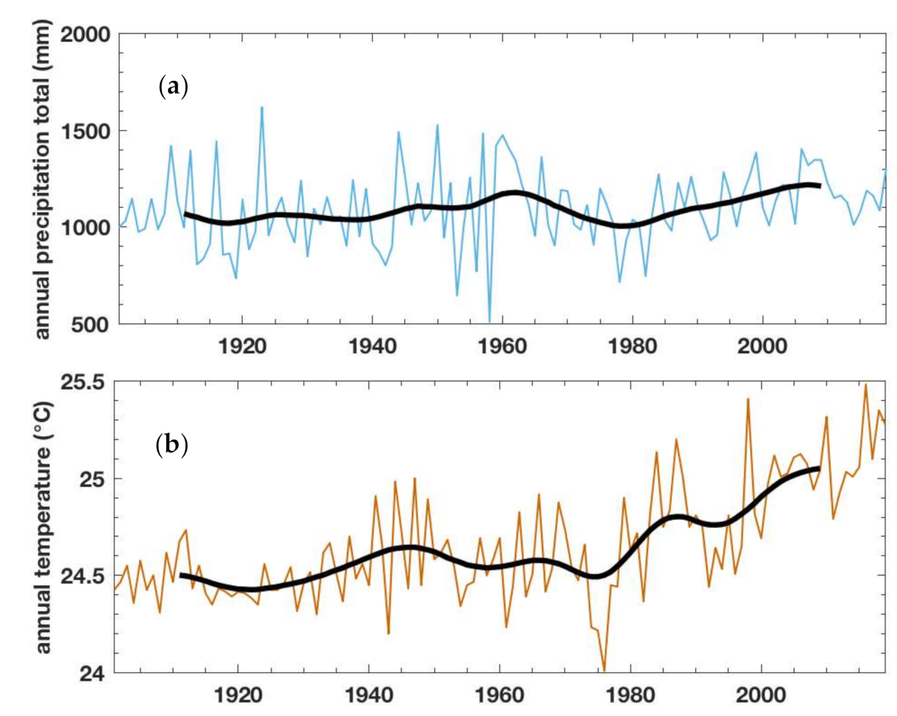
The present research was conducted in the Luki Biosphere Reserve, one of the protected areas in the Democratic Republic of Congo (Figure 1). Luki extends over an area of about 32,000 hectares and is located in the southwest part of the country, in the Kongo central province. The annual average rainfall is 1095.66 mm (Figure 2), mostly falling between October and May, with a marked dry season between May and September. The annual average temperature is 24.65 °C. The main vegetation types are tropical forests. The relatively high precipitation in the region allows the local communities to resort to year-round agricultural activities to support their families.
A large stretch of the national road crosses the Luki Reserve from Manterne to Kinzao-Mvuete and is a compulsory passage for vehicles. This partly explains the cause of the rapid growth of the villages on this route. It is worth noting that many illegal operators within the reserve live in these villages, compromising the sustainability of its natural resources.

2.2. Image Classification and Accuracy Assessment

Remotely sensed data (Landsat images and a digital elevation model with a spatial resolution of 30 m) were freely downloaded from http://glovis.usgs.gov/ and https://code.earthengine.google.com websites. From Google Earth Engine, Landsat images of the years 1987, 2002, 2017 and 2020 were downloaded. Also, the digital elevation model for the year 2000 was downloaded. In 2021, field data (500 observations per LUC category) were collected using a GPS receiver to provide a better understanding of different LUC categories in the study area.
Table 1 provides the description of the Landsat images used in the present research. Landsat images of the years 1987, 2002, 2017, and 2020 were radiometrically and atmospherically corrected using the FLAASH method. The landscape of the study area was then classified into five LUC types, including primary forest, savannah, fallow land and fields, secondary forest, and built-up area. The training and testing data of each year were created based on the field data collected for each LUC type in 2020 and the Google Earth images. Supervised classification was performed on the four images using the maximum likelihood algorithm. The maximum likelihood offers better classification results in the field of LUC study [42]. The accuracy assessment for the 1987, 2002, 2017, and 2020 maps was achieved using the Kappa statistic [43,44,45]. For all image processing, ENVI 5.3, QGIS, and ArcGIS were used.

2.3. MLPNN_Markov Chain Model for LUC Change Prediction

2.3.1. MLP Neural Network Model

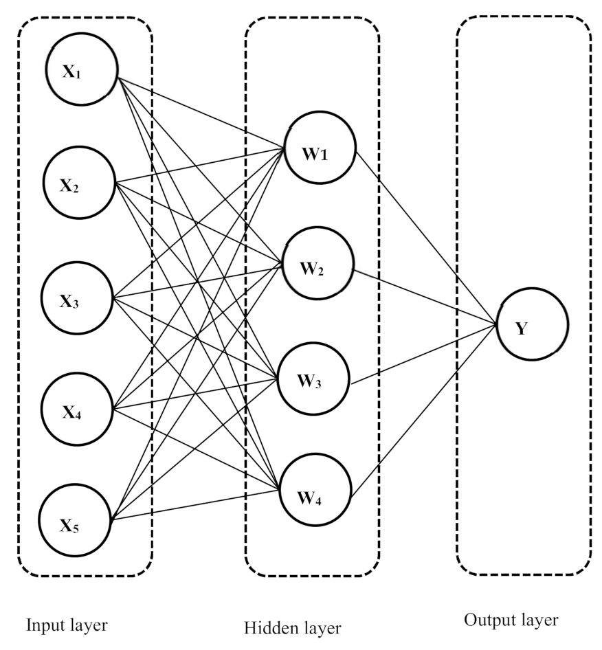
In recent decades, a number of studies have revealed the capability of the Artificial Neural Network algorithm in calibrating the LUC change modeling to predict its future trends [46,47,48,49]. The Artificial Neural Network algorithm was created by imitating the nervous system of the human being [50]. The present study used the Artificial Neural Network called multilayer perceptron neural network [51]. In the MLPNN algorithm, neurons or nodes are interconnected to create a complex neural network that is made up of three layers including an input layer, one or several hidden layers, and one output layer [52], as shown in Figure 3. Moreover, this model is made up of two types of input variables: the LUC images as dependent variables and the drivers of LUC change as independent variables. Each neuron in the input layer receives one of the input variables to produce an output value to the next layer. In that way, the input variables behave as signals that go through the layers in the MLPNN and finally produce output values. The mathematical formulation of the weighting process of the nodes in the input layers is presented below:
n e t j = i j o i .
i j represents the weights between node i and j. o i represents the output resulting from the node i. The mathematical computation of the output from a given node j is presented as follows [52]:
o i = f n e t i .
In the above formula, the nonlinear sigmoid function (f) is supposed to be applied on the weighted sum before the signal goes to the next layer. Nevertheless, in order to perform the correction of connection weights, the following formula is used [53]:
Δ j i   ( n + 1 ) =   ( δ j o i ) + α   Δ j i ( n ) .
ἠ represents the learning rate parameter; δj represents an index of the rate of change of the error; and α represents the momentum parameter.
Meanwhile, the performance of the neural network is affected by some other factors [52], including the number of nodes, number of training samples, number of iterations and the learning rate. Generally, the training accuracy is influenced by the sample size and iteration number. In fact, a small number of training samples may not represent the pattern of each class, while a great number of training samples may result in an overlap. Additionally, very few or too many iterations can lead to poor generalization of the model [53]. Indeed, the model runs with a number of iterations until the minimization of network errors [52]. The objective of performing the network training is to provide appropriate weights in order to perform the classification of unknown pixels [53]. The error rate is computed following the formula of the Root Mean Square (RMS) Error [54]:
R M S = e i N 2 = t i a i 2 N .
N represents the number of elements; i represents the index for elements; ei represents the error of the ith element; ti represents the target value (measured) for the ith element; and ai represents the calculated value for the ith element.
Finally, to better represent the training data, the neural network requires a more significant number of nodes in the hidden layer [52]. The mathematical expression to compute the number of nodes in the hidden layer is presented as follows [53]:
N h   = I N T   N i × N o .
Nh represents the number of hidden nodes; Ni represents the number of input nodes; No represents the number of output nodes.

2.3.2. Markov Chain Analysis

Markov chain techniques have been successfully applied in predicting LUC change. This model essentially examines the trend of transition probability of LUC classes in a given landscape over the specified number of time units. In this model, the LUC change can be described as a set of alternative states over time. This assumes that only the system state at time t can be used to determine its state at a given time (t + 1). In the present study, the Markov chain analysis was performed for the period between 1987 and 2002 to produce the transition probability matrix [56]. These matrices provide the transition probabilities for all LUC categories over the specified time and were used to predict the LUC map of 2017. The Markov chain analysis can be described using the following mathematical expression [57,58]:
S ( t ,   t + 1 ) = P i j   × S t   + 1 .
S(t) and S(t+1) represent the state of the system at time t and t + 1, respectively. P i j represents the transition probability matrix standing for the probability of the LUC class to transition from the state i to the state j, from the time t to the time t + 1. P i j   is mathematically computed using the following expression [59,60]:
P i j = P 11 P 12 P 13 P 1 n P 21 P 22 P 23 P 2 n P 31 P 32 P 33 P 3 n P n 1 P n 2 P n 3 P n n
( 0     P i j       1 )   and   j = 1 n P i j = 1 , i , j = 1 ,   2 , , n ) .
Pn represents the state probability of any time; n is the LUC type number; S is LUC status, t; t + 1 is the time point. Thus, any class with a low transition value will be expected to have a probability close to (0), while a high transition will have probabilities close to (1) [60].

2.3.3. Implementation of the MLPNN_Markov Modeling

During the transition potential modeling, the major LUC changes that occurred in the Luki Biosphere Reserve from 1987 to 2002 were identified and examined. This previous analysis was performed for the purpose of defining the transition categories. Consequently, the transition categories were well-defined, and the performance of the predictors was evaluated by means of the Cramer test [61]. In the present research, predictors with Cramer values >0.15 were used for predicting LUC change, as suggested by Hamdy et al. [62]. In fact, the range values of the Cramer test were between 0 and 1. Predictors with values close to 1 are reported to be more associated with the defined transition categories. Thus, their association with the defined transition categories are expected to be large. With respect to measuring the strength of association between predictors, the Cramer test is a nonparametric statistical analysis whose application does not relate to the variable distribution [63,64,65]. The Cramer’s V test is computed as follows:
V = x 2 n q 1 ,
x 2 = O E 2 2 .
V = Cramer’s index, n = sample size, q = smallest value in the rows and columns of the LUC image, O = observed frequency for a class, and E = expected frequency in the corresponding class.
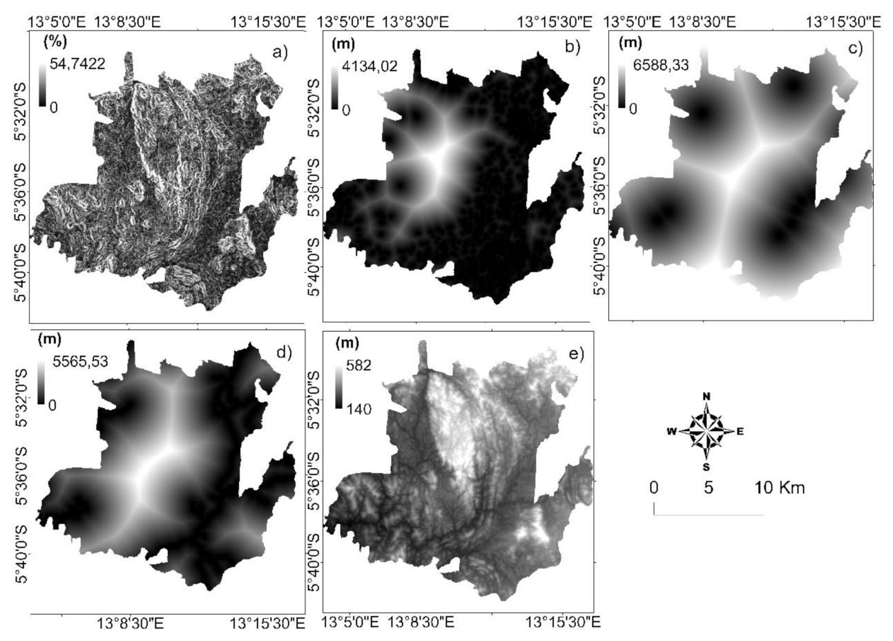
Predictors such as slope, altitude, distance from roads, distance from villages, and economic indicators have often been used for the purpose of predicting LUC change [1,30,65,66,67]. Thus, on the basis of the LUC change that occurred in the Luki Biosphere Reserve and the existing literature, five predictors were selected for the MLPNN_Markov modeling. These included the following variables: Distance from roads, distance from villages, distance from farmland, slope, and altitude (Figure 4). A digital elevation model was downloaded from the USGS website, and from this raster the slope raster was computed. Distance from roads and villages was computed by using the proximity tool in QGIS software. The vector data of roads and villages were converted to a raster file, then we calculated the distance of each pixel based on the road and village pixel. As for distance from existing farmlands, pixels of farmland for the corresponding period of prediction were extracted. The distance raster from farmland was then computed using the proximity tool in QGIS software.
After performing the Cramer’s V test, the MLPNN model was trained to compute the probabilities for each cell to transition from one type of LUC class to another from the year 1987 to 2002. Therefore, to improve the model performance, it is usually required to customize some parameters. In this case, the number of iterations was set to 10,000. The maximum sample size was customized based on the minimum number of pixels that was expected to transition from the initial date (1987) to the final date (2002). Afterwards, the learning rate, momentum, and hidden layers were customized by their default values. A given weight was then attributed to each major transition. The training process then started by dividing the sample data into validation and training, and then analyses on the accuracy of validation and training data. Finally, the training process was completed when the best accuracy was reached.
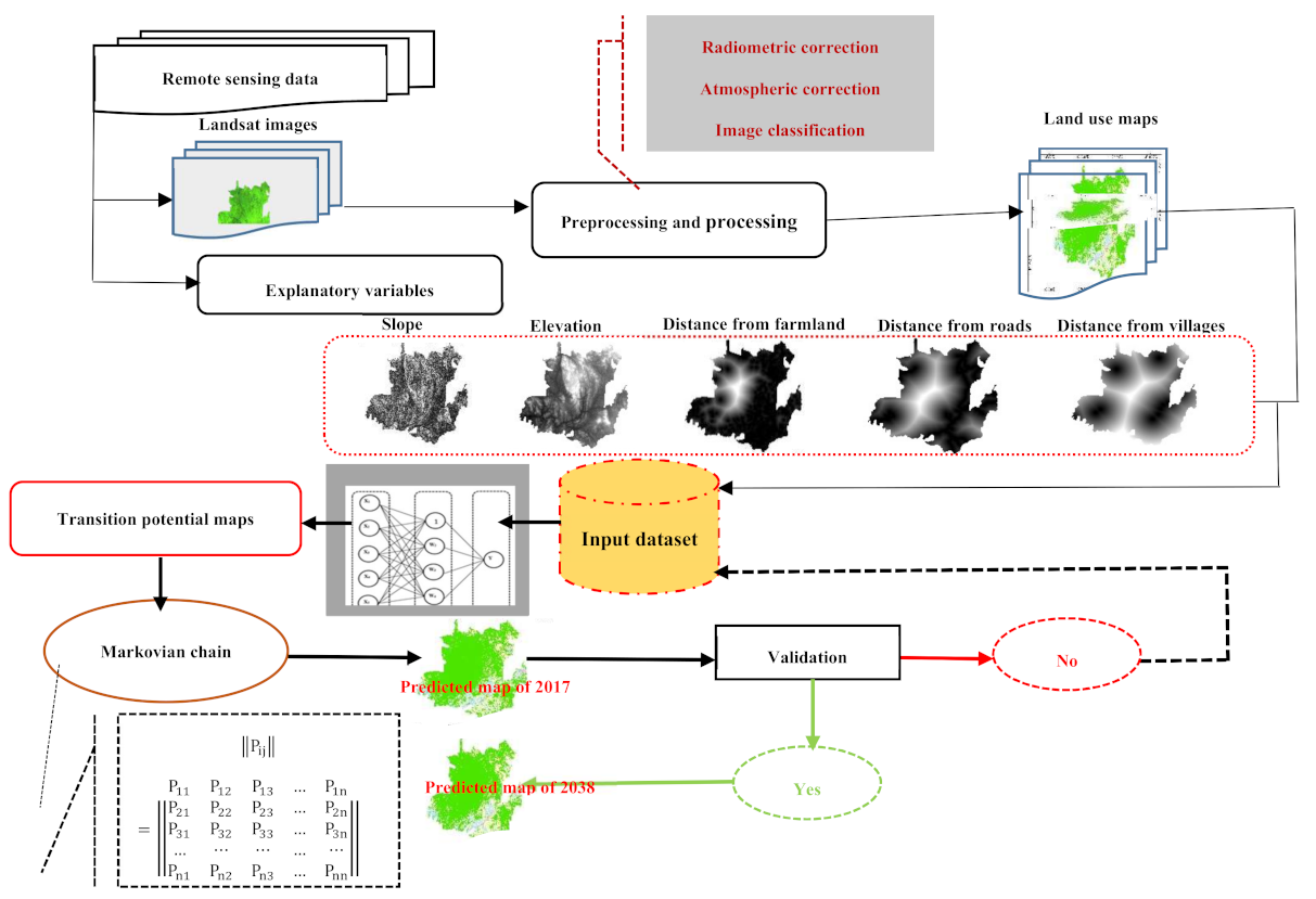
After the MLPNN model was finished, each transition contained the appropriate weight. These weights were incorporated in the Markov transition matrix for future prediction. Finally, the 2017 and 2038 maps were predicted using the transition potential maps derived from the MLPNN model and the Markov chain analysis. The workflow of the training and simulation process is illustrated in Figure 5.

2.3.4. Variables Selection

Based on the Cramer’s V test, the selection process of variables was performed. Table 2 shows the results related to the test of the driver variables, provided by the Cramer’s V test for the prediction of LUC change in the Luki Biosphere Reserve. Since their Cramer values were greater than 0.15, all the variables were used in the present study. These results revealed that all the explanatory variables had an influence on the LUC change process in the Luki Reserve, even though the elevation, distance from roads, and distance from existing fallow land and fields were revealed to be the most important. In general, areas close to existing fallow land and roads and with a high elevation were expected to experience more significant changes. Additionally, most areas close to villages were expected to experience a change in the region.

2.3.5. Model Validation

In this study, the validation process used the Pontius et al. [68] method. Here, the actual map of time 1 and time 2, and the predicted map of time 2 were used to generate the validation result, notably the agreement and disagreement component [69]. The agreement component was composed of two parts, i.e., correct rejection (persistence simulated correctly) and hits (change simulated correctly). The disagreement component was made up of three parts including misses (change predicted as persistence), false alarms (persistence predicted as change), and wrong hits (change predicted as a change to the wrong category). Thus, the reference map of 2002, the reference map of 2017, and the predicted maps of 2017 were used for that purpose.

2.4. Gradient Direction Analysis

Upscaling methods are widely used in the field of landscape ecology and gradient direction analysis and have been found to be very useful in examining the trend direction of land use/land cover change over time [70]. Firstly, the method starts by drawing several concentric rings on urban areas following a well-defined interval. The urban area and all land use/land cover classes that are less impacted by human activity (forest, water body, etc.) should be completely covered by the extent of the largest concentric ring. The next step involves drawing 16 fans through the rays extended from the urban center at defined intervals of 22.5°. Thus, a set of segment zones is generated at the level of the intersection between the concentric rings and the fans. Finally, the land use/land cover class with the largest proportion in each segment is selected to represent that segment.

2.5. Landscape Metrics Analysis

Landscape metrics analysis has been widely applied in the field of landscape ecology to quantify changes that may have occurred over time. Landscape structure analysis based on numerous metrics has been commonly used to examine spatiotemporal change in various land use/land cover classes. These changes can be examined and quantified following numerous landscape metrics related to the number, size, shape, and other parameters of the landscape that can be obtained from remote sensing data [71,72].
This study used four landscape metrics (Table 3), notably the Landscape Division Index (DIVISION), Patch Cohesion Index (COHESION), Aggregation index (AI), and Contagion index (CONTAG), to examine the spatial structure of the landscape [70]. Generally, the DIVISION and COHESION indices are used to measure the connectivity of the landscape habitat. The COHESION index ranges between 0 and 100. The null value is observed for the highly subdivided landscape and is physically less connected. The DIVISION varies between 0 and 1. The zero value is observed for the homogeneous landscape (landscape with a single patch), while the value of 1 is observed when the focal patch type consists of a single small patch, one cell in area. The aggregation index provides a measure of the specific class and is ranged between 0 and 100. The value of the index reaches 100 for a landscape whose focal patch type is maximally aggregated into a single compact patch. When the different types of land use are aggregated and geographically self-connected, they are characterized by high values of COHESION and AI indices. On the other hand, landscapes with land use types disconnected from each other are characterized by high values of the division index. CONTAG measures both the interspersion and the dispersion of patches at the landscape level. CONTAG values range from 0 to 100. The null values are observed in the landscape where patch types are characterized by minimum disaggregation, whereas it reaches 100 in the case of maximum aggregation. The FRAGSTATS software (version 4.2) as well as the landscape ecology plugin from QGIS [73], were used to carry out these quantitative analyses.

3. Results

3.1. Land Use/Land Cover Change of the Luki Biosphere Reserve

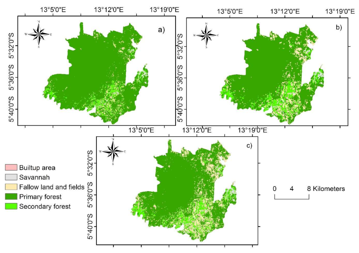
The past patterns (1987–2020) of the land use/land cover change were examined using Landsat images and the change detection technique. The overall classification accuracy was more than 80% for 1987, 2002, 2017, and 2020 classified images (Table 4). The landscape of the Luki Biosphere Reserve was classified into different land use/land cover classes including primary forest, secondary forest, fallow land and fields, savannah and built-up area (Table 5 and Figure 6). Primary forest remained the dominant class of the landscape since it was the major class. The class declined from approximately 87.59, 78.29 to 72.02% of the total area of Luki in 1987, 2002 and 2020, respectively. During the last four decades, primary forest lost 4811.93 hectares.
However, other land use/land cover classes experienced positive change from 1987 to 2020, except for savannah, which underwent negative change from 2002 to 2020. Fallow land and fields, secondary forest, savannah, and built-up area increased by 3852.12, 1150.36, 79.35, and 67.63 hectares, respectively. Secondary forest, built-up, and fallow land and fields quickly increased from 1981 to 2021, although most of the newly increased land use/land cover class was fallow land and fields.

3.2. Transition among Land Use/Land Cover Types from 1987 to 2038

The transition matrix (Table 6) provides the comprehensive direction change of different land use/land cover classes of the Luki Biosphere Reserve over the study period. From 1987 to 2020, the greatest loss of area was observed in the primary forest class. Additionally, the largest area of primary forest was converted into fallow land and fields, followed by secondary forest, savannah, and built-up area. Indeed, more than 13.26% of primary forests was converted into fallow land and fields due to the expansion of agricultural activities in the reserve. Further, the fallow land and field class recorded the largest areal gain, mainly converted from primary forest, secondary forests (7.8%), savannah (1.5%), and built-up area (0.8%). However, of the primary forest converted into fallow land and fields, 4% naturally evolved into secondary forest in the absence of human activities. Moreover, the overexploitation of primary forest areas over a long period led to their conversion into savannah. From 1987 to 2038, the highest amount of change is still expected to be observed converting primary forest to fallow land and fields; it will be even greater (16%) than that of the period between 1987 and 2020. Over this period, 3.1, 0.2, and 0.09% of the primary forest area will be converted into secondary forest, savannah, and built-up area, respectively. However, fallow land and fields will continue to increase in area coverage, 23.9, 29.7, and 7.1% of the increase are attributed to conversion from secondary forests, savannah, and built-up areas, respectively.

3.3. Land Use/Land Cover Change at Different Zonal Levels of the Luki Biosphere Zone

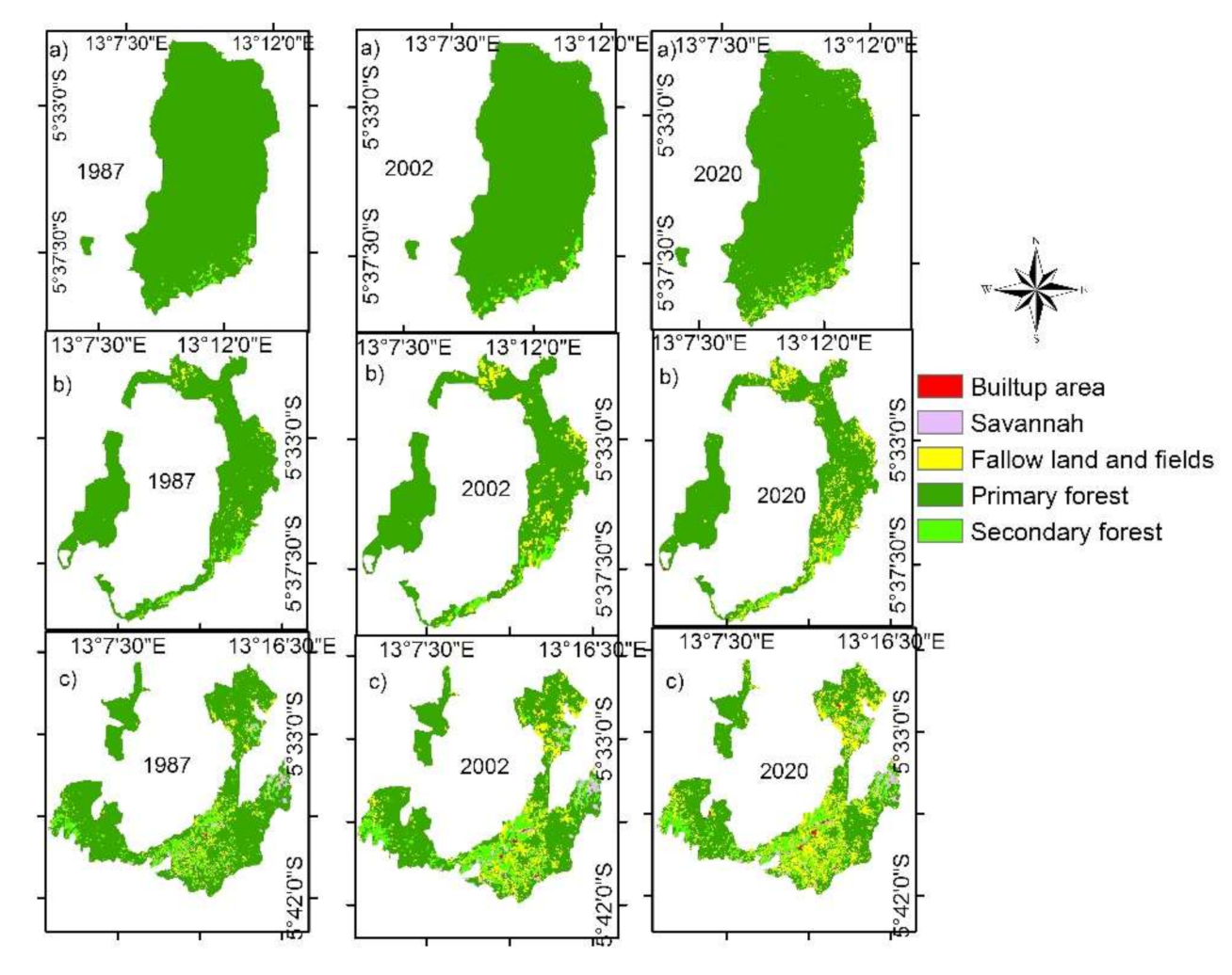
The landscape change in different zones of the Luki Biosphere Reserve is presented in Table 7, Table 8 and Table 9. The spatial pattern of change in each zone is also illustrated in Figure 7.
At the Core zone level, from 1987 to 2020 the primary forests lost 287.5 hectares while the fallow land and fields and secondary forest gained 194.5 and 93 hectares, respectively. This could be due to the illegal activities within this zone, including agricultural practices by the local communities, cutting timber for handcrafting, and charcoal for commercial use. With respect to the Buffer zone, a loss of 818.93 hectares of primary forests and 104.54 hectares of secondary forests was revealed. This could have resulted from the slash-and-burn agriculture practiced in this area. Thus, the fallow land and field class gained 704.73 hectares. Savannah and built-up areas also experienced an increase of 6.92 and 2.79 hectares, respectively. The Transition zone underwent dramatic changes in turn. In fact, from 1987 to 2020, the primary forest experienced a reduction of 4040.55 hectares. The secondary forests in turn gained 948.7 hectares. Several hectares of forests converted into agricultural areas were found to have evolved into secondary forests. Agricultural areas increased to around 2954.63 hectares. The savannah class recorded a gain of 72.39 hectares from 1987 to 2020. On the other hand, from 2002 to 2020, a decrease of 62.83 hectares was observed due to the practices of defending savannas in certain areas of the reserve.

3.4. Landscape Metrics Analysis at the Luki Biosphere Reserve

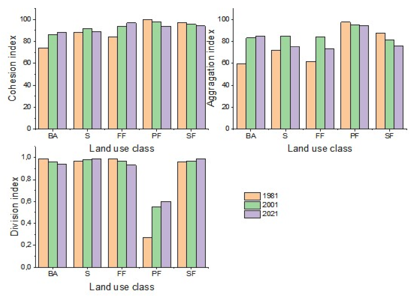
In the present study, four landscape metrics, including patch cohesion index, contagion index, aggregation index and landscape division, were computed to examine landscape structure and change of different land use/land cover classes (Figure 8). The primary forest was the dominant land use/land cover class in the Luki Biosphere Reserve landscape, and the change induced in this class was also closely related to eco-environmental issues such as deforestation, land degradation, biodiversity lost, wildlife habitats destruction, and wildlife migration. From 1987 to 2020, there was an increase in the landscape division metric within the primary forest (starting from 0.27 to 0.63), while the patch cohesion index decreased from 99.9 to 93.8. In addition, the aggregation index decreased from 97.6 to 94.5. This contributed to the fragmentation and the reduction of the self-connectivity inside the primary forest. A similar decreasing trend in the patch cohesion index was observed in the secondary forest from 2002 to 2020, with a slight increase of the division metrics. The fallow land and fields and the built-up area experienced an opposite trend for both division and cohesion metrics, when compared with the primary forest. In fact, these two land use/land cover classes experienced an increasing trend in the cohesion index and a decreasing trend in the division index, indicating that they gradually expanded outwards from 1987 to 2020. As for the savannah class, a slight increase in division index was observed. With respect to the aggregation and cohesion indices, the savannah class experienced an increasing trend from 1987 to 2002, while a decreasing trend was observed from 2002 to 2020.

3.5. Impact of Village Expansion on Land Use/Land Cover Change

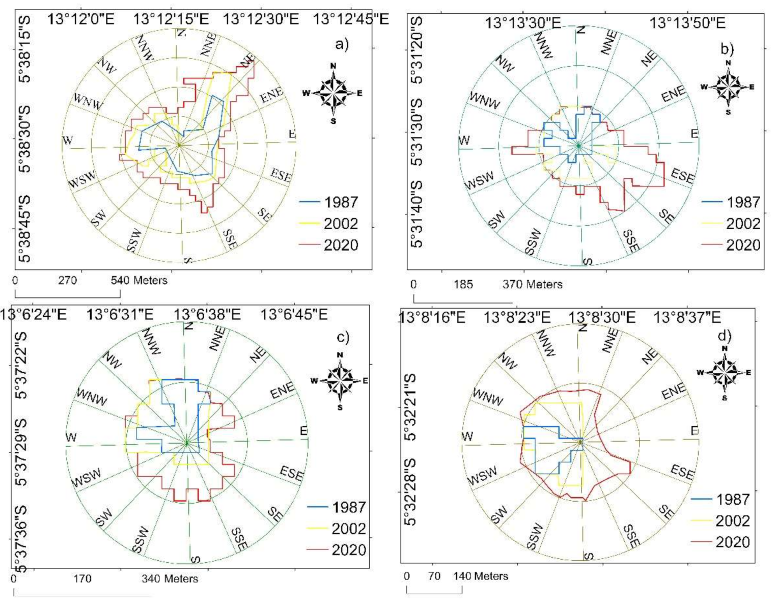
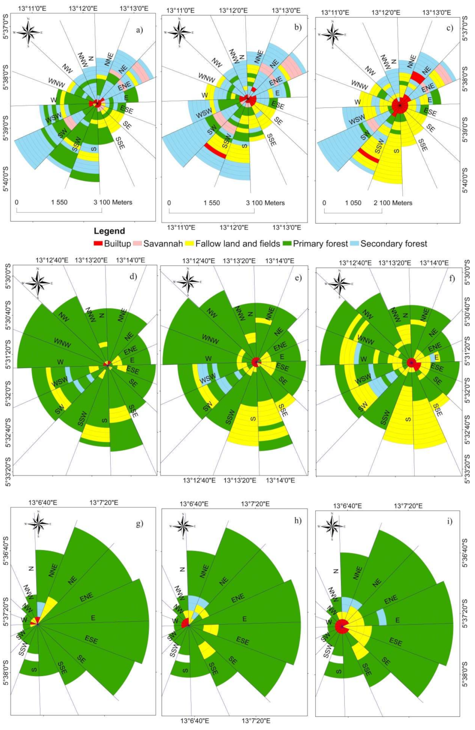
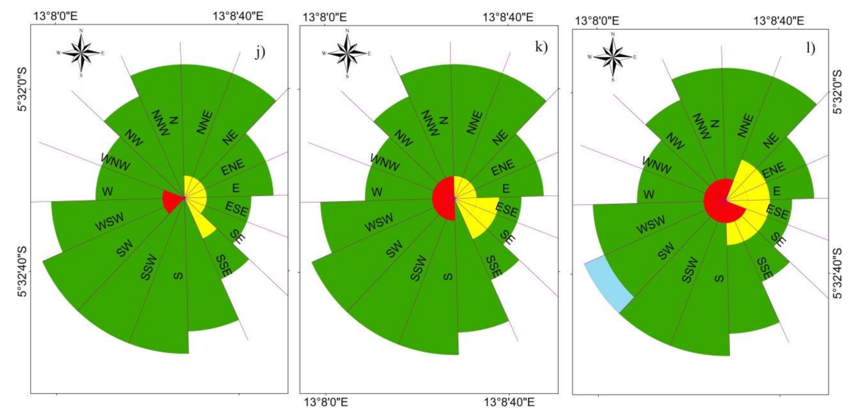
The gradient direction analysis was used for the purposes of visualizing and understanding the direction of land use/land cover change over the time. This was in response to population growth and village expansion (Figure 9 and Figure 10) from the center of the four enclaves (four villages legally established in the reserve), including Tsumba-Kituti, Kiobo, Kisavu and Kibuya. In 1987, land use/land cover classes of Tsumba-Kituti comprised primary forest, secondary forest, savannah, fallow land and fields, and built-up area. The region consisted of several villages whose expansion dramatically contributed to observed changes in the landscape. The center of the region was dominated by the settlements, while the southern part showed a pronounced decrease in the primary forest. The secondary forest experienced a slight decrease across all the regions, while the southern region recorded a high decrease compared to other regions. Fallow land and fields increased in all directions. As for Kisavu village, in 1987 the landscape was dominated by primary forest. However, the expansion of the village induced major changes in the landscape. Over the past 40 years, a huge amount of primary forest was converted into fallow land and fields and secondary forest. Most of these changes were observed in the southern and eastern part of the villages where local communities established farm lands for crop cultivation. For the Kiobo village, primary forest was converted into fallow land and fields, particularly in the southern part of the village. Additionally, some areas of primary forest in the northern part of the village were slightly converted into secondary forest due to the artisanal wood logging that often leads to the degradation of primary forest. Finally, the Kibuya region experienced a slight increase in fallow land and fields in the eastern part due to the expansion of croplands.

4. Discussion

4.1. Land Use Change of the Luki Biosphere Reserve

Natural ecosystems are of crucial importance for the survival of humanity as they provide ecosystem services, including air purification, climate regulation, food provision, regulation of environmental problems, and conservation of water resources. Population growth and expansion of urban areas are the bases for the transformation of natural landscapes through the conversion of natural ecosystems (forest, savannah, water, wetlands, etc.) into built-up areas, crop and degraded areas. Several studies have shown that urban expansion and population growth are at the root of the problems associated with heat islands [80,81,82], the increase in carbon emissions, and the loss of carbon [83]. In the Democratic Republic of Congo, several studies have revealed that population growth and urban expansion increases the proliferation of cultivation areas as well as the degradation of natural ecosystems [23,84,85,86,87]. Indeed, many natural land use types have been converted into crop, plantation, and degraded areas due to economic benefits. The loss of natural ecosystems and the intensification of cultivation areas or urban expansion have been the bases of several environmental problems [80,88,89].
In the Luki Biosphere Reserve, most of the villages were developed along the first national road, which connects the two main cities in the region to the city province of Kinshasa, and whose demand for natural resources as well as crop products has been increasing. This continues to increase the risks to the natural resources within the reserve, including deforestation, degradation, and disappearance of species of fauna.
The fragmentation of natural landscapes is another problem caused by urbanization and population growth [75,90,91]. According to Gkyer [92], landscape metrics analysis can help natural resources managers to better comprehend changes that have occurred in the landscape. Numerous landscape metrics, particularly the indices of division, aggregation and cohesion, can reveal the presence of fragmentation of natural ecosystems caused by human activities [92]. Indeed, the landscape division metric can be evaluated over time, and its increase can inform on the fragmentation of the landscape. The patch cohesion index and the aggregation index can also inform on the fragmentation of the landscape when their values decrease. Thus, in the Luki Biosphere Reserve, from 1987 to 2020 the observed increase in the landscape division metric within the primary forest (from 0.27 to 0.63), and the decreases in the patch cohesion index (from 99.9 to 93.8) and the aggregation index (97.6 to 94.5) indicated the fragmentation of the primary forest class leading to the reduction of its self-connectivity. As for the secondary forest class, we observed a decrease trend in the patch cohesion index from 2002 to 2020, while the division metrics slightly increased. In fact, due to human activities, primary and secondary forest have been prone to unsustainable exploitation leading to their fragmentation over the years. An opposite trend was observed in the fallow land and fields and the built-up area, for both division and cohesion metrics, when compared with the primary forest. Indeed, these two classes have experienced an expansion over the years leading to the increase in the cohesion metrics and the decrease in the division metrics.
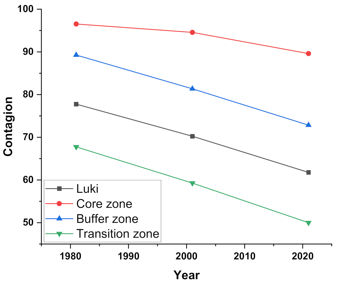
As shown in Figure 11, the CONTAG index demonstrated the fragmentation of land not only in the entire reserve but also at the zonal level. A high CONTAG value means that the dominant land use patches are well connected within a landscape, while low values indicate that the landscape is more fragmented. CONTAG values decreased from the central area to the transition area. However, landscape fragmentation was observed in all zones of the reserve. The Core zone was characterized by the highest CONTAG values, but they steadily decreased from 1987 to 2020. This means that the landscape of the Core zone was less fragmented compared to the other zones. With the most complex land use/land cover types, the Transition zone’s landscape was the most fragmented. From 1987 to 2020, there was an increasing trend of land fragmentation in all zones, as CONTAG continuously decreased in all zones. Fragmentation of land can lead to problems related to land and wildlife management. Fragmentation reduces ecological corridors, endangering animal biodiversity. In Bangkok, the fragmentation of green spaces was found to reduce the density of pollinators, even when floral resources were abundant [93]. Similarly, Chaiyarat et al. [94] reported a decline in bird diversity following the fragmentation of green spaces.

4.2. Prediction of Land Use/Land Cover Change

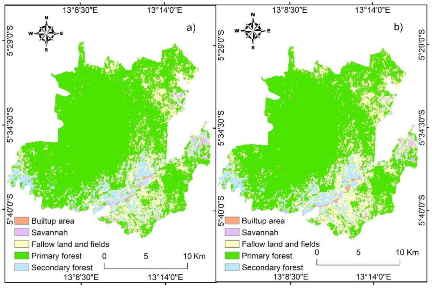
The present research examined LUC change in the Luki Biosphere Reserve over the past 33 years (from 1987 to 2020) with an aim of predicting future LUC changes for the year 2038. Five explanatory variables were used for this purpose, including distance from roads, distance from villages, distance from existing farmland, slope, and elevation [93]. Prediction of the future LUC was obtained by means of the land change modeler plugin implemented in IDRISI software. Thus, based on the LUC change between 1987 and 2002, the transition potential maps were created using the MLPNN algorithm. Afterwards, a simulated map of 2017 was produced using the Markovian chain model. The CROSSTAB module in IDRISI was then used for model validation. Noteworthy was the validation process used in the Pontius et al. [68] method. The results obtained revealed a low percentage of disagreement components (3.6%) and a high percentage of agreement components (96.4%) (Table 10). Since the validation results provided a high accuracy, the transition potential maps between 2002 and 2017 were then used to predict the 2038 land use/land cover map (Figure 12) following the same approach. The time interval used to predict the 2038 map was 15 years.
Overall, in 2038 there will still be a decrease in primary forest and savannah of around 899.43 and 223.12 hectares, respectively. The secondary forest will also experience a decrease, losing around 518.88 hectares from 2020 to 2038 due to its proximity to roads and villages, which will lead to its conversion to fallow land and fields. However, built-up area and fallow land and fields will still experience a great expansion by gaining 65.07 and 1576.41 hectares, respectively. The decrease in primary forest can be attributed to the development of unsustainable agriculture, wood energy, expansion of built-up area, and artisanal wood logging. Although savannah decrease is attributed to the expansion of farmland and built-up area, it was noticed that the effort of protecting savannah led to the conversion of this land use/land cover class to forest land.

5. Conclusions

Since 1987, the Luki Biosphere Reserve and all its zones, including the Core zone, Buffer zone and Transition zone, have undergone dramatic land use/land cover change. The primary forest land decreased throughout the reserve and across all the zones. Secondary forest, savannah, built-up area, and fallow land and fields increased from 1987 to 2020. The Transition zone had the highest land use/land cover change intensity, followed by the Buffer zone and Core zone. The prediction results indicated that there will still be a great decrease in primary forest, while other land use/land cover classes will still face a great expansion, except the secondary forest, which will experience a slight decrease from 2020 to 2038. With respect to landscape analysis, most villages showed clear spatial orientations in the process of village expansion. A strengthening of the connectivity of built-up areas and fallow land was observed throughout the reserve, as well as a phenomenon of fragmentation and disaggregation of other classes of land use outside the built-up area (such as primary forest, secondary forest, and savannah). Over the past few decades, most natural land use types were transformed and replaced by newly grown built-up areas, fallow land and fields. Environmental issues such as environmental degradation, loss of biodiversity, and soil erosion can arise from the loss of different natural land use/land cover classes in the Luki Biosphere Reserve. In addition to this, the fragmentation of the landscape can negatively affect the future of biodiversity in the reserve. Therefore, future studies on the environmental impacts driven by land use/land cover change in the Luki Biosphere Reserve should be initiated to provide reliable information for decision makers for sustainable forest management. Additionally, studies on the dependency of local communities on forest resources should be undertaken in different villages and their surroundings.

Author Contributions

Conceptualization, method development and writing: O.O.M., F.W., Y.Y., K.S.K.; visualization and data processing: O.O.M. and C.C.; investigation and resources: O.O.M. All authors have read and agreed to the published version of the manuscript.

Funding

This study was supported by The Fundamental Research Funds for the Central Universities (2572019CP12).

Institutional Review Board Statement

Not applicable.

Informed Consent Statement

Not applicable.

Data Availability Statement

Not applicable.

Acknowledgments

We thank all our research group members for their continuous supports.

Conflicts of Interest

The authors declare no conflict of interest.

References

  1. Han, H.; Yang, C.; Song, J. Scenario Simulation and the Prediction of Land Use and Land Cover Change in Beijing China. Sustainability 2015, 7, 4260–4279. [Google Scholar] [CrossRef] [Green Version]
  2. Rawat, J.S.; Kumar, M. Monitoring land use/cover change using remote sensing and GIS techniques: A case study of Hawalbagh block, district Almora, Uttarakhand, India. Egypt. J. Remote Sens. Space Sci. 2015, 18, 77–84. [Google Scholar] [CrossRef] [Green Version]
  3. McConnell, W.J. Land Change: The Merger of Land Cover and Land use Dynamics. In International Encyclopedia of the Social & Behavioral Sciences, 2nd ed.; Elsevier: Oxford, UK, 2015; pp. 220–223. [Google Scholar]
  4. Lambin, E. Land Cover Assessment and Monitoring. In Encyclopedia of Analytical Chemistry; John Wiley & Sons, Ltd.: Hoboken, NJ, USA, 2006. [Google Scholar] [CrossRef]
  5. Hyandye, C.; Martz, L.W. A Markovian and cellular automata land-use change predictive model of the Usangu Catchment. Int. J. Remote Sens. 2016, 38, 64–81. [Google Scholar] [CrossRef]
  6. Galicia, L.; Garcia-Romero, A. Land use and land cover change in highland temperate forests in the Izta-Popo National Park, central Mexico. Mt. Res. Dev. 2007, 27, 48–57. [Google Scholar] [CrossRef]
  7. Fox, J.; Vogler, J.B. Land-use and land-cover change in montane mainland Southeast Asia. Environ. Manag. 2005, 36, 394–403. [Google Scholar] [CrossRef]
  8. Ouedraogo, I.; Tigabu, M.; Savadogo, P.; Compaoré, H.; Odén, P.C.; Ouadba, J.M. Land cover change and its relation with population dynamics in Burkina Faso, West Africa. Land Degrad. Dev. 2010, 21, 453–462. [Google Scholar] [CrossRef]
  9. Ernst, C.; Verhegghen, A.; Mayaux, P.; Hansen, M.; Defourny, P. Cartographie du couvert forestier et des changements du couvert forestier en Afrique centrale. In Les Forets du Bassin du Congo—Etat des Forets 2010; De Wasseige, C., De Marcken, P., Bayol, N., Hiol Hiol, F., Mayaux, P., Desclee, B., Billand, A., Nasi., R., Eds.; Office des Publications de l’Union Europeenne: Luxembourg, 2012; pp. 23–42. [Google Scholar] [CrossRef]
  10. Devers, D.; Van de Weghe, J.P. (Eds.) Les Forêts du Bassin du Congo. État des forêts 2006. Partenariat pour les forêts du Bassin du Congo; United States Agency for International Development: Washington, DC, USA, 2007; 256p. Available online: http://carpe.umd.edu/Documents/2006/LES_FORETS_DU_BASSIN_DU_CONGO_Etat_des_Forets_2006.pdf (accessed on 8 May 2021).
  11. Gillet, P.; Vermeulen, C.; Feintrenie, L.; Dessard, H.; Garcia, C. Quelles sont les causes de la deforestation dans le bassin du Congo? Synthese bibliographique et etudes de cas. BASE 2016, 20, 183–194. [Google Scholar]
  12. Potapov, P.V.; Turubanova, S.V.; Hansen, M.C.; Adusei, B.; Broich, M.; Altstatt, A.; Mane, L.; Justice, C.O. Quantifying forest cover loss in Democratic Republic of the Congo, 2000–2010, with Landsat ETM+ data. Remote Sens. Environ. 2012, 122, 106–116. [Google Scholar] [CrossRef]
  13. Duveiller, G.; Defourny, P.; Desclee, B.; Mayaux, P. Deforestation in Central Africa: Estimates at regional, national and landscape levels by advanced processing of systematically- distributed Landsat extracts. Remote Sens. Environ. 2008, 112, 1969–1981. [Google Scholar] [CrossRef]
  14. Muyaya, K.B.; Rudant, J.P.; Lumbuenamo, R.; Beland, M.; Riera, B. Dynamique spatiale du domaine de chasse et reserve de Bombo Lumene entre 2000 et 2015 par imagerie satellitaire optique. Int. J. Innov. Appl. Stud. 2016, 2, 559–568. [Google Scholar]
  15. De Wasseige, C.; de Marcken, P.; Bayol, N.; Hiol, F.; Mayaux, P.; Desclee, B.; Billand, A.; Nasi, R. Les Forets du Bassin du Congo –Etat des Forets 2010; Office des publications de l’Union europeenne: Luxembourg, 2012; 276p. [Google Scholar]
  16. Molinario, G.; Hansen, M.C.; Potapov, P.V. Forest cover dynamics of shifting cultivation in the Democratic Republic of Congo: A remote sensing-based assessment for 2000–2010. Environ. Res. Lett. 2015, 10. [Google Scholar] [CrossRef]
  17. Pendje, G.; Mbaya, M. La réserve de Biosphère de Luki, Patrimoine Floristique et Faunique en Péril; UNESCO: Paris, France, 1992; 62p. [Google Scholar]
  18. Doumenge, C. La Conservation des Écosystèmes Forestiers du Zaïre; UICN: Gland, Switzerland, 1990; p. 242. [Google Scholar]
  19. Gata, D. Etudes des Impacts Humains, Estimation De Degré de Péril de la Biodiversité et Principes Directeurs pour une Gestion Durable des Ressources Disponibles; MAB: Kinshasa, Democratic Republic of the Congo, 1997; 37p. [Google Scholar]
  20. Nyange, N.M. Participation des communautés locales et gestion durable des forêts: Cas de la réserve de la biosphère de Luki en République Démocratique du Congo. Ph.D. Thesis, Université Laval Québec, Québec, QC, Canada, 2014; 227p. Available online: https://corpus.ulaval.ca/jspui/bitstream/20.500.11794/25349/1/30892.pdf (accessed on 2 May 2021).
  21. Cromley, R.; Hanink, D. Coupling land use allocation models with raster GIS. J. Geograph. Syst. 1999, 1, 137–153. [Google Scholar] [CrossRef]
  22. Sahebgharani, A. Multi-objective land use optimization through parallel particle swarm algorithm: Case study Baboldasht district of Isfahan, Iran. J. Urban Environ. Eng. 2016, 10, 42–49. [Google Scholar] [CrossRef]
  23. Opelele, O.M.; Fan, W.Y.; Yu, Y.; Kachaka, S.K. Analysis of land use/land cover change and its prediction in the mambasa sector, democratic republic of Congo. Appl. Ecol. Environ. Res. 2020, 18, 5627–5644. [Google Scholar] [CrossRef]
  24. Abdulrahman, A.I.; Ameen, S.A. Predicting Land use and land cover spatiotemporal changes utilizing CA-Markov model in Duhok district between 1999 and 2033. Acad. J. Nawroz Univ. 2020, 9, 71–80. [Google Scholar] [CrossRef]
  25. Mondal, B.; Das, D.N.; Bhatta, B. Integrating cellular automata and Markov techniques to generate urban development potential surface: A study on Kolkata agglomeration. Geocarto Int. 2017, 32, 401–419. [Google Scholar] [CrossRef]
  26. QuanLi, X.; Kun, Y.; GuiLin, W.; YuLian, Y. Agent-based modeling and simulations of land-use and land-cover change according to ant colony optimization: A case study of the Erhai Lake Basin, China. Nat. Hazards 2015, 75, 95–118. [Google Scholar] [CrossRef]
  27. Mishra, V.N.; Rai, P.K. A remote sensing aided multilayer perceptron-Markov chain analysis for land use and land cover change prediction in Patna district (Bihar), India. Arab. J. Geosci. 2016, 9. [Google Scholar] [CrossRef]
  28. Balzter, H. Markov chain models for vegetation dynamics. Ecol. Modell. 2000, 126, 139–154. [Google Scholar] [CrossRef] [Green Version]
  29. Mishra, V.N.; Rai, P.K.; Prasad, R.; Punia, M.; Nistor, M.M. Prediction of spatio-temporal land use/land cover dynamics in rapidly developing Varanasi district of Uttar Pradesh, India, using geospatial approach: A comparison of hybrid models. Appl. Geomat. 2018, 10, 257–276. [Google Scholar] [CrossRef]
  30. Feng, Y.; Liu, Y. A heuristic cellular automata approach for modelling urban land-use change based on simulated annealing. Int. J. Geogr. Inf. Sci. 2012, 27, 449–466. [Google Scholar] [CrossRef]
  31. National Research Council. Advancing Land Change Modeling: Opportunities and Research Requirements; The National Academies Press: Washington, DC, USA, 2014; ISBN 978-0-309-28833-0. [Google Scholar]
  32. Ansari, A.; Golabi, M.H. Prediction of spatial land use changes based on LCM in a GIS environment for Desert Wetlands—A case study: Meighan Wetland, Iran. Int. Soil Water Conserv. Res. 2019, 7, 64–70. [Google Scholar] [CrossRef]
  33. Mozumder, C.; Tripathi, N.K. Geospatial scenario based modelling of urban and agricultural intrusions in Ramsar wetland deepor beel in northeast India using a multilayer perceptron neural network. Int. J. Appl. Earth Obs. Geoinf. 2014, 32, 92–104. [Google Scholar] [CrossRef]
  34. Bhatti, S.S.; Tripathi, N.K.; Nitivattananon, V.; Rana, I.A.; Mozumder, C. A multi-scale modeling approach for simulating urbanization in a metropolitan region. Habitat Int. 2015, 50, 354–365. [Google Scholar] [CrossRef] [Green Version]
  35. Shoyama, K.; Matsui, T.; Hashimoto, S.; Kabaya, K.; Oono, A.; Saito, O. Development of land-use scenarios using vegetation inventories in Japan. Sustain. Sci. 2019, 14, 39–52. [Google Scholar] [CrossRef]
  36. Ye, B.; Bai, Z. Simulating land use/cover changes of Nenjiang County based on CA-Markov model. Comput. Comput. Technol. Agric. 2008, 1, 321–329. [Google Scholar] [CrossRef] [Green Version]
  37. Pontius, G.R.; Malanson, J. Comparison of the structure and accuracy of two land change models. Int. J. Geogr. Inf. Sci. 2005, 19, 243–265. [Google Scholar] [CrossRef]
  38. Parsamehr, K.; Gholamalifard, M.; Kooch, Y. Comparing three transition potential modeling for identifying suitable sites for REDD+ projects. Spat. Inf. Res. 2020, 28, 159–171. [Google Scholar] [CrossRef]
  39. Muller, M.R.; Middleton, J. A Markov model of land-use change dynamics in the Niagara Region, Ontario, Canada. Landsc. Ecol. 1994, 9, 151–157. [Google Scholar] [CrossRef]
  40. Sinha, P.; Kimar, L. Markov land cover change modeling using pairs of time-series satellite images. Photogramm. Eng. Remote Sens. 2013, 79, 1037–1051. [Google Scholar] [CrossRef]
  41. Harris, I.; Osborn, T.J.; Jones, P.; Lister, D.H. Version 4 of the CRU TS monthly high-resolution gridded multivariate climate dataset. Sci. Data 2020, 7, 109. [Google Scholar] [CrossRef] [Green Version]
  42. Vadrevu, K.P. Introduction to Remote Sensing. In The Photogrammetric Record, 5th ed.; Campbell, J.B., Wynne, R.H., Eds.; Guilford Press: New York, NY, USA, 2013. [Google Scholar]
  43. Keshtkar, H.; Voigt, W.; Alizadeh, E. Land-cover classification and analysis of change using machine learning classifiers and multi-temporal remote sensing imagery. Arab. J. Geosci. 2017, 10. [Google Scholar] [CrossRef]
  44. Pijanowski, B.C.; Pithadia, S.; Shellito, B.A. Calibrating a neural network-based urban change model for two metropolitan areas of the Upper Midwest of the United States. Int. J. Geogr. Inf. Sci. 2005, 19, 197–215. [Google Scholar] [CrossRef]
  45. Congalton, R.G.; Mead, R.A. A quantitative method to test for consistency and correctness in photo-interpretation. Photogramm. Eng. Remote Sens. 1983, 49, 69–74. [Google Scholar]
  46. Ju, W.; Lam, N. Urban land use classification: Applying texture analysis and artificial intelligence. Imaging Notes 2007, 22, 26–30. [Google Scholar] [CrossRef] [Green Version]
  47. Li, X.; Yeh, A.G.O. Neural-network-based cellular automata for simulating multiple land use changes using GIS. Int. J. Geogr. Inf. Sci. 2002, 16, 323–343. [Google Scholar] [CrossRef]
  48. Okwuashi, O.; Isong, M.; Eyo, E.; Eyoh, A.; Nwanekezie, O.; Olayinka, D.N.; Udoudo, D.O.; Ofem, B. GIS Cellular automata using artificial neural network for land use change simulation of Lagos, Nigeria. J. Geogr. Geol. 2012, 4. [Google Scholar] [CrossRef] [Green Version]
  49. Mahajan, Y.; Venkatachalam, P. Neural network based cellular automata model for dynamic spatial modeling in GIS. In Computational Science and Its Applications—ICCSA 2009; Gervasi, O., Taniar, D., Murgante, B., Laganà, A., Mun, Y., Eds.; Springer: Berlin/Heidelberg, Germany, 2009; pp. 341–352. [Google Scholar]
  50. Civco, D.L. Artificial neural networks for land-cover classification and mapping. Int. J. Geogr. Inf. Syst. 1993, 7, 173–186. [Google Scholar] [CrossRef]
  51. Haykin, S. Redes Neurais; Bookman: Porto Alegre, Brazil, 2001; p. 900. [Google Scholar]
  52. Atkinson, P.M.; Tatnall, A.R.L. Introduction neural networks in remote sensing. Int. J. Remote Sens. 1997, 18, 699–709. [Google Scholar] [CrossRef]
  53. Eastman, J.R. IDRISI Taiga Guide to GIS and Image Processing; Manual Version 16.02; Clark Labs: Worcester, MA, USA, 2009. [Google Scholar]
  54. Karul, C.; Soyupak, S. A comparison between neural network based and multiple regression models for chlorophyll-a estimation. In Ecological Informatics; Recknagel, F., Ed.; Springer: Berlin, Germany, 2006; pp. 309–323. [Google Scholar] [CrossRef]
  55. Yang, J.; Su, J.; Chen, F.; Xie, P.; Ge, Q. A local land-use competition cellular automata model and its application. ISPRS Int. J. Geo-Inf. 2016, 5, 106. [Google Scholar] [CrossRef] [Green Version]
  56. Mishra, V.N.; Rai, P.K.; Mohan, K. Prediction of land use changes based on land change modeler (LCM) using remote sensing: A case study of Muzaffarpur (Bihar), India. J. Geogr. Inst. Jovan Cvijic SASA 2014, 64, 111–127. [Google Scholar] [CrossRef]
  57. Yousheng, W.; Xinxiao, Y.; Kangning, H.; Qingyun, L.; Yousong, Z.; Siming, S. Dynamic simulation of land use change in Jihe watershed based on CA-Markov model. Trans. Chin. Soc. Agric. Eng. 2011, 27, 330–336. [Google Scholar] [CrossRef]
  58. Ma, C.; Zhang, G.Y.; Zhang, X.C.; Zhao, Y.J.; Li, H.Y. Application of Markov model in wetland change dynamics in Tianjin Coastal Area, China. Procedia Environ. Sci. 2012, 13, 252–262. [Google Scholar] [CrossRef] [Green Version]
  59. Sang, L.; Zhang, C.; Yang, J.; Zhu, D.; Yun, W. Simulation of land use spatial pattern of towns and villages based on CA–Markov model. Math. Comput. Model 2011, 54, 938–943. [Google Scholar] [CrossRef]
  60. Kumar, S.; Radhakrishnan, N.; Mathew, S. Land use change modelling using a Markov model and remote sensing. Geomat. Nat. Hazards Risk 2014, 5, 145–156. [Google Scholar] [CrossRef]
  61. Cramér, H. Methods of estimation. In Mathematical Methods of Statistics, 19th ed.; Princeton University Press: Princeton, NJ, USA, 1999; Chapter 33; pp. 497–506. [Google Scholar]
  62. Hamdy, O.; Zhao, S.; Salheen, M.A.; Eid, Y.Y. Analyses the driving forces for urban growth by using IDRISI Selva Models Abouelreesh—Aswan as a Case Study. Int. J. Eng. Technol. 2017, 9, 226–232. [Google Scholar] [CrossRef] [Green Version]
  63. Valdivieso, F.O.; Sendra, J.B. Application of GIS and remote sensing techniques in generation of land use scenarios for hydrological modeling. J. Hydrol. 2010, 395, 256–263. [Google Scholar] [CrossRef]
  64. Liebertrau, A.M. Measures of Association; Sage Publications: Newbury Park, CA, USA, 1983; Quantitative. [Google Scholar]
  65. Islam, K.; Rahman, M.F.; Jashimuddin, M. Modeling land use change using cellular automata and artificial neural network: The case of Chunati Wildlife Sanctuary, Bangladesh. Ecol. Indic. 2018, 88, 439–453. [Google Scholar] [CrossRef]
  66. Brown, D.G.; Goovaerts, P.; Burnicki, A.; Li, M.Y. Stochastic simulation of land cover change using geostatistics and generalized additive models. Photogramm. Eng. Remote Sens. 2002, 68, 1051–1061. [Google Scholar]
  67. Badoe, D.A.; Miller, E.J. Transportation–land-use interaction: Empirical findings in North America, and their implications for modeling. Transp. Res. Part D Transp. Environ. 2000, 5, 235–263. [Google Scholar] [CrossRef]
  68. Pontius, R.G.; Millones, M. Death to Kappa: Birth of quantity disagreement and allocation disagreement for accuracy assessment. Int. J. Remote Sens. 2011, 32, 4407–4429. [Google Scholar] [CrossRef]
  69. Bayes, A.; Raquib, A. Modeling urban land cover growth dynamics using multioral satellite images: A case study of Dhaka, Bangladesh. ISPRS Int. J. Geo-Inf. 2012, 1, 3–31. [Google Scholar] [CrossRef] [Green Version]
  70. Cao, H.; Liu, J.; Fu, C.; Zhang, W.; Wang, G.; Yang, G.; Luo, L. Urban Expansion and Its Impact on the Land Use Pattern in Xishuangbanna since the Reform and Opening up of China. Remote Sens. 2017, 9, 137. [Google Scholar] [CrossRef] [Green Version]
  71. Ji, W.; Ma, J.; Twibell, R.W.; Underhill, K. Characterizing urban sprawl using multi-stage remote sensing images and landscape metrics. Comput. Environ. Urban Syst. 2006, 30, 861–879. [Google Scholar] [CrossRef]
  72. Seto, K.C.; Fragkias, M. Quantifying Spatiotemporal Patterns of Urban Land-use Change in Four Cities of China with Time Series Landscape Metrics. Landsc. Ecol. 2005, 20, 871–888. [Google Scholar] [CrossRef]
  73. Martin, J. LecoS—A python plugin for automated landscape ecology analysis. Ecol. Inform. 2016, 31, 18–21. [Google Scholar] [CrossRef]
  74. Sun, Y.; Zhao, S.Q.; Qu, W.Y. Quantifying spatiotemporal patterns of urban expansion in three capital cities in Northeast China over the past three decades using satellite data sets. Environ. Earth Sci. 2015, 73, 7221–7235. [Google Scholar] [CrossRef]
  75. Qi, Z.-F.; Ye, X.-Y.; Zhang, H.; Yu, Z.-L. Land fragmentation and variation of ecosystem services in the context of rapid urbanization: The case of Taizhou city, China. Stoch. Environ. Res. Risk Assess. 2013, 28, 843–855. [Google Scholar] [CrossRef]
  76. Ramachandra, T.V.; Aithal, B.H.; Sanna, D.D. Insights to urban dynamics through landscape spatial pattern analysis. Int. J. Appl. Earth Obs. Geoinf. 2012, 18, 329–343. [Google Scholar] [CrossRef]
  77. Liu, H.; Weng, Q. Landscape metrics for analysing urbanization-induced land use and land cover changes. Geocarto Int. 2013, 28, 582–593. [Google Scholar] [CrossRef]
  78. Su, S.; Jiang, Z.; Zhang, Q.; Zhang, Y. Transformation of agricultural landscapes under rapid urbanization: A threat to sustainability in Hang-Jia-Hu region, China. Appl. Geogr. 2011, 31, 439–449. [Google Scholar] [CrossRef]
  79. He, X.; Gao, Y.; Niu, J.; Zhao, Y. Landscape Pattern Changes under the Impacts of Urbanization in the Yellow River Wetland––King Zhengzhou as an example. Procedia Environ. Sci. 2011, 10, 2165–2169. [Google Scholar] [CrossRef] [Green Version]
  80. Wang, C.; Myint, S.W.; Fan, P.; Stuhlmacher, M.; Yang, J. The impact of urban expansion on the regional environment in Myanmar: A case study of two capital cities. Landsc. Ecol. 2018, 33, 765–782. [Google Scholar] [CrossRef]
  81. Arifwidodo, S.D.; Tanaka, T. The Characteristics of Urban Heat Island in Bangkok, Thailand. Procedia Soc. Behav. Sci. 2015, 195, 423–428. [Google Scholar] [CrossRef]
  82. Pakarnseree, R.; Chunkao, K.; Bualert, S. Physical characteristics of Bangkok and its urban heat island phenomenon. Build. Environ. 2018, 143, 561–569. [Google Scholar] [CrossRef]
  83. Ali, G.; Pumijumnong, N.; Cui, S. Valuation and validation of carbon sources and sinks through land cover/use change analysis: The case of Bangkok metropolitan area. Land Use Policy 2018, 70, 471–478. [Google Scholar] [CrossRef]
  84. Bamba, I. Anthropisation et dynamique spatio-temporelle de paysages forestiers en République démocratique du Congo. Available online: https://www.congoforum.be/Upldocs/Forets%20These_finale_IBAMBA.pdf (accessed on 7 May 2021).
  85. Ciza, S.K.; Mikwa, J.F.; Malekezi, A.C.; Gond, V.; Bosela, F.B. Identification des moteurs de déforestation dans la région d’Isangi, République démocratique du Congo. Bois Forets des Tropiques 2015, 324, 29–38. [Google Scholar] [CrossRef] [Green Version]
  86. Mpoyi, A.M.; Nyamwoga, F.B.; Kabamba, F.M.; Assembe-mvondo, S. Le Contexte de la REDD+ en République Démocratique du Congo Causes, Agents et Institutions; CIFOR: Bogor, Indonesia, 2013. [Google Scholar] [CrossRef]
  87. Ngabinzeke, J.S.; Linchant, J.; Quevauvillers, S.; Muhongya, J.M.K.; Lejeune, P.; Vermeulen, C. Cartographie de la dynamique de terroirs villageois à l’aide d’un drone dans les aires protégées de la République démocratique du Congo. Bois Forets des Tropiques 2016, 315, 21–28. [Google Scholar] [CrossRef] [Green Version]
  88. Ziegler, A.D.; Fox, J.M.; Xu, J. The rubber juggernaut. Science 2009, 324, 1024–1025. [Google Scholar] [CrossRef]
  89. Fu, Y.; Chen, J.; Guo, H.; Hu, H.; Chen, A.; Cui, J. Agrobiodiversity loss and livelihood vulnerability as a consequence of converting from subsistence farming systems to commercial plantation-dominated systems in Xishuangbanna, Yunnan, China: A household level analysis. Land Degrad. Dev. 2010, 21, 274–284. [Google Scholar] [CrossRef]
  90. Shrestha, M.K.; York, A.M.; Boone, C.G.; Zhang, S. Land fragmentation due to rapid urbanization in the Phoenix Metropolitan Area: Analyzing the spatiotemporal patterns and drivers. Appl. Geogr. 2012, 32, 522–531. [Google Scholar] [CrossRef]
  91. Munroe, D.K.; Croissant, C.; York, A.M. Land use policy and landscape fragmentation in an urbanizing region: Assessing the impact of zoning. Appl. Geogr. 2005, 25, 121–141. [Google Scholar] [CrossRef]
  92. Gkyer, E. Understanding Landscape Structure Using Landscape Metrics. Advances in Landscape Architecture; InTech: London, UK, 2013. [Google Scholar] [CrossRef] [Green Version]
  93. Stewart, A.B.; Sritongchuay, T.; Teartisup, P.; Kaewsomboon, S.; Bumrungsri, S. Habitat and landscape factors influence pollinators in a tropical megacity, Bangkok, Thailand. PeerJ 2018, 6, e5335. [Google Scholar] [CrossRef] [PubMed]
  94. Chaiyarat, R.; Wutthithai, O.; Punwong, P.; Taksintam, W. Relationships between urban parks and bird diversity in the Bangkok metropolitan area, Thailand. Urban Ecosyst. 2018, 22, 201–212. [Google Scholar] [CrossRef]
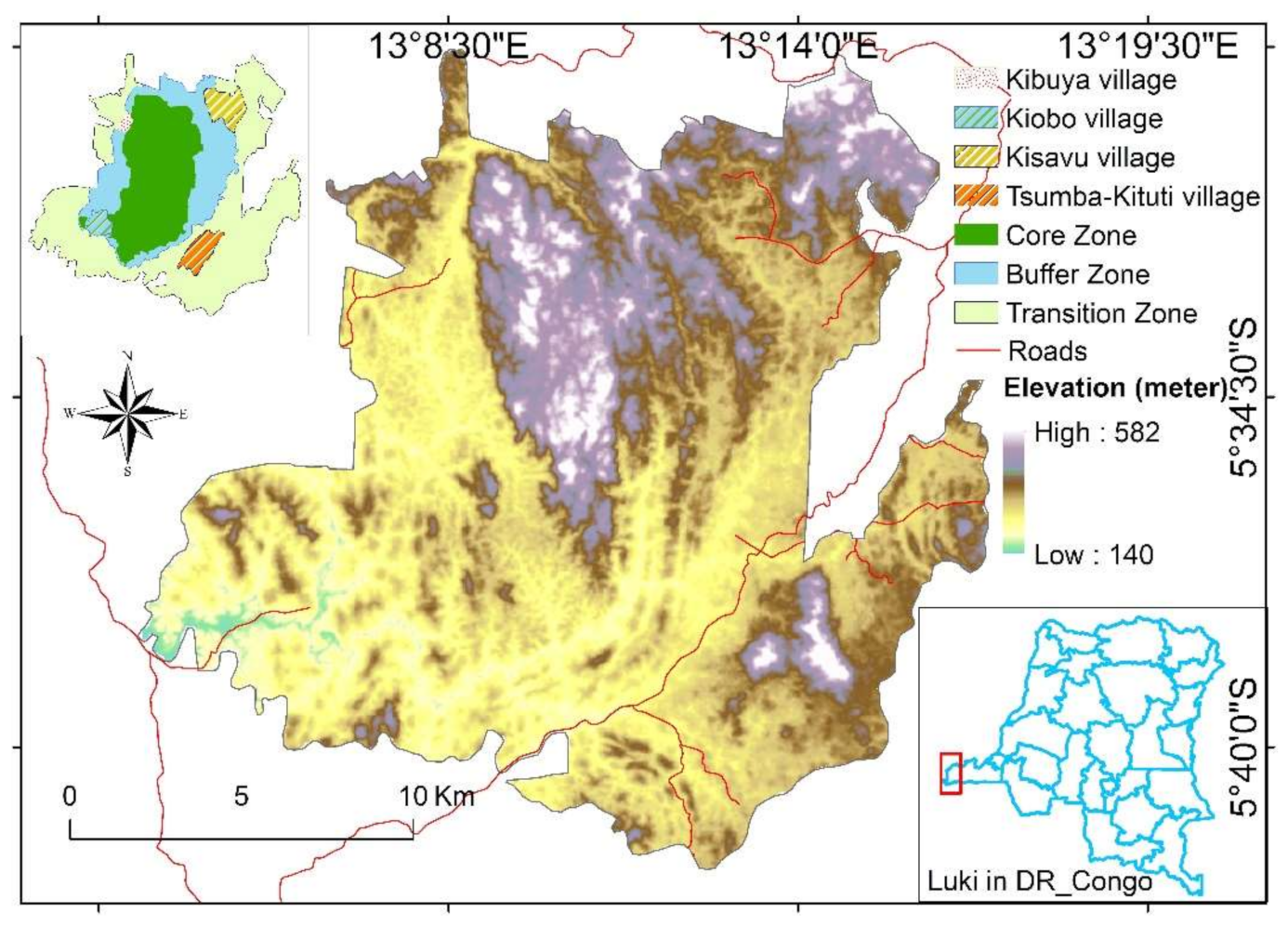
Figure 1. Luki Biosphere Reserve.
Sustainability 13 06898 g001
Figure 2. Annual variation of (a) precipitation and (b) temperature from 1901 to 2019 [41].
Sustainability 13 06898 g002
Figure 3. Multilayer neural network architecture [55].
Sustainability 13 06898 g003
Figure 4. Explanatory variables (a) slope, (b) distance from farmland, (c) distance from villages, (d) distance from roads, (e) elevation.
Sustainability 13 06898 g004
Figure 5. The workflow of the training and simulation processes.
Sustainability 13 06898 g005
Figure 6. Land use/land cover maps for years (a) 1987, (b) 2002, and (c) 2020.
Sustainability 13 06898 g006
Figure 7. Evolution of land use/cover from 1987 to 2020 (a) Core area, (b) Buffer area, (c) Transition area.
Sustainability 13 06898 g007
Figure 8. Landscape metrics (patch cohesion index, aggregation index, and landscape division) in the Luki Biosphere Reserve for the years 1987, 2002 and 2020.
Sustainability 13 06898 g008
Figure 9. Village expansion in the Luki Biosphere Reserve from 1987 to 2020: (a) Tsumba-Kituti, (b) Kisavu, (c) Kiobo, (d) Kibuya.
Sustainability 13 06898 g009
Figure 10. Gradient direction maps of typical villages in the Luki Biosphere Reserve in 1987, 2002, and 2020, respectively (from left to right): (ac) Tsumba-Kituti; (df) Kisavu; (gi) Kiobo; (jl) Kibuya.
Sustainability 13 06898 g010aSustainability 13 06898 g010b
Figure 11. CONTAG index in the Luki Reserve and within different zones.
Sustainability 13 06898 g011
Figure 12. Prediction maps for (a) 2017, (b) 2038.
Sustainability 13 06898 g012
Table 1. Landsat data description.
Data TypeNamePixel SizeWavelengthDescriptionYear
Landsat 4 TMB130 m0.45–0.52 µmBlue1987
B230 m0.52–0.60 µmGreen
B330 m0.63–0.69 µmRed
B430 m0.76–0.90 µmNear infrared
B530 m1.55–1.75 µmShortwave infrared 1
B630 m10.40–12.50 µmThermal Infrared 1.
B730 m2.08–2.35 µmShortwave infrared 2
Landsat 7 ETM+B130 m0.45–0.52 µmBlue2002
B230 m0.52–0.60 µmGreen
B330 m0.63–0.69 µmRed
B430 m0.77–0.90 µmNear infrared
B530 m1.55–1.75 µmShortwave infrared 1
B630 m10.40–12.50 µmLow-gain Thermal Infrared 1
B630 m10.40–12.50 µmHigh-gain Thermal Infrared 1
B730 m2.08–2.35 µmShortwave infrared 2
B815 m0.52–0.90 µmPanchromatic
Landsat 8 OLI/TIRSB130 m0.43–0.45 µmCoastal aerosol2017 and 2020
B230 m0.45–0.51 µmBlue
B330 m0.53–0.59 µmGreen
B430 m0.64–0.67 µmRed
B530 m0.85–0.88 µmNear infrared
B630 m1.57–1.65 µmShortwave infrared 1
B730 m2.11–2.29 µmShortwave infrared 2
B815 m0.52–0.90 µmBand 8 Panchromatic
B915 m1.36–1.38 µmCirrus
B1030 m10.60–11.19 µmThermal infrared 1
B1130 m11.50–12.51 µmThermal infrared 2
Table 2. Cramer’s V test results for the explanatory variables tested in the land use/land cover modeling.
Explanatory VariableCramer’s Vp-Value
Distance from roads0.40970.0000
Distance from villages0.23720.0000
Distance from farmland0.32540.0000
Slope0.16240.0000
Elevation0.32810.0000
Table 3. Landscape metrics used in this study.
DefinitionDescriptionReference
DIVISION = 1 i = 1 n a i j A 2 aij = area (m2) of patch ij.
A = total landscape area (m2).
[74,75,76]
COHESION = 1 j = 1 n p i j j = 1 n p i j a i j x 1 1 Z 100 pij* = perimeter of patch ij in terms of number of cell surfaces.
aij* = area of patch ij in terms of number of cells.
Z = total number of cells in the landscape.
[77]
AI = g i i m a x g i i 100 gii = number of like adjacencies (joins) between pixels of patch type (class) I based on the single-count method.
maxgii = maximum number of like adjacencies (joins) between pixels of patch type (class) i based on the single-count method.
[78]
CONTAG = 1 + i = 1 m k = 1 m P i g i k k = 1 m g i k l n P i g i k k = 1 m g i k 2 l n m Pi = proportion of the landscape occupied by patch type (class) i.
gik = number of adjacencies (joins) between pixels of patch types (classes) i and k based on the double-count method.
m = number of patch types (classes) present in the landscape, including the landscape border if present.
[79]
Table 4. Verification values for classification accuracy.
LULC Categories198720022020
Producer’s Accuracy (%)User’s Accuracy (%)Producer’s Accuracy (%)User’s Accuracy (%)Producer’s Accuracy (%)User’s Accuracy (%)
Primary forest90.791.993.996.399.0598.05
Savannah86.786.793.391.389.2897.16
Secondary forest89.790.291.194.292.394.1
Fallow land and fields92.390.694.792.396.1975.75
Built-up area90.390.391.791.798.4866.41
Overall accuracy (%)89.16 93.6 97.17
Kappa coefficient0.86 0.91 0.92
Table 5. Area statistics for 1987, 2002 and 2020.
LULC Categories198720022020
Area/haArea (%)Area/haArea (%)Area/haArea (%)
Primary forest28842.287.5925781.1978.2924030.2772.02
Secondary forest1959.25.953080.139.33129.179.38
Savannah491.11.49648.751.97577.581.73
Fallow land and fields1584.54.813353.210.185505.0516.5
Built-up area52.80.1666.60.2120.30.36
Table 6. Transition matrix (in %) from 1987 to 2038 in the whole Luki Biosphere Reserve.
Land Use ClassPrimary ForestSecondary ForestSavannahFallow LandBuilt-Up Area
1987 to 2020Primary forest82.124.060.4813.260.08
Secondary forest0.00590.880.7997.8650.45
Savannah0.0007.982483.4491.5567.012
Fallow land0.2677.460.34691.4180.510
Built-up area0.00002.5559.0000.85287.5639
1987 to 2038Primary forest80.39713.15770.278116.06900.0980
Secondary forest0.129073.79751.068923.94031.0643
Savannah0.222010.693848.270129.713211.1008
Fallow land0.871811.67520.541386.37610.5356
Built-up area0.34073.91825.45147.155083.1346
Table 7. Statistics of land use/cover in the Core area from 1987 to 2020.
Land Use CategoryArea in 1987%Area in 2002%Area in 2020%
Fallow land and fields33.90.458.90.7228.42.7
Primary forest8488.698.88383.2397.68201.195.4
Secondary forest69.80.8150.171.7162.81.9
Total8592.31008592.3100.08592.3100.0
Table 8. Statistics of land use/cover in the Buffer area from 1987 to 2020.
Land Use CategoryArea in 1987%Area in 2002%Area in 2020%
Built-up 1.80.033.870.064.590.07
Savannah3.060.053.90.069.980.16
Fallow land and fields176.882.78540.628.5881.6113.88
Primary forest6022.7494.85567.0287.685203.7681.91
Secondary forest148.782.34237.853.7253.323.98
Total6353.26100.06353.26100.06353.26100.0
Table 9. Statistics of land use/cover in the Transition area from 1987 to 2020.
Land Use CategoryArea in 1987%Area in 2002%Area in 2020%
Built-up 50.450.362.50.35115.280.64
Savannah484.242.7643.853.58556.633.1
Fallow land and fields1380.517.72765.7915.364335.1424.1
Primary forest14,344.6679.711,832.8165.7310,304.1157.2
Secondary forest1743.269.72698.1714.992691.9614.96
Total18,003.12100.018,003.12100.018,003.12100.0
Table 10. Components of agreement and disagreement.
Name of ComponentModel
MLP Markov
Persistence simulated correctly95.62%
Change simulated correctly0.79%
Total agreement96.40%
Change simulated as persistence1.91%
Persistence simulated as change1.66%
Change simulated as change to incorrect category0.02%
Total disagreement3.60%
Publisher’s Note: MDPI stays neutral with regard to jurisdictional claims in published maps and institutional affiliations.