Abstract
In this study, discrete choice models that combine different behavioural rules are estimated to study the visitors’ preferences in relation to their travel mode choices to access a national park. Using a revealed preference survey conducted on visitors of Teide National Park (Tenerife, Spain), we present a hybrid model specification—with random parameters—in which we assume that some attributes are evaluated by the individuals under conventional random utility maximization (RUM) rules, whereas others are evaluated under random regret minimization (RRM) rules. We then compare the results obtained using exclusively a conventional RUM approach to those obtained using both RUM and RRM approaches, derive monetary valuations of the different components of travel time and calculate direct elasticity measures. Our results provide useful instruments to evaluate policies that promote the use of more sustainable modes of transport in natural sites. Such policies should be considered as priorities in many national parks, where negative transport externalities such as traffic congestion, pollution, noise and accidents are causing problems that jeopardize not only the sustainability of the sites, but also the quality of the visit.
1. Introduction
The number of nature-based recreational trips has grown significantly in recent years. As a consequence, transport management in natural sites has become crucial in the political agenda, and thus there is a necessity for demand studies that focus on obtaining monetary valuations of travel time and quantify the impact of changes on the choice of different modes of transport (elasticities).
Managers of natural sites around the world are implementing policies to encourage the use of Alternative Transportation Systems (ATS), together with applying dissuasive measures to the use of private cars [1,2]. Yosemite is considered one of the best examples, with the transport system acting as a bridge between the use and the preservation of the park. [3,4,5,6]. Other examples of transport practices in natural sites are Denali (USA) [7,8,9], Rocky Mountains (USA, Canada) [10,11,12,13], Acadia (USA, Canada) [14,15,16] and Zion (USA) [14,17].
Mobility in natural spaces needs a differential analysis because it differs from urban mobility in terms of travel motivations, time valuations and space-time patterns. Particularly, in a recreational demand context, it is imperative to ascertain whether the behavioural rules of the visitors are different to those applied in, for example, an urban mobility context, where the mobility is compulsory for work or study reasons. Despite its relevance, this topic has not been analysed in depth in the literature.
The aim of this paper is to evaluate different behavioural rules to analyse the visitors’ preferences in the choice of access mode to Teide National Park (TNP) (Tenerife Island, Spain) and the extent to which these rules affect the value of travel time savings and elasticities. We start from the hypothesis that examining the visitors’ preferences from different decision rules can be a more suitable approach to deepen our knowledge of the underlying travel mode choice behaviour.
Specifically, we estimate discrete choice models using a hybrid specification that allows us to treat some attributes under conventional linear-additive utility maximization rules (RUM) and others under regret-minimization rules (RRM). In this way, RRM is under the framework of the growing literature on non- and semi-compensatory travel choice models [18]. Although the concept of regret has been extensively used in other disciplines (see for example, [19]), its inclusion in discrete choice models has happened relatively recently in transport literature [20,21,22]. Our analysis is based on a revealed preference (RP) survey conducted on visitors of Teide National Park.
As far as we know, there are no antecedents in the literature of travel mode choice applications that have simultaneously used heterogeneous behavioural rules in the context of mobility in a natural site. Moreover, we contribute to the body of knowledge by comparing monetary valuations of travel time and direct choice elasticities obtained from our best hybrid model with those obtained from a traditional utility maximization framework.
Furthermore, the calculation of the travel time values deserves special mention in this study for two key reasons. First, traditionally, the most used approach in the recreational demand literature to calculate these values has been to approximate them to a fraction of the wage rate (see, e.g., [23,24], approach supported by [25] in the time allocation model proposed by [26]). However, this approach has not been absent of criticism [27] due to the fact that in a recreational trip, the most important measure is not the working time valuation but instead the leisure time valuation. In this study, the value of time is obtained in a rather different way. Specifically, it is derived from the trade-off between money and time that visitors reveal when they choose the mode of transport to access the natural site, an approach consistent with the time allocation theory [28] and the microeconomic model of discrete choices [29]. Second, despite under a random utility maximization framework, the derivation and interpretation of the values of travel time is straightforward, the random regret minimization framework introduces some deviations from this conventional specification that should be considered. Specifically, in our hybrid model, we calculate the values of travel time using the measures proposed by [30,31].
The rest of the work is structured as follows. Section 2 presents the theoretical framework of our choice modelling approach. In Section 2.1, we present the calculation of the values of travel times and elasticities under a RRM framework. In Section 3, we explain the characteristics of TNP along with a descriptive examination of the data collected in the revealed preference survey. Section 4 shows and discusses the main estimation results. Finally, the last section presents the main conclusions.
2. Theoretical Framework
The most widely used theoretical framework for building discrete choice models is the time allocation theory [28] and the microeconomic model of discrete choices [29].
The analysis presented here considers a hybrid model based on both random utility maximization and random regret minimization decision rules. The RRM model proposed by [32] represents an alternative approach to the traditional RUM model [33,34], which has grounded for decades the field of choice modelling in a wide variety of areas, including transportation, health, tourism and environmental economics, among others.
Considering the RUM framework, individuals are utility maximisers, and therefore, given a finite set of options, they choose the one that maximizes their utility. An individual’s utility is considered as a latent construct [35] that the analyst cannot observe and represents the preferences of the individual. Thus, it is separated into two components: (i) a systematic or measurable part that is explained by the attributes of the alternatives and a set of covariates representing the individual’s sociodemographic profile; and (ii) a random term accounting for unobserved effects. Different discrete choice models can be built by considering assumptions about the error structure, among the most popular being the multinomial Logit, the nested Logit and the mixed Logit. The study in [36] presents a comprehensive reference guide for the most widely used RUM models.
The RRM approach considers that individuals are regret minimizers instead of utility maximizers. Thus, it is possible to create a discrete choice modelling framework based on the regret minimization decision rule. The concept of regret is not new in the literature. Originally, it appears in economics and psychology research and nowadays there exist applications to many different fields. The authors of [37] propose the theory of regret regulation by providing a set of ten propositions that capture the current state of art regarding regret. More recently, [30] incorporates the behavioural notion of regret to a discrete choice modelling framework where decision makers evaluate multi-attribute alternatives. In this context, regret appears when non-chosen alternatives have a better performance than the chosen alternatives in some attributes. Thus, when the individuals face the choice among a set of alternatives, they wish to avoid situations causing regret, i.e., when the chosen option is outperformed by other alternatives in some attributes. The authors of [30] provide a set of behavioural intuitions that characterize the anticipated regret of an alternative formalizing the random regret function as:
where is the total regret related with the alternative i, is the observable or systematic regret related with i and is an error term that captures the unobserved heterogeneity in regret of the alternative i.
There are different specifications for in the literature (the interesting website (https://www.advancedrrmmodels.com/, accessed on 21 May 2020) developed by Prof. Sander van Cranenburgh presents an overview of the most advanced RRM models where the reader can consult their specification and main characteristics), but the most extensively used is that proposed in [21], where the observable regret is defined as follows:
where are the unknown parameters related with attribute ; and are the values of attribute for the alternatives j and m, respectively.
The process of choosing the alternative with lowest anticipated regret is much more sophisticated than that of selecting the alternative associated with the maximum utility. In the latter, comparisons are made at the aggregate utility level, whereas in the former, comparisons between alternatives entail comparisons between attributes to determine partial regrets and posterior aggregate regret comparisons.
The choice probabilities in the RRM framework can be derived in a similar way to those obtained from RUM. Thus, assuming that the negative of are iid Extreme Value, and knowing that the minimization of the random regret corresponds to the maximization of its negative, the probability of choosing alternative i is obtained in a similar fashion than that in the RUM multinomial logit model (MNL), and is represented by:
Although there exist many similarities among the RUM and RRM-based MNL model, important differences can be found between them (see [38,39] for further discussion). One of them is that the RRM-based MNL is not grounded on the property of independence from irrelevant alternatives (IIA). This fact makes this model less restrictive, in terms of its application, than the RUM counterpart. Thus, the attractiveness of an alternative depends not only on its own attributes but also on how the attributes of competing alternatives perform when compared with it.
Also, the RRM implies semi compensatory behaviour because a worsening in one attribute is not fully compensated by an improvement in another. The compensation rather depends on how the alternative is positioned in comparison to other alternatives regarding these two attributes. This characteristic has important implications for policy analysis as the same policy could yield forecasts that differ substantially from those obtained within the RUM framework.
Some authors have shown that both RUM and RRM decision rules can be accommodated into the same model [38]. In this context, a hybrid specification can be considered, in which some attributes are assumed to be evaluated by the individuals according to the conventional utility maximization approach whereas others evaluated according to the regret minimization. Thus, a hybrid utility–regret (HUR) function can be built where, without loss of generality, the first Q attributes are specified outside the regret function, and the remaining M-Q inside it. In this case, assuming a linear-additive form for the random utility part, the systematic component of alternative i would be represented by the following expression:
In this case, choice probabilities are computed similarly, yielding the expression:
2.1. Marginal Effects, Willingness to Pay and Elasticities
2.1.1. Marginal Effects
Whereas under the RUM framework obtaining marginal utilities is quite straightforward, RRM marginal effects present a more complex form. Given that the attribute appears in the regret function of all the alternatives, the marginal regrets of alternatives with respect to attribute would take the following form:
which depends not only on the associated coefficient but also on the value of attribute in all the alternatives, in the form of differences and , respectively, differently from the linear-additive RUM where marginal effects are fixed values. It is also interesting to note that represents an upper or lower bound (depending on the sign of the parameter, which is expected to coincide with that obtained from RUM) for each term on the left-hand side expression above; i.e., the absolute value of could be interpreted as an upper bound for the increasing in the regret function associated to alternative j due to a marginal worsening in , or similarly, a lower bound for the regret reduction associated to alternative j due to a marginal improvement in .
In addition, it is also worth pointing out that the magnitude of both the regret and the marginal regret is conditioned by the number of alternatives available to the individual. Therefore, there exists a “choice set (size) dependency” since the larger the choice set, the larger the number of terms included in the regret and marginal regret functions [31]. This is especially relevant for RP data sets, such as the one used in this research, where the set of available alternatives could vary across individuals.
2.1.2. Willingness to Pay
The derivation of the value of time and other willingness to pay (WTP) measures in the context of RUM has a solid microeconomic basis built on the time allocation theories (see [40] for a review of time allocation models) and the microeconomics of discrete choices [29]. Thus, the WTP for improving the attribute in alternative i is obtained as the ratio between the marginal utility of the attribute and the marginal utility of the cost , being the conditional (on the choice of alternative i) indirect utility function [29]. Moreover, this ratio coincides with the negative of the marginal rate of substitution (MRS) between and ; in other words, the negative of the slope of the indifference curve of .
Under the RUM approach, and since the alternatives’ utility is explained only by their own attributes, the willingness to pay also coincides with the quotient between the marginal utilities obtained from the unconditional utility. This function is represented by the expected maximum utility (EMU), which is the utility experienced by an average consumer representative of the population. Under the assumptions of the multinomial Logit model, the expected maximum utility is represented by the well-known LogSum formula, widely used in welfare analysis [41].
The above expression indicates that the marginal rate of substitution between and for the user of alternative i coincides with that of the representative consumer.
When the RRM approach is used, [38] points out that there is not such a “clear conceptual and formal link” between the marginal effect ratios and the willingness to pay. In this case, attributes of competing alternatives enter in the specification of the regret of alternative i, and the regret of the representative consumer for the RRM MNL model is represented by the expected minimum regret (EMR), which equals . Thus, the marginal rate of substitution for the representative consumer no longer coincides with that of users of alternative i, yielding the following two candidate measures for the marginal rate of substitution between and .
An excellent discussion about the pros, cons and properties of these two measures can be found in the study detailed in [31]. The left-hand side term in the above expression was proposed in [30,32] as the regret-based counterpart WTP measure. It is based on the conditional indirect regret function and represents the negative of the marginal rate of substitution between and along the level curve of . As both improvements and deteriorations in an attribute affect the regret of all the alternatives in the choice set, even keeping constant, the individual could change his choice after changing the attribute because of reductions produced in the regret of competing alternatives. Therefore, this measure is valid as long as the marginal changes in the attribute do not provoke changes in the individual’s preferred option. Throughout this paper, we refer to this RRM based measure as the Chorus WTP measure ().
The right-hand term in Equation (8) was proposed by [31] as an alternative to the Chorus measure. It is based on the EMR and, as can be observed in the following expression, the marginal effects of the EMR incorporate the effect of changes in the regret of all the alternatives caused by changes in .
where and are defined as in Equation (3); and and defined as in Equation (6).
It is important to note that the right-hand term in Equation (9) could result in either a positive or negative figure since it is made up of the sum of positive and negative terms. In this regard, positive and negative willingness to pay figures could be obtained when the Dekker measure is used, indicating that some consumers could be benefited after the application of a particular policy, while others could be worse off. Moreover, inordinately high figures could be obtained when the denominator in the WTP expression is close to zero. This has been pointed out by Dekker as one of the main drawbacks of this measure which questions its empirical application.
When the hybrid formulation is considered, the way in which each attribute is processed must be taken into account and the Chorus and Dekker measures can be easily extended by using the appropriate marginal effects. Thus, the marginal effects of the used in the Chorus measure are defined as follows.
The marginal effects of used in the Dekker measure are defined as follows.
2.1.3. Elasticities
Model elasticities can also be derived by computing . They represent the percentage change in due to 1% change in the attribute . Thus, direct and cross elasticities are obtained when and , respectively. The authors of [39] obtained the elasticity formulas for the RRM MNL model. The authors point out that, contrarily to the RUM MNL model, some reversal signs could occur in this case due to the functional form of the regret function.
3. Data and Context
The data used to estimate the models of this paper come from a revealed preference survey conducted on visitors of TNP. The survey was designed to examine the preferences of the visitors in relation to the mode of transport for accessing the park. With an RP survey, we are interested in capturing relevant information about the actual behaviour of the visitors in their trip to the park. TNP is situated in Tenerife, the biggest island of the Canary Islands (Spain). The park is one of the most famous parks in Spain in terms of number of visits and one of the most famous in the world, currently attracting more than five million visitors per year.
According to data from TNP authorities, around 70% of visitors use cars to reach and visit the park whereas the rest of visitors use tourist buses of organized tours. A low percentage of visitors visit the park using public buses or other means of transport such as taxis or bicycles. There are several factors that might explain this behaviour. First is that the park is crossed by a road that concentrates the main landmarks (e.g., the cable car, the visitor centre and the viewpoints) and that, by law, cannot be closed or turned into a toll road. Second is that all the aforementioned landmarks have free parking spaces. Third is that the public bus line reaches the park, but it departs from just two places on the island, has only one departure and return time and can be only used to access the park but not to visit it, because passengers can only get off the bus at one stop. This mobility pattern along with the increasing number of visitors is causing traffic congestion, accidents, noise, pollution and so on, which are negative externalities more related to urban areas than to natural sites. In view of this situation, the implementation of alternative transportation systems to visit the park is mandatory and so is collecting information about visitors’ preferences.
In our RP survey, we collected information about the preferences of 801 visitors. The questionnaires were randomly administered face to face and in different languages to visitors in the most popular landmarks during summer 2016. The survey was composed of three parts. First, socioeconomic questions in relation to their age, gender, nationality, etc. Second, questions regarding their visit to TNP, such as how many times they have visited the park or number of accompanying persons. Third, questions about the trip to the park, that is, the mode of transport they chose, the reason for the choice, the travel times and the travel costs. Although information was collected from about 801 visitors, we restrict the sample in this work to those individuals who correctly answer the question regarding the origin of the trip and those who are not captives of any mode of transport, meaning that they have more than one transport option to reach the park. We also only consider the modes of transport most used by the visitors because including modes that represent a very small fraction of users (e.g., taxi) would lead to misleading estimations. The final sample is composed of 751 visitors and four possible modes of transport: rental/private car and public/tourist bus. Table 1 shows some relevant characteristics of the visitors and of their trip to TNP, as well as the transport mode choices.

Table 1.
Characteristics of the sample and transport mode choices.
Table 1 shows that most of the visitors are from Spain (more than 40%), followed by Germans and British. The most representative age range is situated between 31 and 45 years old, although it is noticeable the high percentage (around 30%) of visitors older than 45 years old. Regarding the questions about the visit to TNP, we can see that for more than 80% of the sample it was their first visit and that 45% of people visit the park accompanied by one person. In relation to the mode of transport, the information collected shows that travel by rental car is the most popular option among visitors (75%), followed by tourist buses in organized excursions (16.5%). Private cars are mainly used by residents of the island, who represent a small fraction of the sample. Above all, it is noticeable the low percentage of use of the public bus (around 2%), due to the reasons mentioned above. In comparing these numbers with official statistics on tourist arrivals to Tenerife as well as with information of TNP authorities, we can assure that our sample represents the population of visitors to TNP.
Lastly, Table 2 shows some descriptive statistics in relation to the level-of-service variables that we use to build the hybrid models of Section 4. We present the average and the standard deviation of the travel cost and the travel time variables (in-vehicle time, access time and waiting time) for the four modes of transport considered.
Table 2.
Descriptive statistics of the variables.
Table 2 shows that, to reach TNP, rental cars and private cars are the fastest modes of transportation, substantially faster than public buses and tourist buses. Regarding the travel costs, the private car is the most competitive mode, followed by the public bus and the rental car. We have to note that the travel cost in tourist bus only refers to the trip to TNP and does not include other services usually included in this kind of excursion. Finally, note that waiting and access time (i.e., walking time from the place of accommodation to the bus stop) are only related to the public bus. They were not considered for tourist buses because usually these buses pick up passengers in the place of accommodation of the visitors.
4. Results
Using the information provided by the revealed preference survey described in the previous sections, we estimated a transport mode choice model to analyse visitors’ preferences in their access to Teide National Park. The data set contains four alternatives: private car (CP), rental car (CR), tourist bus (BT) and public bus (BP). For the first three alternatives, preferences are analysed in terms of in-vehicle travel time (TT) and travel cost (C). The public bus also considers access time (AT) and waiting time (WT).
The analysis is based on the construction of a hybrid model in which the behavioural rule is based on both utility maximization and regret minimization, as described in the previous section. Thus, after considering different specifications, the best results were obtained when access time and waiting time were processed according to RUM, whereas travel time, travel cost and the alternative specific constants were processed according to RRM. In addition, the cost was specified as a random parameter following the normal distribution, allowing for the estimation of individual-specific parameters for this attribute. Estimation results corresponding to the hybrid random parameter random utility-random regret (RP RUM–RRM) model are presented in Table 3, which contains the name of the parameter and the attribute, the estimated coefficient, the t-test and tail probability and the parameter confidence interval. All models were estimated using the software NLOGIT 6 [42].
Table 3.
Estimation results for the hybrid RP RUM–RRM model.
All parameters’ estimates were significant considering the 95% confidence level, except for the case of access time that was significant at the 91.0% confidence level and the public bus constant that which was not significantly different from zero. The standard deviation of the cost coefficient was also very significant, indicating the existence of random heterogeneity in the perception of travel cost. Attribute parameters were also estimated with the correct sign confirming the consistency of the results. Attending the sign of the alternative specific constants, results indicate that the private car (acting as the reference) is preferred when the effect of the rest of the attributes is considered negligible.
With the purpose of comparing our results with alternative and more traditional specifications, the estimation results corresponding to the counterpart RUM model are presented in Table 4. Similarly, parameters were estimated with consistent sign and were significant considering the 95% confidence level, with the exceptions of access time that was significant at the 90.2% confidence level, the car rental constant that was significant at the 93.5% confidence level and the public bus constant that was not significantly different from zero to an acceptable confidence level.
Table 4.
Estimation results for RUM model.
In determining which model is statistically superior, we observe that the RUM is slightly better in terms of the log-likelihood, the adjusted rho-squared (for a more detailed description of the adjusted rho-squared measure, see [43] and [44] (p. 282)) and the Akaike information criteria (AIC). However, for a better comparison between the models, we use the Akaike likelihood ratio test [45] which is specially designed to compare non-nested models. The results of this test suggests that the hybrid RUM–RRM model is superior in terms of fit. (Under the null hypothesis that the hybrid RUM–RRM model is the true specification, the probability that the RUM model outperforms the hybrid RUM–RRM specification is bounded by ϕ (−14.43) ≈ 0, being ϕ the standard normal cumulative distribution function, so we fail to reject the null hypothesis. The test states that , where is the adjusted rho-squared and K is the number of parameters in each model, and Z is a positive number (0.1 was considered in this case) controlling differences in fit measures.) It is also worth pointing out that most attribute parameters in the hybrid model are slightly more significant than in the RUM model, and a figure of 0.684 for the adjusted rho-squared index suggests a fairly good fit of the model to the data set. Summing up, we can conclude that the overall fit between the two models considered is relatively similar.
To further deepen the comparison and interpretation of these two specifications, direct elasticities are estimated and presented in Table 5. Elasticity estimates that did not result significant (note that elasticities are obtained as a function of estimated parameters and, as such, are values that could result not significant estimates) were considered as zero. The elasticities represent the percentage variation in choice probability for the mode of transport in the column in response to a 1% change for the attribute in the row and were computed using individual-specific estimates for the cost and considering probability weights in the sample enumeration method [44].
Table 5.
Direct elasticities.
In general, the choice probability in all the alternatives was more elastic for the RUM–RRM model in all the attributes, except for the public bus where the elasticity estimates with respect to time attributes did not result significant. The choice probabilities in the RUM–RRM were more elastic to travel cost than travel time in the bus alternatives, being this figure rather high for the tourist bus. In contrast, probabilities in the RUM model are more sensitive to travel time for the car alternatives and the public bus, whereas for the tourist bus, the time elasticity is lower. This result could be explained by the fact that in tourist buses there could exist some type of entertainment such as a tour guide giving explanations about the route, thus increasing the chances of having a more productive use of time. In addition, the public bus resulted more elastic to access and waiting time than to in-vehicle time.
Value of Time
In this section, the willingness to pay measures for saving travel time in the context of recreational trips are obtained. Figures are computed considering the individual specific estimates for the cost and using probability weights. Aggregate WTP figures are obtained considering the weighted average over the set of individuals who have the alternative available. For this reason, alternative specific figures are obtained also for the RUM model. For the hybrid RUM–RRM model, both Chorus and Dekker WTP measures (see Section 2.1) are obtained considering marginal effects defined as in Equations (10) and (11). Since travel time is measured in minutes and travel cost in euro cents, figures obtained are multiplied by 0.6 in order to transform the value of time units into euros/hour. In addition, for the Dekker measure, separate aggregates are made for individuals with positive and negative WTP, recognizing the fact that the application of this measure could lead to the existence of winners and losers among users of the same mode of transport after the application of a particular policy.
The values obtained for the components of total travel time are presented in Table 6. Regarding the value of travel time (in-vehicle) for car alternatives, similar figures are obtained for the RUM model, the Chorus measure and winners in the Dekker measure, ranging from 5.28 to 6.44 EUR/h. In contrast, for bus alternatives, winners in the Dekker measure exhibit the highest willingness to pay (13.49 EUR/h). It is also worth noting the low value of time (2.67 EUR/h) obtained for tourist bus users when the Chorus measure is used. These results suggest a heterogeneous perception of travel time among our sample of respondents. In addition, since the hybrid RUM–RRM model yields individual specific marginal effects, this formulation provides richer information as it enables researchers to identify differences in visitors’ behaviour even when preference parameters are fixed.
Table 6.
Value of time components.
In the case of access and waiting time, the RUM model and the winners in the Dekker measure present WTP figures that are rather high (23.49 and 49.39 EUR/h for access time and 46.99 and 91.35 EUR/h for waiting time, respectively). These figures made the Chorus measure more attractive as its results are more consistent with that obtained in other studies conducted in the TNP. In this respect, [46] obtained, in the analysis of mode choice for visits inside the park, a willingness to pay of 9.22 EUR/h for saving waiting time for bus users and 10.27 EUR/h for saving time finding parking space for car drivers.
To better understand the meaning of the willingness to pay figures obtained using these three approaches, the distribution of the WTP is analysed through the kernel density estimates shown in Figure 1 and Figure 2. In the case of in-vehicle travel time (Figure 1) for the first three alternatives, the distribution of the Dekker measure (labelled as TTi_RRD) presents a significant proportion of individuals with negative WTP, this being higher for tourist bus users. The distribution of the value of time obtained for the RUM model (labelled as TTi_RU) has less dispersion than that obtained from the Chorus measure (labelled as TTi_RRC). In contrast, for private car users, the value of time distribution does not present negative values and the two approaches used for the hybrid model show similar results. As for the case of access and waiting time (Figure 2), the values of time distributions are substantially different, explaining differences obtained in aggregate measures presented in Table 6. In addition, individuals obtaining negative value of time (in the Dekker measure) suggest that even in the case of marginal reductions in travel time they could claim a monetary compensation to keep the expected maximum hybrid utility–regret function constant.
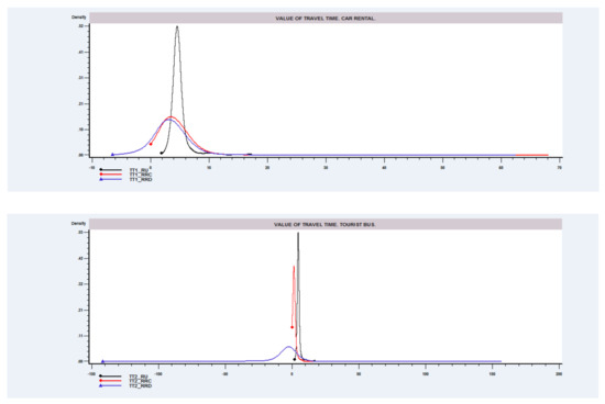
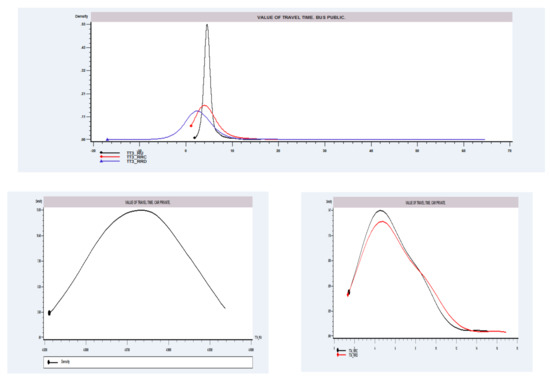
Figure 1.
Value of in-vehicle travel time. Kernel density estimates.
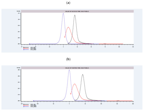
Figure 2.
Value of access and waiting time. Kernel density estimates.
5. Conclusions
A hybrid random-utility-maximization (RUM) and random-regret-minimization (RRM) model could offer a behavioural alternative to a fully compensatory RUM model for studying travel mode choice preferences. This possibility is especially valuable in the context of recreational trips in natural environments, which clearly differ from commuting trips in urban environments. One of the core concepts in transport economics is that transport demand is a derived demand; that is, people in commuting trips do not demand transport “per se”, but rather they demand transport to carry out a particular activity located in time and space such as working or studying. In the case of recreational trips, this concept is partially true because the trip itself can be part of the recreational activity. In this situation, the assumption that the travel mode choice is based on a fully compensatory behaviour in terms of the attributes of the modes of transport can be too restrictive.
In this paper, we estimated a RUM–RRM discrete choice model than combines different behavioural rules to study visitors’ preferences for accessing a national park. Specifically, we present a hybrid model specification that includes random parameters, where some attributes are assumed to be evaluated by the individuals according to the conventional utility maximization approach whereas others were evaluated according to regret minimization. Our application is based on a data set collected from a RP survey of visitors to Teide National Park. We presented the estimation of the hybrid model and, for comparative purposes, the estimation of its RUM model counterpart. For both models, we estimated direct choice elasticities and travel time values using the measures of Chorus and Dekker in the case of the RUM–RRM model. This approach constitutes the first comparison of RUM–RRM and RUM models in a recreational trip context.
Our findings suggest that the overall model fit between RUM–RRM and RUM models is relatively similar. Despite that, the willingness to pay figures and elasticities obtained from both models are different. With respect to the values of travel time, we found first significant differences between the different measures used, and second, more reasonable willingness to pay figures, according to those obtained in previous studies conducted in the same context, when we use the Chorus approximation to obtain the value of time. It is also worth highlighting that in the RUM–RRM model, the marginal effects are no longer fixed values, enabling us to estimate different values of time according to different modes of transport despite specifying generic coefficients for some travel components. Regarding the direct elasticities, and focusing on the modes of transport with the highest market shares in our application (rental car and tourist bus), we found two main results. The first is that the choice probabilities in the RUM–RRM model change more than those in the RUM model when travel cost and travel time are modified. The second is that in both models, rental car users are more sensitive to travel time whereas tourist bus users are more sensitive to travel cost. The first result could be explained as follows: the RRM approach accounts for the chance that the wrong choice might have been made (regret), thus amplifying the behavioural responses in relation to a RUM approach [39]. The second result may be due to the fact that the travel time in a tourist bus might be less relevant than the travel cost because part of it can be considered as pleasant and part of the excursion.
Results obtained in this work provide very useful instruments to evaluate policies aiming to promote the use of more sustainable and efficient modes of transport to access natural sites. These policies should be considered as priorities in areas such as the one studied here (Teide National Park), where negative transport externalities are causing problems that jeopardize not only the sustainability of the area, but also the quality of the visit. For example, different initiatives associated with the implementation of incentives for the use of Alternative Transportation Systems—such as buses, trains, bicycles and cableways—together with applying dissuasive measures to the use of private vehicles, such as tolls and restrictions on car access [1,2]. More specifically, one of these initiatives is the use of e-public transport such as electric buses and electric bikes (see the studies of [46] for an internal electric bus and [47] for e-bike sharing, both studies in Teide National Park), which apart from representing a more sustainable mobility system, it may also become a tourist attraction itself, allowing a more direct contact with the natural heritage.
Our findings reinforce the importance of examining different behavioural rules when analysing visitors’ preferences in a recreational demand context. Travel time values and elasticities obtained with conventional models based only on utility maximization rules could differ from those obtained with potentially more complete hybrid models combining different decision rules. Travel time values and elasticities are essential measures to assess the effects of a transport intervention strategy; thus, an incorrect estimation of these values could lead to wrong valuations of the benefits associated with the implementation of alternative transportation systems in natural parks.
Author Contributions
Conceptualization, R.M.G. and C.R.; methodology, C.R.; formal analysis, R.M.G. and C.R.; investigation, R.M.G., C.R. and Á.S.M.; resources, R.M.G.; data curation, R.M.G. and Á.S.M.; writing—original draft preparation, R.M.G. and C.R.; writing—review and editing, R.M.G., C.R. and Á.S.M.; supervision, R.M.G. and C.R.; project administration, R.M.G.; funding acquisition, R.M.G. All authors have read and agreed to the published version of the manuscript.
Funding
This research was funded by CajaCanarias Foundation for funding the project entitled “Design of a Sustainable Mobility Plan for visitors to the Teide National Park and Evaluation of the Implementation of ‘Cycle’ Lanes in Tenerife”.
Data Availability Statement
The data that support the findings of this study are available on request from the corresponding author.
Acknowledgments
The authors wish to thank the CajaCanarias Foundation for funding the project entitled “Design of a Sustainable Mobility Plan for visitors to the Teide National Park and Evaluation of the Implementation of ‘Cycle’ Lanes in Tenerife”, from which data were extracted for this study. Thanks are also due to the director and technicians of Teide National Park for the documentation and information provided.
Conflicts of Interest
The authors declare no conflict of interest.
References
- Holding, D.M.; Kreutner, M. Achieving a balance between “carrots” and “sticks” for traffic in National Parks: The Bayerischer Wald project. Transp. Policy 1998, 5, 175–183. [Google Scholar] [CrossRef]
- Orsi, F.; Geneletti, D. Assessing the effects of access policies on travel mode choices in an Alpine tourist destination. J. Transp. Geogr. 2014, 39, 21–35. [Google Scholar] [CrossRef]
- Youngs, Y.L.; White, D.D.; Wodrich, J.A. Transportation systems as cultural landscapes in national parks: The case of Yosemite. Soc. Nat. Resour. 2008, 21, 797–811. [Google Scholar] [CrossRef]
- Meldrum, B.; DeGroot, H. Integrating transportation and recreation in Yosemite National Park. In The George Wright Forum; George Wright Society: Hancock, MI, USA, 2012; Volume 29, pp. 302–307. [Google Scholar]
- White, D.D.; Tschuor, S.; Byrne, B. Assessing and modeling visitors’ evaluations of park road conditions in Yosemite National Park. In The George Wright Forum; George Wright Society: Hancock, MI, USA, 2012; Volume 29, pp. 308–321. [Google Scholar]
- Reigner, N.; Lawson, S.; Meldrum, B.; Pettebone, D.; Newman, P.; Gibson, A.; Kiser, B. Adaptive management of visitor use on Half Dome, an example of effectiveness. J. Park Recreat. Adm. 2012, 30, 64–78. [Google Scholar]
- Phillips, L.; Mace, R.; Meier, T. Assessing impacts of traffic on large mammals in Denali National Park and Preserve. Park Sci. 2010, 27, 42–47. [Google Scholar]
- Manning, R.E.; Hallo, J.C. The Denali park road experience: Indicators and standards of quality. Park Sci. 2010, 27, 33–41. [Google Scholar]
- Morris, T.; Hourdos, J.; Donath, M.; Phillips, L. Modeling traffic patterns in Denali National Park and Preserve to evaluate effects on visitor experience and wildlife. Park Sci. 2010, 27, 48–57. [Google Scholar]
- D’Antonio, A.; Monz, C.; Newman, P.; Lawson, S.; Taff, D. Enhancing the utility of visitor impact assessment in parks and protected areas: A combined social–ecological approach. J. Environ. Manag. 2013, 124, 72–81. [Google Scholar] [CrossRef]
- Lawson, S.; Chamberlin, R.; Choi, J.; Swanson, B.; Kiser, B.; Newman, P.; Monz, C.; Pettebone, D.; Gamble, L. Modeling the effects of shuttle service on transportation system performance and quality of visitor experience in Rocky Mountain National Park. Transp. Res. Rec. 2011, 2244, 97–106. [Google Scholar] [CrossRef]
- Park, L.; Lawson, S.; Kaliski, K.; Newman, P.; Gibson, A. Modeling and mapping hikers’ exposure to transportation noise in Rocky Mountain National Park. Park Sci. 2010, 26, 59–64. [Google Scholar]
- Pettebone, D.; Newman, P.; Lawson, S.R.; Hunt, L.; Monz, C.; Zwiefka, J. Estimating visitors’ travel mode choices along the bear lake road in Rocky Mountain National Park. J. Transp. Geogr. 2011, 19, 1210–1221. [Google Scholar] [CrossRef]
- Roof, C.J.; Kim, B.; Fleming, G.G.; Burstein, J.; Lee, C.S. Noise and Air Quality Implications of Alternative Transportation Systems: Zion and Acadia National Park Case Studies; US Department of Transportation: Cambridge, MA, USA, 2002.
- Pettengill, P.R.; Manning, R.E.; Anderson, L.E.; Valliere, W.; Reigner, N. Measuring and managing the quality of transportation at Acadia National Park. J. Park Recreat. Adm. 2012, 30, 68–84. [Google Scholar]
- Hallo, J.C.; Manning, R.E. Analysis of the social carrying capacity of a national park scenic road. Int. J. Sustain. Transp. 2010, 4, 75–94. [Google Scholar] [CrossRef]
- Mace, B.L.; Marquit, J.D.; Bates, S.C. Visitor assessment of the mandatory alternative transportation system at Zion National Park. Environ. Manag. 2013, 52, 1271–1285. [Google Scholar] [CrossRef] [PubMed]
- Cantillo, V.; Ortúzar, J. A semi-compensatory discrete choice model with explicit attribute thresholds of perception. Transp. Res. Part B Methodol. 2005, 39, 641–657. [Google Scholar] [CrossRef]
- Wang, S.; Chorus, C.; Shaheen, S.A.; Walker, J.L. A Revealed Preference Methodology to Evaluate Regret Minimization with Challenging Choice Sets: A Wildfire Evacuation Case Study. Travel Behav. Soc. 2020, 20, 331–347. [Google Scholar] [CrossRef]
- Chorus, C.G.; Arentze, T.A.; Timmermans, H.J.P. A random regret-minimization model of travel choice. Transp. Res. Part B 2008, 42, 1–18. [Google Scholar] [CrossRef]
- Chorus, C. A new model of random regret minimization. Eur. J. Transp. Infrastruct. Res. 2010, 10, 181–196. [Google Scholar]
- An, S.; Wang, Z.; Cui, J. Integrating Regret Psychology to Travel Mode Choice for a Transit-Oriented Evacuation Strategy. Sustainability 2015, 7, 8116–8131. [Google Scholar] [CrossRef]
- Hagerty, D.; Moeltner, K. Specification of driving costs in models of recreation demand. Land Econ. 2005, 81, 127–143. [Google Scholar] [CrossRef]
- Gürlük, S.; Rehber, E. A travel cost study to estimate recreational value for a bird refuge at Lake Manyas, Turkey. J. Environ. Manag. 2008, 88, 1350–1360. [Google Scholar] [CrossRef]
- Cesario, F.J. Value of time in recreation benefit studies. Land Econ. 1976, 52, 32–41. [Google Scholar] [CrossRef]
- Becker, G.S. A Theory of the Allocation of Time. Econ. J. 1965, 75, 493–517. [Google Scholar] [CrossRef]
- Palmquist, R.B.; Phaneuf, D.J.; Smith, V.K. Short run constraints and the increasing marginal value of time in recreation. Environ. Resour. Econ. 2010, 46, 19–41. [Google Scholar] [CrossRef]
- DeSerpa, A.C. A theory of the economics of time. Econ. J. 1971, 81, 828–846. [Google Scholar] [CrossRef]
- McFadden, D. Econometric models of probabilistic choice. In Structural Analysis of Discrete Data: With Econometric Applications; Manski, C., McFadden, D., Eds.; MIT Press: Cambridge, MA, USA, 1981. [Google Scholar]
- Chorus, C. Random regret minimization: An overview of model properties and empirical evidence. Transp. Rev. 2012, 32, 75–92. [Google Scholar] [CrossRef]
- Dekker, T. Indifference based value of time measures for Random Regret Minimisation models. J. Choice Model. 2014, 12, 10–20. [Google Scholar] [CrossRef]
- Chorus, C.G. Random Regret-Based Discrete Choice Modelling: A Tutorial; Briefs in Business Book Series; Springer: Berling, Germany, 2012. [Google Scholar]
- Thurstone, L.L. A law of comparative judgment. Psychol. Rev. 1927, 34, 273–286. [Google Scholar] [CrossRef]
- McFadden, D. Conditional logit analysis of qualitative choice behavior. In Frontiers in Econometrics; Zarembka, P., Ed.; Academic Press: New York, NY, USA, 1974; pp. 105–142. [Google Scholar]
- Louviere, J.J.; Flynn, T.N.; Carson, R.T. Discrete choice experiments are not conjoint analysis. J. Choice Model. 2010, 3, 57–72. [Google Scholar] [CrossRef]
- Train, K. Discrete Choice Methods with Simulation, 2nd ed.; Cambridge University Press: New York, NY, USA, 2009. [Google Scholar]
- Zeelenberg, M.; Pieters, R. A theory of regret regulation 1.0. J. Consum. Psychol. 2007, 17, 3–18. [Google Scholar] [CrossRef]
- Chorus, C.G.; Rose, J.M.; Hensher, D.A. Regret minimization or utility maximization: It depends on the attribute. Environ. Plan. B Plan. Des. 2013, 40, 154–169. [Google Scholar] [CrossRef]
- Hensher, D.A.; Greene, W.H.; Chorus, C.G. Random regret minimization or random utility maximization: An exploratory analysis in the context of automobile fuel choice. J. Adv. Transp. 2013, 47, 667–678. [Google Scholar] [CrossRef]
- Gonzalez, R.M. The value of time: A theoretical review. Transp. Rev. 1997, 17, 245–266. [Google Scholar] [CrossRef]
- Small, K.A.; Rosen, H.S. Applied welfare economics with discrete choice models. Econom. J. Econo-Metr. Soc. 1981, 49, 105–130. [Google Scholar] [CrossRef]
- Greene, W.H. Nlogit Version 6.0 Reference Guide; Econometric Software, Inc.: Plainview, NY, USA, 2016. [Google Scholar]
- Ben-Akiva, M.; Lerman, S. Discrete Choice Analysis: Theory and Application to Travel Demand; MIT Press: Cambridge, MA, USA, 1985. [Google Scholar]
- Ortúzar, J.d.D.; Willumsen, L.G. Modelling Transport, 4th ed.; John Wiley & Sons: Hoboken, NJ, USA, 2011. [Google Scholar]
- Ben-Akiva, M.; Swait, J. The Akaike likelihood ratio index. Transp. Sci. 1986, 20, 133–136. [Google Scholar] [CrossRef]
- González, R.M.; Román, C.; de Ortúzar, J.D. Preferences for sustainable mobility in natural areas: The case of Teide National Park. J. Transp. Geogr. 2019, 76, 42–51. [Google Scholar] [CrossRef]
- González, R.M.; Román, C.; Marrero, A.S. Visitors’ Attitudes towards Bicycle Use in the Teide National Park. Sustainability 2018, 10, 3283. [Google Scholar] [CrossRef]
Publisher’s Note: MDPI stays neutral with regard to jurisdictional claims in published maps and institutional affiliations. |
© 2021 by the authors. Licensee MDPI, Basel, Switzerland. This article is an open access article distributed under the terms and conditions of the Creative Commons Attribution (CC BY) license (https://creativecommons.org/licenses/by/4.0/).