Nonintrusive Residential Electricity Load Decomposition Based on Transfer Learning

Abstract

Monitoring electricity consumption in residential buildings is an important way to help reduce energy usage. Nonintrusive load monitoring is a technique to separate the total electrical load of a single household into specific appliance loads. This problem is difficult because we aim to extract the energy consumption of each appliance by only using the total electrical load. Deep transfer learning is expected to solve this problem. This paper proposes a deep neural network model based on an attention mechanism. This model improves the traditional sequence-to-sequence model with a time-embedding layer and an attention layer so that it can be better applied in nonintrusive load monitoring. In particular, the improved model abandons the recurrent neural network structure and shortens the training time, which means it is more appropriate for use in model pretraining with large datasets. To verify the validity of the model, we selected three open datasets and compared them with the current leading model. The results show that transfer learning can effectively improve the prediction ability of the model, and the model proposed in this study has a better performance than the most advanced available model.

1. Introduction

Nonintrusive load monitoring (NILM) decomposes the power of each electric appliance according to the total load power in a household. This research was first proposed by Professor Hart in the 1980s [1]. NILM is significant for power plants, retailers, and end users. With the rapid development of smart grid and home-energy-management systems, massive residential electricity consumption data and controllable electric appliances provide new opportunities to realize high levels of energy efficiency, energy conservation, and emission reductions. Traditional load decomposition methods identify equipment by seeking changes in signals, such as the voltage, current, and power, and use specific recognition algorithms for load decomposition [2,3,4]. Based on the working conditions of the equipment, signal features can be classified into three types: steady state, transient state, and running mode. These features will reappear over time. This periodic trend constitutes the fundamental principle of load identification [5]. Traditional NILM methods build equipment feature databases by manually extracting features, while deep neural networks can realize automatic learning from data, thereby avoiding the step of manually extracting features [6,7]. As deep learning has been effectively applied in image and voice identification, some people have started to explore its application in NILM. However, deep learning requires a large amount of training data to understand the potential data patterns. Acquiring high-quality NILM training samples in the field is very costly. Usually, a separate metering device is needed to obtain sub-equipment label data. Depending on the acquisition cycle, data can include high-frequency data and low-frequency data. According to ref. [8], the sampling period is macro or micro whenever it is more than or less than 1 s, respectively. High-frequency data can accurately record the micro changes when the equipment state is transitioning, but the need for an additional acquisition device leads to a high transmission and storage cost. Therefore, popularizing the application of high-frequency data is difficult. Depending on the mission target, NILM can be divided into two types: event-detection (ED) and energy-estimation (EE) [9]. The former aims to predict the state of the appliance switch, while the latter aims to predict electricity consumption. Traditional NILM methods decompose energy based on ED, so they are called event-based approaches. In contrast, deep learning achieves decomposition through end-to-end learning, so it is called an event-free approach. The event-based approach, which requires accurate equipment-state identification, is applicable to high-frequency data. Because the event-free approach represented by deep learning can be directly used for load prediction, it is appropriate for low-frequency data. Smart electric meters can collect low-frequency data, which makes the results of NILM research on low-frequency data more applicable in practical applications.

Because deep learning is a representation learning algorithm based on large-scale data, its reliance on scale hinders its application. Transfer learning is an important tool that can be used to solve the problem of insufficient deep learning training data. This approach attempts to transfer knowledge from the source domain to the target domain by assuming that the training data and the test data must be independent and identically distributed. In ref. [10], this knowledge transfer is defined as follows: for a learning task ${\mathrm{T}}_{\mathrm{t}}$ based on data ${\mathrm{D}}_{\mathrm{t}}$, we can obtain useful knowledge for task ${\mathrm{T}}_{\mathrm{s}}$ from ${\mathrm{D}}_{\mathrm{s}}$. Transfer learning aims to improve the performance of prediction function ${\mathrm{f}}_{\mathrm{T}}$ of task ${\mathrm{T}}_{\mathrm{t}}$ by identifying and converting the tacit knowledge in ${\mathrm{D}}_{\mathrm{s}}$ and ${\mathrm{T}}_{\mathrm{s}}$. In particular, ${\mathrm{D}}_{\mathrm{s}}\ne {\mathrm{D}}_{\mathrm{t}}$ and/or ${\mathrm{T}}_{\mathrm{s}}\ne {\mathrm{T}}_{\mathrm{t}}$, and the scale of ${\mathrm{D}}_{\mathrm{s}}$ is usually much larger than that of ${\mathrm{D}}_{\mathrm{t}}$. Deep transfer learning based on neural networks refers to the process of reusing some networks that have been pretrained in the source domain, including network structures and connection parameters, and transferring them to the target domain as a part of the target deep neural network. In fact, this kind of transfer learning imitates the processing mechanism of the human brain. The network closest to the input end can extract the general features at the bottom layer, while that near the output end uses features of the bottom layer to predict specific tasks [11]. Refs. [12,13] pointed out the relationship between the network structure and transferability, specified which features can be transferred in the deep network and demonstrated that network structures such as LeNet, AlexNet, VGG, Inception and ResNet are applicable to deep transfer learning through an experiment. At present, most research on transfer learning has been conducted for supervised learning. Determining how to use deep neural networks for unsupervised or semi-supervised transfer learning is still very difficult.

2. Deep Transfer Learning and NILM

For the application of deep-learning technology in NILM, ref. [14] was the first to propose three deep neural-network architectures that can be used to solve the NILM problem, i.e., long short-term memory (LSTM), denoising autoencoders (DA), and Rectangles, and to verify them in the public dataset UK-DALE [15]. Recent studies have proven that the deep neural-network model is better than the traditional combinatorial optimization (CO) model and the factorial hidden Markov model (FHMM), especially in terms of the generalizability, which is the weakness of traditional models [16,17]. However, simple recurrent neural networks (RNNs), such as the LSTM, cannot learn from equipment with multiple states and long power-changing intervals, as this will lead to a vanishing gradient [18,19]. The sequence-to-sequence (seq2seq) model is a general end-to-end training approach that maps the input sequence into the output sequence through the encoder-decoder structure. This model solves the problem in which traditional neural networks cannot map a sequence into a sequence. In the literature, ref. [20] was the first to propose the seq2seq model and use it for text translation, and the effects were remarkable. Similarly, ref. [14] was the first to use the seq2seq model to solve the NILM problem and demonstrate that this model can identify a target appliance from total power signals. This result is significant because it illustrates that complex electrical features can be automatically extracted through deep neural networks, which settles the problems related to the difficult manual extraction of features and the low efficiency. However, the seq2seq model has its limitations. When there is a long input sequence, it cannot memorize the state information in the distance, which lowers the prediction accuracy. For example, there are several seconds or minutes between the start-up periods of the different working stages of a washing machine, including washing, dewatering, and drying, which can cause the model to lose information. Generally, a sliding window may be used to solve this problem. A window of a certain length can be selected, and then by using this window, the input signals can be divided into sequences and mapped into the output window. However, when the sliding window is used for prediction, each final output point is the mean of multiple predictions, which can make the prediction value at the edge of a window smooth and thereby lower the prediction accuracy. Through research, ref. [21] improved the seq2seq model and proposed the seq2point model. This model changes the output from predicting one sequence to predicting a single point and uses a one-dimensional convolutional neural network (CNN) as the encoder for training. The results showed that the CNN is capable of learning the features of target signals, which significantly increases the ability of this model. If Y(t:t + w − 1) represents the window sequence input into the model at moment t, then the seq2point model only predicts the output at moment t + (w/2). As a result, the model concentrates its expressing ability on the middle points of the window, thereby fully utilizing the information of adjacent front and back areas to improve the prediction accuracy.

Deep neural networks are able to effectively extract general features from the bottom layer that can also be used to predict other problems of the same kind. This transfer learning approach has been widely applied in image identification, natural language processing, and other areas [11,13]. Currently, the research on the application of transfer learning in NILM is limited. Ref. [22] classified NILM transfer learning into two types—appliance transfer learning (ATL) and cross-domain transfer learning (CTL)—and used the seq2point model for training and transfer learning in several public datasets. The results showed that for ATL, the pattern learned by a complex appliance (e.g., washing machine) can be transferred to a simple appliance (e.g., kettle). For CTL, the seq2point model is also capable of transfer learning. When the training and test data are located in similar domains, it can be applied to test data without fine-tuning. However, if the training and test data are located in different domains, fine-tuning is necessary. The experimental results also showed that fine-tuning the fully connected layer alone achieves a good effect. The major structure of the seq2point model is a one-dimensional convolutional layer, which indicates that a convolutional network is appropriate for transfer learning. This conclusion is consistent with the research on transfer learning in image identification. However, power load data are typical time sequences. The numerical value at a certain moment has a close relationship with the values at adjacent moments. Therefore, we present in this paper a new model that increases the prediction ability of the seq2seq model by introducing an attention mechanism.

3. Transfer Learning Based on an Attention Model

3.1. Attention Model

Attention, also called an attention mechanism, is similar to the manner in which the human brain ignores unimportant information and focuses on important information when processing information. The key is to compute and allocate attention scores to concentrate attention on relevant content and thereby increase its contributions. Ref. [23] proposed the initial attention mechanism, which enables the machine translation model to automatically search and predict target term-related source statements for translation. This approach uses variable context vectors to solve the problem in which the seq2seq model loses information and leads to inaccurate predictions when there is a long sequence. Ref. [24] proposed two types of attention mechanisms: a global attention mechanism, which focuses on all source words, and a local attention mechanism, which focuses on a portion of source words. The attention score, which is an important concept in attention models, can measure the significance of each character in the input sentence to each character in the target sentence. This score can be obtained through a substantial amount of sample training. With the attention mechanism, the seq2seq model shows a large improvement in translating long sentences [24]. In essence, the models proposed in ref. [14,21] are also seq2seq models. The decoder only utilizes the final state information of input sequences without considering the influence of their different locations on the output. The model mentioned herein is actually the seq2seq model that contains an attention mechanism. It has been changed to an attention model. Figure 1 explains how the attention mechanism works.

Depending on the length of the input and output sequences, the seq2seq model has three forms: many-to-many, many-to-one, and one-to-many [20]. The attention mechanism was first implemented in the many-to-many model [25]. The attention score of this model can be calculated as $h_{t}W\overline{h_i}$ where $h_t$ is the current decoding state of the decoder, and $\overline{h_i}$ is the hidden state of the encoder. However, there is no $h_t$ in the many-to-one model. If we deem the many-to-one problem as a special form of the many-to-many problem, then $h_t$ can be replaced with the last hidden state $h_{last}$ of the encoder. As shown in Formula (1), tensor W is a square matrix with a hidden size of the encoder. The parameters in this matrix are obtained through model training. The final output ${\mathrm{y}}_{\mathrm{i}}$ of the model uses the context vector and the final hidden state of encoder as the inputs for decoding. The context vector (Formula (2)), which is the core of the model, is the weighted sum of the attention weight $w_{ti}$ and the hidden state $\overline{h_i}$ of the encoder. In particular, the attention weight (Formula (3)) refers to the contribution made by the values of input sequence at different locations to the prediction of the current output ${\mathrm{y}}_{\mathrm{i}}$, which indicates that the different input locations may be referenced to varying degrees. Generally, both the encoder and the decoder use an RNN, which relies on the output of the last moment for computation. Thus, parallel computing cannot be realized, thereby leading to a very long period of model training. The model mentioned herein replaces the RNN with the embedding layer Time2Vector and the attention layer. Time2Vector is a method for processing time sequences proposed by ref. [26]. It can learn time features and conduct parallel computing, thereby accelerating model training. Because ref. [21] demonstrated that predicting the points in the middle of the output window alone is more accurate than predicting the entire output sequence, the model herein uses the many-to-one form.

$$\begin{array}{c}\begin{array}{c}score\left(h_{last},{\overline{h}}_i\right)={h_{last}}^{\top }W{\overline{h}}_i\end{array}\end{array}$$

(1)

$$\begin{array}{l}{c}_t={\displaystyle \sum _i}{w}_{ti}{\overline{h}}_i\hfill \end{array}$$

(2)

$$w_{ti}=\frac{\exp \left(score\left(h_{last},{\overline{h}}_i\right)\right)}{{{\displaystyle \sum }}_{i^{\prime }=1}^I\exp \left(score\left(h_{last},{\overline{h}}_{i^{\prime }}\right)\right)}$$

(3)

The seq2point model is composed of five one-dimensional convolutional layers and two fully connected layers [21]. Its specific structure is shown Figure 2. Because it uses a CNN, which can conduct parallel computing, this model has a high training speed. The attention model mentioned herein replaces the RNN with the time embedding layer as the encoder. The concatenate layer connects the embedding layer with the input layer and then sends them to the attention layer, and the two fully connected layers function as a decoder, as shown in Figure 3. Because the model finally predicts a point rather than a sequence, the activation function of the last layer FC-1 is linear, and the other layers use the rectified linear unit (ReLU). This approach has been demonstrated to provide the optimal solution in previous research [21,27,28].

3.2. Approaches to Transfer Learning

In the literature, ref. [12] was the first to study the transferability of deep neural networks. They divided the ImageNet dataset containing 1000 categories into two parts: A and B. Then, they trained an eight-layer neural network for A and B and conducted a fine-tuning experiment from layers 1–7 to explore the transferability of the network. This paper uses two approaches to transfer learning. The first approach, AnB, fixes the first n layers of network A, randomly initializes the remaining layers, and then classifies B; the other approach, BnB, fixes the first n layers of network B, randomly initializes the remaining layers, and then classifies B. The experimental results of this paper show that (1) the first three layers of the neural network all have general features, which are good for transfer; (2) fine-tuning the deep transfer network can greatly improve the effect, even better than the original network (based on B’s own training); and (3) fine-tuning can resolve the difference between data. Fine-tuning a deep network is the process of adjusting tasks based on the network pretrained by its predecessors. As a pretrained model may not be completely appropriate for the current task, the training data from different tasks may not be subject to the same distribution. The advantage of fine-tuning is the saving of time because for new tasks, it is unnecessary to train the network from scratch. Generally, pretrained models are based on large datasets, which means that the training data from new tasks have been expanded so that the model has a good generalizability. Few studies have focused on determining whether or not NILM transfer learning can also be applied in other types of networks. In this paper, the appropriateness of the attention model for transfer learning is verified, and this model is compared with the results of the seq2point model.

4. Data and Experiment

4.1. Dataset

The REDD dataset records the electricity consumption data from six families in North America for 9–23 days [29], including high-frequency data and low-frequency data. For the low-frequency data, the electric meter was sampled every 3 s, and appliances were sampled every 1 s. In total, 20 types of home appliance are covered in this dataset. Because families 4–6 used many unlabeled appliances, only the data from families 1–3 were selected for the experiment. The UK-DALE dataset contains data from smart electric meters used by five British families from 2013 to 2015 [15]. The electric meters and appliances were sampled every 6 s and 1 s, respectively. Families 1 and 2, which yielded a large amount of data, were selected for the experiment in this study. The REFIT dataset was created from the data from 20 residential buildings in Loughborough, Great Britain, from 2013 to 2015. The electric meters and appliances were sampled every 8 s and 1 s, respectively [30]. This dataset is the largest of the three and is appropriate for pretraining deep learning models. We used four target appliances in all our experiments, including refrigerators, washing machines, microwave ovens, and dishwashers. We chose these appliances because each is present in at least two houses in REDD, UKDALE, and REFIT. This means we can train our model on at least one house and test on a different house for each appliance. These four appliances consume a significant proportion of energy. In particular, refrigerators are a typical appliance that runs for long cyclic periods. Microwave ovens have a short operation time and a great variation in power. Washing machines run under multiple states for long periods of time. All of these devices are typical home appliances. Therefore, low-frequency and active power data were selected from the datasets for the experiment.

4.2. Data Preprocessing

To train the deep learning model, the data had to be standardized, or the efficiency of the gradient descent algorithm would be affected. To compare the training effects of the different datasets, we standardized the aggregate data by presetting the mean and variance and using the uniform mean and variance to standardize the data from the same appliance in the different datasets using Formula (4). $x_t$ represents the power value of the electric meter or the appliance at moment t, and $\overline{x}$ is the standard deviation of the electric meter or the appliance at all moments. Their values are shown in

Table 1. Parameters for normalizing.

Parameter	Mean	Std
Aggregate	522	814
Microwave	500	800
Refrigerator	200	400
Dishwasher	700	1000
Washing machine	400	700

. The test sets and training sets were processed in the same way.

$$\frac{x_t-\overline{x}}{\sigma }$$

(4)

The REFIT dataset, the largest one, could not be read into memory in its entirety. The training was processed block by block, and each round of training needed to traverse all the data blocks. Because the appliances used different frequencies for the three datasets, we sampled the appliance data from both REDD and UK-DALE for 8 s, the same as those of REFIT, and then aligned the sampling of the electric meters with the timestamp of the appliance data. At last, all the sample electric meters and appliances were sampled every 8 s. Ref. [27] demonstrated that using a sliding window to process data results in a better decomposition effect. To be specific, we divided the time sequence data from the electric meters into overlapping windows with a fixed length, with a window serving as an input sequence. The output was the active power of the appliance to be decomposed (target appliance) in the middle point of this time window. The shape of the input tensor $\mathsf{X}$ and the output tensor $\mathrm{Y}$ of the training model are (batch size, window size, 1) and (batch size, 1), respectively. For the window size and training batch size used in the experiment, see

Table 2. Hyperparameters for training.

Input window size	599
Maximum epochs	100
Batch size	1000
Patience of early-stopping	5
Learning rate	0.001

below.

4.3. Model Training

To compare the effects of different models, the seq2point model mentioned in ref. [21] was reused in the experiment, and the model proposed herein is named the attention model. For their network structures, see Figure 2 and Figure 3. Neither model used a dropout layer to ensure fairness in the comparison of the results. Both models used ReLU as the activation function, the mean square error (MSE) as the loss function, and the Adam algorithm to optimize the learning process. The hardware environment was as follows: Intel Xeon W2235 CPU (base frequency 3.8 GHz), 128 GB DDR4 memory, and NVIDIA RTX3080 video card (10 GB video memory). The software environment was as follows: ubuntu18.04 64-bit operating system, python3.7, tensorflow2.1, and cuDNN10.0. The source code can be found on GitHub (https://github.com/eyangs/transferNILM, accessed on 2 June 2021).

To verify the effect of transfer learning, we first trained and tested the REDD and UK-DALE datasets. In REDD, houses 2 and 3 served as the training set, and house 1 was used as the test set; in UK-DALE, house 2 was the training set, while house 1 was the test set. The size of the data in REFIT is far larger than the size of the data in REDD and UK-DALE, so REFIT is suitable for model pretraining. The pretrained model was transferred to REDD and UK-DALE for testing. The division of the REFIT data is shown in

Table 3. Distribution of the REFIT dataset for training.

Appliance	Training Set		Test Set
	House	Samples (M)	House	Samples (M)
Microwave	10, 12, 19	18.22	4	6.76
Refrigerator	2, 5, 9	19.33	15	6.23
Dishwasher	5, 7, 9, 13, 16	30.82	20	5.17
Washing machine	2, 5, 7, 9, 15, 16, 17	43.47	8	6.12

.

Transfer learning can be conducted without fine-tuning or based on fine-tuning. The former directly uses the pretrained model to predict the target data, while the latter needs to retrain the pretrained model in the target dataset prior to predicting. To deal with the overlong training period, we applied an early-stopping strategy with the specific experimental parameters shown in Table 2. Because the attention model proposed herein does not use the RNN, it can use a graphics processing units (GPUs) for parallel computing, which substantially increases the training speed. Its training time is almost the same as that of the CNN in the seq2point model.

The NILM model can be assessed using the MSE and the mean absolute error (MAE), which are frequently used to solve regression problems, or the accuracy rate, recall rate, F1-Score, etc., after turning it into a classification problem. As in ref. [22], the MAE and the normalized signal aggregate error (SAE) were selected as assessment indicators. The MAE is the average difference between the actual value and the predicted value at different moments, and the SAE represents the relative value of the difference between the actual and predicted power consumption values. In particular, $r$ is the sum of the actual power consumption, and $\widehat{r}$ represents the sum of the predicted power consumption. The specific computation method is shown in Formulas (5) and (6).

$$MAE=\frac{1}{\mathrm{T}}{\displaystyle \sum }_{t=1}^T\left|{\hat{\mathrm{y}}}_{\mathrm{t}}-{\mathrm{y}}_{\mathrm{t}}\right|$$

(5)

$$SAE=\frac{\left|\widehat{r}-r\right|}{r}$$

(6)

4.4. Results and Discussion

The experiment included two parts. In the first part, the pretrained model was not fine-tuned. Instead, the target data were tested directly.

Table 4. Transfer learning from REFIT to REDD.

Appliance	Trained on REDD Test on REDD				Pretrained on REFIT Test on REDD
	Seq2point		Attention		Seq2point		Attention
	MAE	SAE	MAE	SAE	MAE	SAE	MAE	SAE
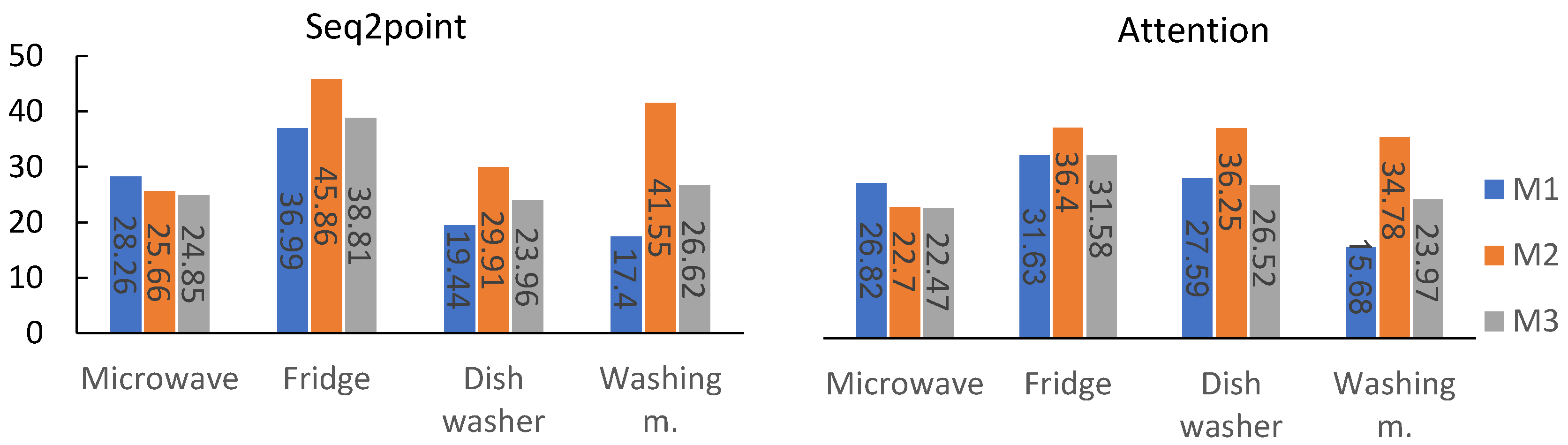
Microwave	28.26	0.1575	26.82	0.0889	25.66	0.2954	22.70	0.2331
Refrigerator	36.99	0.3168	31.63	0.2292	45.86	0.1897	36.40	0.0183
Dishwasher	19.44	0.3139	27.59	0.2565	29.91	0.7898	36.25	0.5370
Washing m.	17.40	0.1073	15.68	0.1204	41.55	0.5924	34.78	0.8437

shows the test results of the two models in the REDD dataset. The effect of predicting with the pretrained model was not good and led to many more test errors for both models. This result indicates that the pattern learned by the model from REFIT is not applicable to the REDD data.

Table 5. Transfer learning from REFIT to UK-DALE.

Appliance	Trained on UK-DALE Test on UK-DALE				Pretrained on REFIT Test on UK-DALE
	Seq2point		Attention		Seq2point		Attention
	MAE	SAE	MAE	SAE	MAE	SAE	MAE	SAE
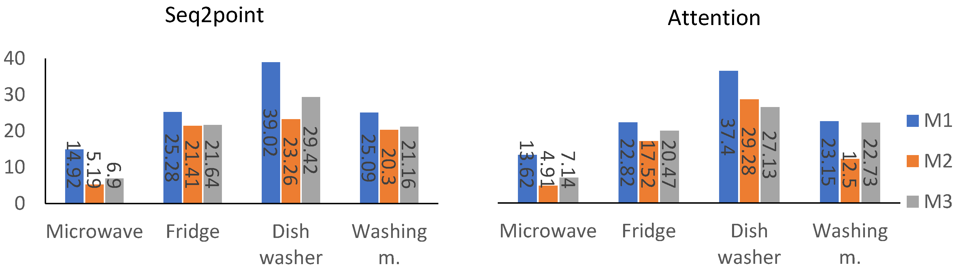
Microwave	14.92	0.5146	13.62	0.4270	5.19	0.0601	4.91	0.0024
Refrigerator	25.28	0.3355	22.82	0.3123	21.41	0.1901	17.52	0.0172
Dishwasher	39.02	0.6837	37.40	0.5075	23.26	0.3515	29.28	0.2647
Washing m.	25.09	0.4881	23.15	0.7655	20.30	0.8073	12.50	0.5829

provides the test results of the two models for the UK-DALE dataset. Using the pretrained model significantly reduced the test errors of the two models, indicating that the pattern learned by the model from REFIT can be applied to UK-DALE. The experimental results of this part support the conclusions about CTL in ref. [22]: due to differences in manufacturing standards, appliances from different countries (REFIT and REDD are from Britain and America, respectively) cannot be directly transferred; appliances in the same country can be directly transferred (both REFIT and UK-DALE come from Britain). The attention model proposed herein performed better than the seq2point model in decomposing the three appliances (except for the dishwasher), and the conclusions before and after transfer are consistent. For the dishwasher, although the seq2point model is better than the attention model according to the MAE, the SAE indicates that the attention model is superior to the seq2point model. Thus, both the MAE and the SAE may have defects as indicators for assessing NILM problems. More effective assessment indicators should be identified in subsequent research.

In the second part of the experiment, the pretrained model was fine-tuned through the training sets UK-DALE and REDD prior to predicting the target data. According to the experience of others, fine-tuning generally only needs to retrain the fully connected layer at the end of the neural network.

Table 6. Transfer learning with fine-tuning dense layers.

Appliance	Pretrained on REFIT Fine-Tuning on REDD				Pretrained on REFIT Fine-Tuning on UK-DALE
	Seq2point		Attention		Seq2point		Attention
	MAE	SAE	MAE	SAE	MAE	SAE	MAE	SAE
Microwave	24.85	0.1685	22.47	0.0499	6.90	0.4921	7.14	0.4042
Refrigerator	38.81	0.0138	31.58	0.1823	21.64	0.2127	20.47	0.2613
Dishwasher	23.96	0.4319	26.52	0.5062	29.42	0.4147	27.13	0.4552
Washing m.	26.62	0.2386	23.97	0.1236	21.16	0.4503	22.73	0.5540

shows the effect of the model on the target test set after fine-tuning the fully connected layer. By comparing Table 4 and Table 5, the fine-tuned model performed much better on REDD, while it performed much worse on UK-DALE. This result also supports the conclusions drawn in ref. [22]: fine-tuning can improve the prediction effects for cross-domain data but cause overfitting for non-cross-domain data.

Figure 4 and Figure 5 present the learning effects of the seq2point model and the attention model for the different datasets. M1 was only trained on the target dataset, M2 was pretrained on REFIT without fine-tuning, and M3 was both pretrained and fine-tuned. Overall, regardless of whether or not transfer learning was conducted, the SAE of the attention model was smaller than that of the seq2point model. For the four types of electric appliances in the experiment, the attention model proposed herein performed better for the microwave, refrigerator, and washing machine than the seq2point model, yet it performed much worse for the dishwasher. This finding may be because this appliance has a complex operating principle so that it is hard for the model to extract the features of its state changes. In addition, it may be related to the data window size selected for training. For example, ref. [31] reduced the data window of the seq2point model from 599 to 100, introduced the short-seq2point model, and demonstrated that the new model can better complete the NILM task. In terms of the transfer ability, the attention model after transfer had a better performance than that without transfer learning on REDD for the three appliances other than the washing machine, while the seq2point model only performed well for the microwave. The results on UK-DALE show that the model after transfer worked much better than that without transfer. With respect to indicator improvement, the attention model was slightly better than the seq2point model, indicating that the new model proposed herein can perfectly solve the NILM problem and is more appropriate for transfer learning.

5. Conclusions

In this paper, a deep neural network model based on an attention mechanism was proposed and applied to NILM transfer learning to decompose a residential power load. This model replaces the traditional RNN by introducing an embedding layer of a time vector (Time2Vector) and then uses an attention layer to obtain a different attention score for each point of the input sequence through training prior to predicting the output. This design utilizes an attention mechanism to improve the traditional seq2seq model, which increases the training speed, enhances the ability of the model to extract signal features, and significantly promotes the accuracy of load decomposition. The experimental results on the three public datasets REFIT, UK-DALE, and REDD show that in most cases, the new model has a better effect than the seq2point model, which is the most commonly used model, especially in terms of its transferability in transfer learning. The conclusion that transfer learning can be applied in NILM was also verified in papers by ref. [22,32]. This result has important practical value, as transfer learning offers a solution when there is a lack of high-quality NILM datasets in the field. Due to space limitations, CTL but not ATL was discussed in this paper; load decomposition only uses low-frequency data and ignores finer-grained signal features, which may lead to the inaccurate prediction of appliance-related events; in the experiment, we showed that the conclusions from the MAE and SAE assessments are inconsistent, which means that assessment indicators that are more applicable to NILM need to be further developed. In addition, smart-home technology is promising to improve NILM technology. For example, smart sockets can record and provide a large number of labelled data to solve insufficient data issues for NILM model training. These issues should be addressed in future research.

References

- Hart, G.W. Nonintrusive Appliance Load Monitoring. Proc. IEEE 1992, 80, 1870–1891. [Google Scholar] [CrossRef]
- Cheng, X.; Li, L.; Wu, H.; Ding, Y.; Song, Y.; Sun, W. A Survey of The Research on Non-intrusive Load Monitoring and Disaggregation. Power Syst. Technol. 2016, 40, 3108–3117. [Google Scholar] [CrossRef]
- Gupta, S.; Reynolds, M.S.; Patel, S.N. ElectriSense:Single-Point Sensing Using EMI for Electrical Event Detection and Classification in the Home. In Proceedings of the 12th ACM International Conference on Ubiquitous Computing; ACM: New York, NY, USA, 2010; pp. 139–148. [Google Scholar] [CrossRef]
- Bouhouras, A.S.; Milioudis, A.N.; Labridis, D.P. Development of Distinct Load Signatures for Higher Efficiency of NILM Algorithms. Electr. Power Syst. Res. 2014, 117, 163–171. [Google Scholar] [CrossRef]
- Leeb, S.B.; Shaw, S.R.; Kirtley, J. Transient Event Detection in Spectral Envelope Estimates for Nonintrusive Load Monitoring. IEEE Trans. Power Deliv. 2014, 10, 1200–1210. [Google Scholar] [CrossRef]
- Medeiros, A.P.; Canha, L.N.; Bertineti, D.P.; de Azevedo, R.M. Event Classification in Non-Intrusive Load Monitoring Using Convolutional Neural Network. In Proceedings of the 2019 IEEE PES Innovative Smart Grid Technologies Conference—Latin America (ISGT Latin America), Gramado, Brazil, 15–18 September 2019; pp. 1–6. [Google Scholar]
- Kim, J.; Le, T.-T.-H.; Kim, H. Nonintrusive Load Monitoring Based on Advanced Deep Learning and Novel Signature. Comput. Intell. Neurosci. 2017, 2017, e4216281. [Google Scholar] [CrossRef]
- Ruano, A.; Hernandez, A.; Ureña, J.; Ruano, M.; Garcia, J. NILM Techniques for Intelligent Home Energy Management and Ambient Assisted Living: A Review. Energies 2019, 12, 2203. [Google Scholar] [CrossRef]
- Pereira, L.; Nunes, N. An Experimental Comparison of Performance Metrics for Event Detection Algorithms in NILM. In Proceedings of the 4th International NILM Workshop, Austin, TX, USA, 7–8 March 2018. [Google Scholar]
- Tan, C.; Sun, F.; Kong, T.; Zhang, W.; Yang, C.; Liu, C. A Survey on Deep Transfer Learning. arXiv 2018, arXiv:1808.01974. [Google Scholar]
- Huang, J.-T.; Li, J.; Yu, D.; Deng, L.; Gong, Y. Cross-Language Knowledge Transfer Using Multilingual Deep Neural Network with Shared Hidden Layers. In Proceedings of the 2013 IEEE International Conference on Acoustics, Speech and Signal Processing, Vancouver, BA, Canada, 26–31 May 2013; pp. 7304–7308. [Google Scholar]
- Yosinski, J.; Clune, J.; Bengio, Y.; Lipson, H. How Transferable Are Features in Deep Neural Networks? arXiv 2014, arXiv:1411.1792. [Google Scholar]
- Devlin, J.; Chang, M.-W.; Lee, K.; Toutanova, K. BERT: Pre-Training of Deep Bidirectional Transformers for Language Understanding. arXiv 2018, arXiv:1810.04805. [Google Scholar]
- Kelly, J.; Knottenbelt, W. Neural NILM:Deep Neural Networks Applied to Energy Disaggregation. In Proceedings of the ACM International Conference on Embedded Systems for Energy-Efficient Built Environments, Seoul, Korea, 4–5 November 2015; pp. 55–64. [Google Scholar]
- Kelly, J.; Knottenbelt, W. The UK-DALE Dataset, Domestic Appliance-Level Electricity Demand and Whole-House Demand from Five UK Homes. Sci. Data 2014, 2, 150007. [Google Scholar] [CrossRef]
- Çavdar, İ.H.; Faryad, V. New Design of a Supervised Energy Disaggregation Model Based on the Deep Neural Network for a Smart Grid. Energies 2019, 12, 1217. [Google Scholar] [CrossRef]
- Xia, M.; Liu, W.; Wang, K.; Zhang, X.; Xu, Y. Non-Intrusive Load Disaggregation Based on Deep Dilated Residual Network. Electr. Power Syst. Res. 2019, 170, 277–285. [Google Scholar] [CrossRef]
- Balduzzi, D.; Frean, M.; Leary, L.; Lewis, J.P.; Ma, K.W.-D.; McWilliams, B. The Shattered Gradients Problem: If Resnets Are the Answer, Then What Is the Question? arXiv 2018, arXiv:1702.08591. [Google Scholar]
- Jiang, J.; Kong, Q.; Plumbley, M.; Gilbert, N. Deep Learning Based Energy Disaggregation and On/Off Detection of Household Appliances. arXiv 2019, arXiv:1908.00941. [Google Scholar]
- Sutskever, I.; Vinyals, O.; Le, Q.V. Sequence to Sequence Learning with Neural Networks. In Proceedings of the Advances in neural information processing systems, Montreal, QC, Canada, 8–13 December 2014; pp. 3104–3112. [Google Scholar]
- Zhang, C.; Zhong, M.; Wang, Z.; Goddard, N.; Sutton, C. Sequence-to-Point Learning with Neural Networks for Nonintrusive Load Monitoring. arXiv 2017, arXiv:1612.09106. [Google Scholar]
- DIncecco, M.; Squartini, S.; Zhong, M. Transfer Learning for Non-Intrusive Load Monitoring. arXiv 2019, arXiv:1902.08835. [Google Scholar] [CrossRef]
- Bahdanau, D.; Cho, K.; Bengio, Y. Neural Machine Translation by Jointly Learning to Align and Translate. arXiv 2014, arXiv:1409.0473. [Google Scholar]
- Luong, M.-T.; Pham, H.; Manning, C.D. Effective Approaches to Attention-Based Neural Machine Translation. arXiv 2015, arXiv:1508.04025. [Google Scholar]
- Cho, K.; Merrienboer, B.V.; Gulcehre, C.; Bougares, F.; Bengio, Y. Learning Phrase Representations Using RNN Encoder-Decoder for Statistical Machine Translation. arXiv 2014, arXiv:1406.1078. [Google Scholar] [CrossRef]
- Kazemi, S.M.; Goel, R.; Eghbali, S.; Ramanan, J.; Sahota, J.; Thakur, S.; Wu, S.; Smyth, C.; Poupart, P.; Brubaker, M. Time2Vec: Learning a Vector Representation of Time. arXiv 2019, arXiv:1907.05321. [Google Scholar]
- Krystalakos, O.; Nalmpantis, C.; Vrakas, D. Sliding Window Approach for Online Energy Disaggregation Using Artificial Neural Networks. In Proceedings of the 10th Hellenic Conference on Artificial Intelligence—SETN ’18; ACM Press: Patras, Greece, 2018; pp. 1–6. [Google Scholar]
- Ebrahim, A.F.; Mohammed, O. Household Load Forecasting Based on a Pre-Processing Non-Intrusive Load Monitoring Techniques. In Proceedings of the 2018 IEEE Green Technologies Conference (GreenTech), Austin, TX, USA, 4–6 April 2018; pp. 107–114. [Google Scholar]
- Kolter, J.Z.; Johnson, M.J. REDD: A Public Data Set for Energy Disaggregation Research. In Proceedings of the Workshop on Data Mining Applications in Sustainability (SIGKDD), San Diego, CA, USA, 21–24 August 2011; Volume 25, pp. 59–62. [Google Scholar]
- Murray, D.; Stankovic, L.; Stankovic, V. An Electrical Load Measurements Dataset of United Kingdom Households from a Two-Year Longitudinal Study. Sci. Data 2017, 4, 160122. [Google Scholar] [CrossRef] [PubMed]
- Zeidi, O.A. Deep Neural Networks for Non-Intrusive Load Monitoring. Master’s Thesis, MONASH University, Melbourne, Australia, 2018. [Google Scholar]
- Zhou, Z.; Xiang, Y.; Xu, H.; Yi, Z.; Shi, D.; Wang, Z. A Novel Transfer Learning-Based Intelligent Nonintrusive Load-Monitoring With Limited Measurements. IEEE Trans. Instrum. Meas. 2021, 70, 1–8. [Google Scholar] [CrossRef]