Article

Bootstrapped Ensemble of Artificial Neural Networks Technique for Quantifying Uncertainty in Prediction of Wind Energy Production

1
Department of Mechanical and Maintenance Engineering, School of Applied Technical Sciences, German Jordanian University, Amman 11180, Jordan
2
Energy Department, Politecnico di Milano, Via La Masa 34, 20156 Milan, Italy
3
MINES ParisTech, PSL Research University, CRC, 06560 Sophia Antipolis, France
4
Department of Nuclear Engineering, Eminent Scholar, College of Engineering, Kyung Hee University, Seoul 130-701, Korea
5
Research Development and Innovation, Edison Spa, Foro Buonaparte 31, 20121 Milan, Italy
*
Author to whom correspondence should be addressed.
Sustainability 2021, 13(11), 6417; https://doi.org/10.3390/su13116417
Submission received: 1 May 2021 / Revised: 27 May 2021 / Accepted: 3 June 2021 / Published: 4 June 2021

Abstract

:
The accurate prediction of wind energy production is crucial for an affordable and reliable power supply to consumers. Prediction models are used as decision-aid tools for electric grid operators to dynamically balance the energy production provided by a pool of diverse sources in the energy mix. However, different sources of uncertainty affect the predictions, providing the decision-makers with non-accurate and possibly misleading information for grid operation. In this regard, this work aims to quantify the possible sources of uncertainty that affect the predictions of wind energy production provided by an ensemble of Artificial Neural Network (ANN) models. The proposed Bootstrap (BS) technique for uncertainty quantification relies on estimating Prediction Intervals (PIs) for a predefined confidence level. The capability of the proposed BS technique is verified, considering a 34 MW wind plant located in Italy. The obtained results show that the BS technique provides a more satisfactory quantification of the uncertainty of wind energy predictions than that of a technique adopted by the wind plant owner and the Mean-Variance Estimation (MVE) technique of literature. The PIs obtained by the BS technique are also analyzed in terms of different weather conditions experienced by the wind plant and time horizons of prediction.

1. Introduction

The contribution of wind energy to the electricity production portfolio is increasing compared to other productions with energy sources, such as nuclear, coal, hydroelectric, oil and gas, and biomass plants [1,2]. Wind energy production capacity grew by more than 18% (111 GW) in 2020, for an overall capacity of 733 GW [3]. In some EU countries, wind has become the mainstream source of electricity production, e.g., in Denmark, where it constitutes 48% of the country’s total electricity consumption in 2020 followed by Ireland (38%), Portugal (25%), Germany (27%), and the UK (27%) [4].
A difficulty for wind energy production comes from the wind speed fluctuations, leading to large uncertainties in wind energy productions [5,6,7,8,9,10,11].
Different prediction models have been developed and used to estimate energy productions in wind plants. Generally, we can distinguish model-based and data-driven approaches [12,13,14]. Model-based approaches employ physics models that utilize wind-forecasting data for wind energy predictions [8,15,16,17]. Data-driven approaches do not use explicit physical models. Instead, they rely exclusively on wind data to build (black-box) models that capture the relationship of wind-forecasting data and the corresponding wind energy productions [7,18,19,20,21].
Over the last few decades, various data-driven methods have been widely developed and applied with success to wind energy prediction. A few that are worth mentioning include, Artificial Neural Networks (ANNs) [22,23,24,25]; Support Vector Machines (SVMs) [10,17,23,26,27]; k-nearest neighbors (k-nn) regression [24,28,29]; Support Vector Regression (SVR) [8]; Gaussian Process Regression (GPR) [23,30]. In this work, we consider the use of ANNs given their capability of solving highly non-linear problems in many industrial fields. For example, Mellit and Kalogirou [31] applied ANNs and other AI techniques to different tasks related to the design and operation of photovoltaic systems; Luchetta et al. [32] developed an approach for fault detection and diagnostics based on ANNs and applied it to Pulse Width Modulated (PWM) DC–DC power converters; De Leon-Aldaco et al. [33] presented a comprehensive review of metaheuristic methodologies in the area of power converters and considered the use of ANNs for modeling the system behavior within the search, to reduce the computational time. ANNs have been already successfully applied in [23,34] for energy production prediction. Ensemble approaches, based on the aggregation of multiple model outcomes, have been shown to be superior to any individual models in the ensemble to enhance the accuracy of the predictions and quantifying their uncertainty [34,35,36]. For example, Zameer et al. [37] proposed a genetic programming-based ensemble of ANNs approach for short-term wind power prediction. The efficacy of the proposed approach was shown with respect to recent artificial intelligence-based strategies on real datasets taken from five different wind farms located in Europe. Al-Dahidi et al. [38] proposed an ensemble of ANNs for wind plant energy production. Specifically, in [38], different strategies used to aggregate the outcomes of the base (individual) models of the ensemble have been investigated and compared on a real dataset taken from a wind plant located in Italy. Lee et al. [36] proposed three ensemble learning-based models (Boosted Trees (BT), Random Forest (RF), and Generalized Random Forest (GRF)) for a reliable short-term wind power prediction. The efficacy of the proposed ensembles was compared to ensembles of different configurations of the GPR and SVR models concerning wind farms located in France and Turkey.
Independently from the choice of the prediction model and of the scheme adopted to provide the final predictions (that can be either individual or ensemble), different sources of uncertainty affect the predictions, providing the decision-makers with non-accurate, and possibly misleading, information for grid operation [37,39,40].
The work presented in this paper focuses on the quantification of the uncertainty of wind energy predictions provided by an ensemble of data-driven models. This is a fundamental task for the management of wind farms, since it allows for informing decision-makers of the possible mismatch between the predicted and the real energy production, and, therefore, to properly evaluate the risk associated with their decisions in critical tasks, such as electric grid management and formulation of energy bidding strategies [41,42,43,44]. In particular, we consider the following sources of uncertainty: (1) uncertainty of the ensemble input (weather forecasts), (2) uncertainty due to the stochastic variability of the physical process, and (3) uncertainty inherent to the prediction model structure and parameters. The objective is the quantification of the overall uncertainty, which affects the predictions provided by the ensemble. Various ANN-based methods have been developed and applied for the estimation of Prediction Intervals (PIs) of energy production predictions, such as Delta [45,46], Bootstrap (BS) [47,48,49,50], Lower Upper Bound Estimation (LUBE) [51,52,53,54], and Mean-Variance Estimation (MVE) [55,56]. For example, Khosravi et al. [56] proposed an optimized MVE method for quantifying the uncertainty associated with the wind power predictions by constructing reliable PIs. The estimated PIs were more informative than those obtained by the traditional MVE method for three wind farms located in Australia. Wen et al. [52] proposed a novel method based on LUBE for predicting wind power production and quantifying the associated uncertainty in both hourly and daily modes. The quality of the estimated PIs obtained by the proposed method was superior to other PIs obtained by other benchmarks for different wind farms located in Taiwan. Quan et al. [54] proposed a Particle Swarm Optimization (PSO)-based LUBE method for short-term load and wind power prediction and uncertainty quantification. The quality of the constructed PIs was superior to other PIs obtained by other benchmarks for the load and wind power production prediction in a short time.
In this work, the BS technique is considered. It has already been applied and shown to be effective for quantifying uncertainty in different industrial applications [41,47,49,57,58]. The PIs are obtained for a predefined confidence level α% [41], i.e., upper and lower bounds of the prediction that bracket the true/actual energy production value with probability α% [59].
Thus, in this work, an ensemble of ANN models is developed for energy production prediction, and the BS is used to quantify the uncertainties that affect the predictions.
BS is applied to a real case study of a wind plant located in the south of Italy with a capacity of 34 MW. For comparison, the technique (hereafter called the Quantile technique) adopted by the wind plant owner for computing the 10th and 90th percentiles of the predictions and the MVE technique of literature are considered. The application results show that BS is superior and more informative for the electric grid decision-makers than Quantile and MVE techniques.
The PIs obtained by the BS are also analyzed in terms of (i) the different operational conditions experienced by the wind plant (i.e., the weather conditions) and (ii) the time horizons (i.e., delays) of the predictions.
With respect to (i), the different weather conditions experienced by the wind plant are identified by resorting to Principal Component Analysis (PCA) [60,61] and Fuzzy C-Means (FCM) [62,63]. The former is used to reduce the dimensionality of the input weather-forecasting data, keeping the relevant information content. In practice, the F weather-forecasting quantities are projected into the space of F* < F principal components, which allow for describing a large fraction of the data variability using few features. The FCM algorithm receives, as an input, the identified F* principal components of the historical dataset and provides output clusters made by data characterized by similar weather conditions. The optimal number of clusters is identified by using the Davies–Bouldin (DB) validity index [64].
Once the different weather conditions are identified, the quality of the PIs obtained by the BS is quantified for each weather condition in terms of PI widths and PI coverage values.
With respect to (ii), the quality of the PIs obtained by the BS is evaluated for each day-ahead production prediction (i.e., until four days ahead) in terms of the Root Mean Square Error (RMSE) used for assessing the accuracy of the production predictions, and the widths of the corresponding PIs at each prediction hour.
The analysis shows that the PIs significantly vary due to the effects of the weather conditions and the time horizon of the predictions.
Thus, the significant contributions of this work are:
  • The quantification of the uncertainty affecting the wind energy production predictions provided by an ensemble of ANNs models employing BS technique;
  • The comparisons with the Quantile (adopted by the plant owner) and MVE (from the literature) techniques used for the uncertainty quantification;
  • The analysis of the BS’s PIs in terms of various influencing factors, such as the different weather conditions experienced by the wind plant and the time horizons of the predictions.
The remainder of this paper is organized as follows. In Section 2, the ensemble of ANN models for predicting wind energy production is presented. In Section 3, the BS technique for constructing PIs is described. In Section 4, the results of applying the BS technique to a real case study of a wind plant are presented and compared with those obtained by the Quantile approach of the wind plant owners and the MVE technique in the literature. In Section 5, the PIs obtained by the BS technique are analyzed with respect to the different operational conditions experienced by the wind plant and the time horizons of the predictions. Finally, some conclusions are drawn in Section 6.

2. Ensemble Approach for the Prediction of Energy Production in Wind Plants

In this Section, the ensemble approach for predicting energy production is described.
Ensemble approaches have been applied in various application fields to enhance the accuracy of the predictions and quantify their uncertainty [34,35]. The basic idea is that the individual models of the ensemble can complement each other by leveraging their strengths and overcoming their drawbacks: thus, the aggregation of their outcomes can boost the performance of the models [35,65,66,67].
A typical ensemble of models for energy production prediction is shown in Figure 1. A training dataset X t r a i n , which comprises the weather-forecasting data ( W F ) and the associated energy productions ( P ), is utilized for building the individual models of the ensemble (hereafter called the base models). Once constructed, the ensemble provides the prediction of the energy production ( P ^ e n s e m b l e ) for any new coming test pattern, whose input weather-forecasting data W F j t e s t at time t j is provided by a weather-forecast model. For this, the ensemble performs two steps [35,66]: (1) energy production predictions by the individual prediction models, and (2) aggregation of the energy production predictions.
Correspondingly, the two key components for constructing an effective ensemble approach are [35,66,68]: (1) a strategy for obtaining diversity among the H base models and (2) a strategy for aggregating the H outcomes of the base models.
With respect to (1), different strategies have been developed for injecting the diversity among the base models of the ensemble, e.g., adopting different predictive modeling techniques, adopting the same prediction model type but with different parameter settings, and training each model with different training datasets, by resorting to techniques such as Bootstrapping AGGregatING (BAGGING) [69,70], Boosting [71], and Adaboost [72]. The reader interested in more details on the techniques used for generating diversity in the base models can refer to [69].
In this work, we use BAGGING to create the H diverse base models of the ensemble. The basic idea of BAGGING is to train the base models with different training datasets generated by bootstrap [73]: the different versions of the training datasets are created by randomly sampling from the original training dataset X t r a i n with replacement.
Artificial Neural Network (ANN) is employed as a base model for the prediction of energy production. The motivation for using an ensemble of ANNs is the fact that this model is currently used by some energy production companies for wind energy production prediction, and it has been shown capable of providing more accurate and robust predictions than individual models [38].
With respect to (2), different strategies have been proposed for an effective aggregation of the base models’ outcomes into a final aggregated one, e.g., statistics-based (Simple Average (SA) and Simple Median (SM)), and model performance-based (Globally Weighted Average (GWA) and Locally Weighted Average (LWA) (Local Fusion (LF))) [35,74,75].
In practice, the aggregation of the base model outcomes entails (1) assuming a weight w h for the energy production prediction P ^ h obtained by each base model h ,   h = 1 , , H , and (2) aggregating the H outcomes as a weighted average:
P ^ e n s e m b l e = h = 1 H w h . P ^ h h = 1 H w h ,   h = 1 , , H
SA weights all the outcomes of the base models with equal weights, i.e., w h = 1 H . SM takes only the center value of the H base model outcomes distribution, i.e., it assumes that the weights are all equal to 0 except for that corresponding to the median of the H base model outcomes. GWA and LWA consider weights for the base models that are inversely proportional to their prediction performance computed on a validation dataset and neighboring validation patterns close to the test pattern under study, respectively.

3. PIs for Uncertainty Quantification of Wind Production Prediction

A PI with confidence level α % is defined as an interval [ P ^ j l o w e r , P ^ j u p p e r ] , such that the probability that the true/actual energy production value, P j , of the test pattern at the time t j falls within the interval is equal to α % [41,59]:
P I α = [ P ^ j l o w e r , P ^ j u p p e r ] : P r o b ( P ^ j l o w e r P j P ^ j u p p e r ) = α
For evaluating the estimated PIs, two indicators are considered: (i) the coverage, i.e., the fraction of the true/actual energy productions which actually fall within the constructed PIs, and (ii) the PIs width. A PI with confidence α % should have coverage of at least α %, with a width that is as small as possible [41,59,76].

3.1. Bootstrap (BS) Technique

In wind energy predictions, the prediction error variance, σ ε 2 , can be decomposed into three terms corresponding to the following three sources of uncertainty:
  • σ W F 2 is the variance caused by the model input uncertainty, i.e., the weather-forecast errors (source of uncertainty 1);
  • σ P R 2 is the variance caused by the stochastic variability of the physical process (source of uncertainty 2);
  • σ M O 2 is the variance caused by the ensemble model error, e.g., due to random initialization of the ANNs parameters or to the different datasets used for training the ANNs (source of uncertainty 3).
The prediction error variance, σ ε 2 , can be decomposed into the three contributions by:
v a r [ ε ] = σ ε 2 = σ W F 2 + σ P R 2 + σ M O 2
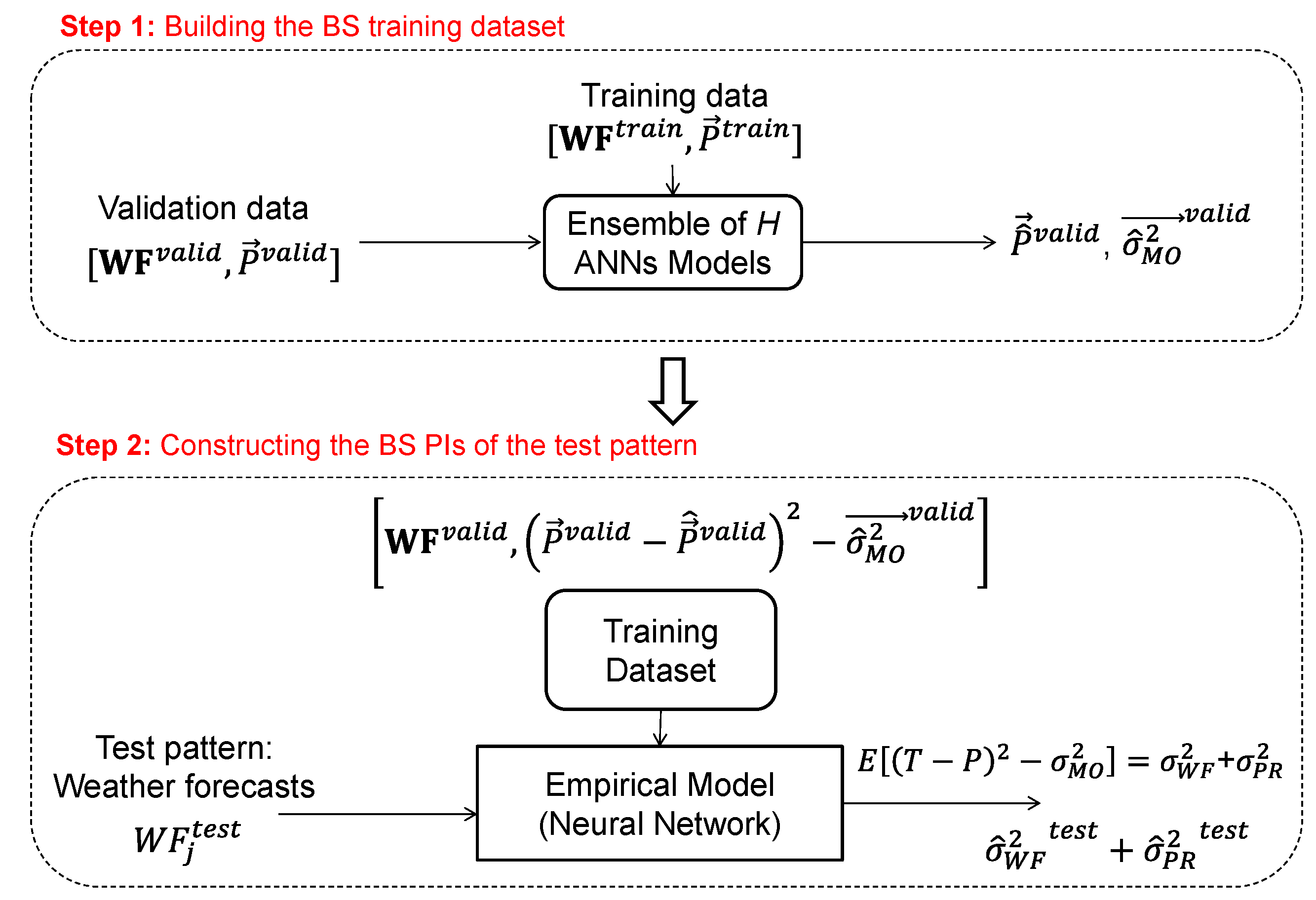
The flowchart of the BS technique for the estimation of the unknown σ ε 2 , and the associated PIs, is sketched in Figure 2. There are three steps:
Step 1: Building the BS training dataset. Let us assume that we have available a dataset of weather-forecasting data and their associated energy productions, X a l l = [ W F a l l , P a l l ] . This dataset is portioned into two datasets: a training dataset X t r a i n = [ W F t r a i n , P t r a i n ] for building the ensemble of ANN models and a validation dataset X v a l i d = [ W F v a l i d , P v a l i d ] for providing estimates of the energy productions, P ^ v a l i d , whose true/actual productions P v a l i d are already known. The variance σ M O 2 v a l i d caused by the ensemble model uncertainty, can then be estimated using X v a l i d :
σ M O 2 v a l i d = v a r ( P ^ v a l i d )
Step 2: Constructing the BS PIs of the test pattern. The BS training dataset X B S t r a i n = [ W F v a l i d , ( P v a l i d P ^ v a l i d ) 2 σ M O 2 v a l i d   ] formed by the weather-forecasting data of the validation dataset, W F v a l i d , and the squared prediction errors of the ensemble on the energy productions of the validation dataset, ( P v a l i d P ^ v a l i d ) 2 σ M O 2 v a l i d is built. Notice that ( P v a l i d P ^ v a l i d ) 2 σ M O 2 v a l i d contains the contributions to the overall error σ ε 2 caused by sources of uncertainty 1 and 2.
With the BS training dataset, X B S t r a i n , a dedicated feedforward ANN is trained. Given a generic test pattern, W F j t e s t , it estimates its corresponding σ W F 2 j t e s t + σ P R 2 j t e s t = σ ε 2 j t e s t σ M O 2 j t e s t .
Finally, the PI of the test pattern at a time t j with a confidence level equal to α % is [55,57]:
[ P ^ j l o w e r , P ^ j u p p e r ] = P ^ j t e s t ± C d o f α . σ ε 2 j t e s t
where P ^ j t e s t is the energy production predicted by the ANN ensemble for the test pattern at a time t j and C d o f α is the ( 1 α ) / 2 quantile of Student t-distribution with a number of degrees of freedom equal to the number of ensemble models H .

4. Case Study

In this section, the ensemble approach of Section 2 is applied to the estimation of the uncertainty affecting the prediction of wind energy productions based on available weather-forecasting data and corresponding known energy productions of a wind plant located in the south of Italy [38] (Section 4.1). The quantification of the three sources of uncertainty (namely, uncertainty due to the model input (weather forecasts), uncertainty due to the inherent variability (stochasticity) of the physical process, and uncertainty due to the model error) is carried out by the BS technique, described in Section 3.1, and the results are compared with those obtained by the technique adopted by the plant owner for the estimation of PIs and the Mean-Variance Estimation (MVE) technique of literature (Section 4.2).

4.1. Data Description and Ensemble Model Development

In this Section, the dataset of real weather-forecasting data, W F , and corresponding energy productions, P , of a wind plant with 34 MW capacity is described. The dataset has been collected every three-hours over three years (from 2011 to 2013) with a forecast horizon Δ t = 96 h (four-day ahead). In other words, at a given time t , the weather-forecasting data of the following Δ t = 96 h are available, with a datum every 3 h, i.e., at time t ,   t + 3   h ,   t + 6   h ,   ,   t + 96   h [38].
Engineering and expert judgment have been used to select a set of F = 19 features (whose detailed characteristics cannot be revealed, due to confidentiality reasons), e.g., wind speeds (in meters/second), horizontal (u) and vertical (v) wind components, hour which the weather forecasting is referred to, temperature, etc., for building the ensemble and predicting the energy productions. Note that for confidentiality reasons, throughout the paper, the values of the wind speeds and energy productions reported in Figures and Table are given on an arbitrary scale.
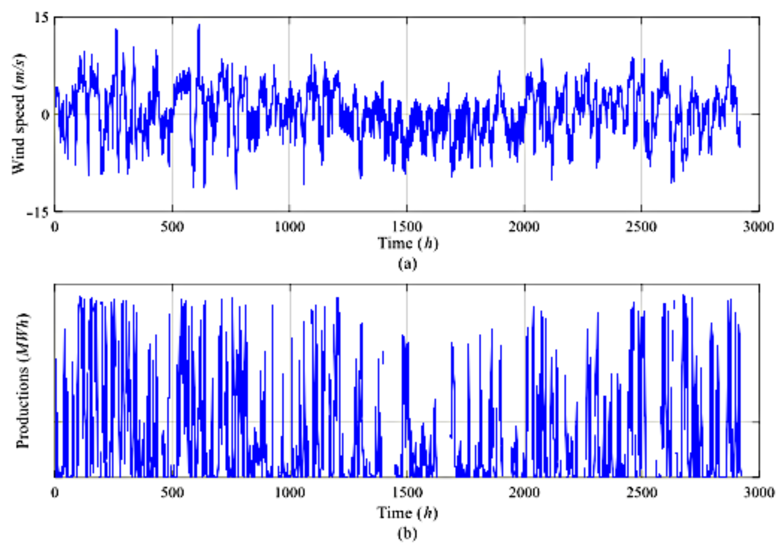
Figure 3 presents the one-day ahead wind speed forecasts (Figure 3a) and corresponding energy productions (Figure 3b) of the year 2013. Figure 3 shows the large variability in the plant’s wind speed and the related large variability of the energy productions. Note that the wind speed sign (i.e., positive or negative) refers to the wind direction. For example, the negative wind speed values of the horizontal component (u) indicate that the direction of the wind is from west to east, whereas the negative wind speed values of the vertical component (v) indicate that the direction of the wind is from north to south.
The data are appended in the matrix X a l l , where rows and columns represent the forecasting patterns and the physical quantities of the weather forecasts with corresponding energy productions, respectively. The 2011–2012 data are divided randomly into X t r a i n training dataset (a fraction of 70% with N t r a i n patterns) and X v a l i d validation dataset (remaining fraction of 30% with N v a l i d patterns) to build the individual models and develop the ensemble, respectively. The 2013 data are used as a test dataset X t e s t .
In this work, an ensemble composed of H = 100 ANNs models has been built. Each ANN is characterized by an architecture with four layers (one input, two hidden, and one output) and 9 × 7 hidden neurons, following a trials-and-errors procedure.
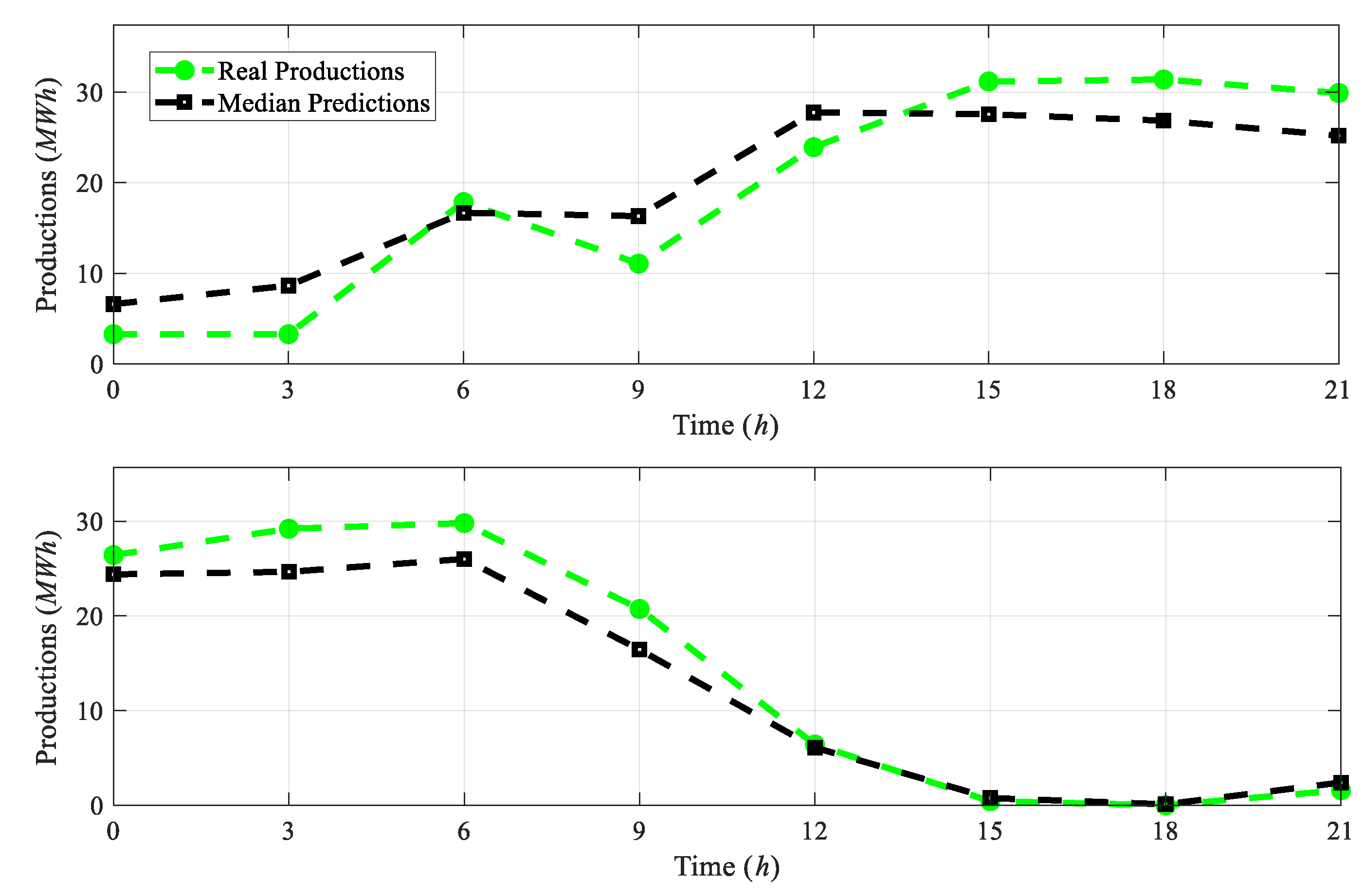
Figure 4 shows two examples of energy production predictions (squares) and the corresponding true values (circles) for two different days of the year 2013. It can be seen that the estimated productions are reasonably close to the actual production values, although in some cases, the prediction error is not negligible (e.g., t = 6 h).

4.2. Application Results of the BS PIs Estimation Technique

In this Section, the PIs obtained by the BS technique on the test data of the year 2013, X t e s t , are presented and compared with those obtained by two other PIs estimation techniques: (1) the technique adopted by the wind plant owner (hereafter called the Quantile technique) and (2) the Mean-Variance Estimation (MVE) technique from the literature.
Briefly, the basic idea of the Quantile technique is to consider the quantiles of the predicted energy productions obtained by the H ANN models of the ensemble of Section 2 at each time t j . The PIs obtained by the Quantile technique are made of the 10th and 90th percentiles (lower and upper bounds, respectively) of the energy production predictions obtained by the H = 100 models of the ensemble, for a target confidence level α   = 80%.
With respect to the MVE technique, its basic idea is to assume that the prediction error obtained by the ensemble, i.e., ε = P P ^ , is an uncertain variable distributed according to a Gaussian distribution function whose variance σ ε 2 has to be estimated by using a dedicated ANN, adequately developed with a procedure similar to that carried out for the BS technique [55]. The dependence of this variance on the weather-forecasting data’s input patterns is the fundamental assumption of the MVE (refer to Appendix A for more details on the MVE technique for PIs estimation [55]).
For each of the BS and the MVE techniques, a dedicated feedforward ANN, with an architecture of three layers (input, hidden, and output) and seven hidden neurons, is developed to estimate the prediction error variance with the BS and MVE techniques.
Table 1 reports the application results of the three PIs estimation techniques. Looking at Table 1, one can notice the following:
  • The PIs obtained by the Quantile technique are narrow (i.e., 4.625) but have very low coverage values (i.e., 0.3352);
  • The MVE technique provides wider PIs (i.e., 11.67) than the Quantile technique (i.e., 4.625), with consequent larger coverage probability (i.e., 0.6534 vs. 0.3352, respectively). Still, it does not achieve the coverage level of 0.8;
  • The BS technique is superior to the Quantile and MVE techniques: although it provides wider PIs than the Quantile technique and slightly wider PIs than the MVE technique, it allows for obtaining a coverage larger than 0.8 (i.e., 0.81).
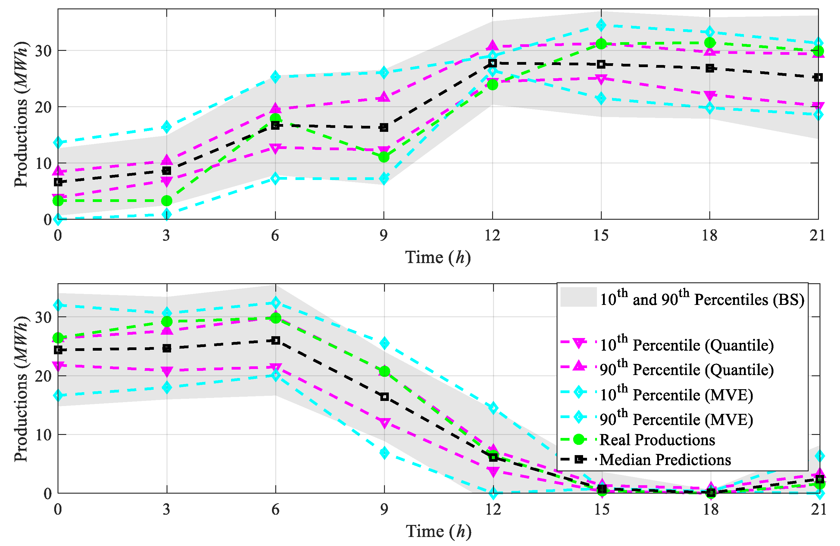
For illustration purposes, the energy production predictions (squares) and the true production values (circles) together with the PIs obtained by the BS (shaded area), Quantile (triangles), and MVE (diamonds) techniques for two different days of the year 2013 test data are shown in Figure 5. It can be seen that:
  • The PIs obtained by the Quantile technique (triangles) are narrow but with very low coverage values, i.e., the actuals productions fall outside the estimated PIs;
  • The PIs obtained by the MVE technique (diamonds) are wider than the PIs of the Quantile technique, and, consequently, have larger PI coverage probabilities;
  • The PIs obtained by the BS technique (shaded area) are wider than the Quantile technique (triangles) and slightly wider than the MVE technique (diamonds), and, consequently, the BS PIs have larger PI coverage probabilities, i.e., the true productions fall inside the estimated BS PIs.

5. Factors Influencing the Estimated BS PIs

In this section, the PIs obtained by the BS technique are analyzed in terms of (i) the different weather conditions that influence the wind energy productions (Section 5.1) and (ii) the time horizons (i.e., delays) of the predictions (Section 5.2).

5.1. Influence of the Weather Conditions

The wind plant under study is, indeed, affected by a very large variability in the weather conditions (Figure 3). In practice, one might be interested in (1) identifying the different weather conditions that can be experienced by the plant, e.g., low, medium, and high wind speed values, based on the available weather-forecasting data, and consequently, (2) investigating their influence on the estimated BS PIs.
With respect to (1), the overall dataset, X a l l , has been further analyzed as follows:
  • The dataset is high dimensional, i.e., it comprises F = 19 physical quantities of the weather forecasts and, therefore, it has been transformed into F * fewer dimensions by resorting to Principal Component Analysis (PCA) [60,61].
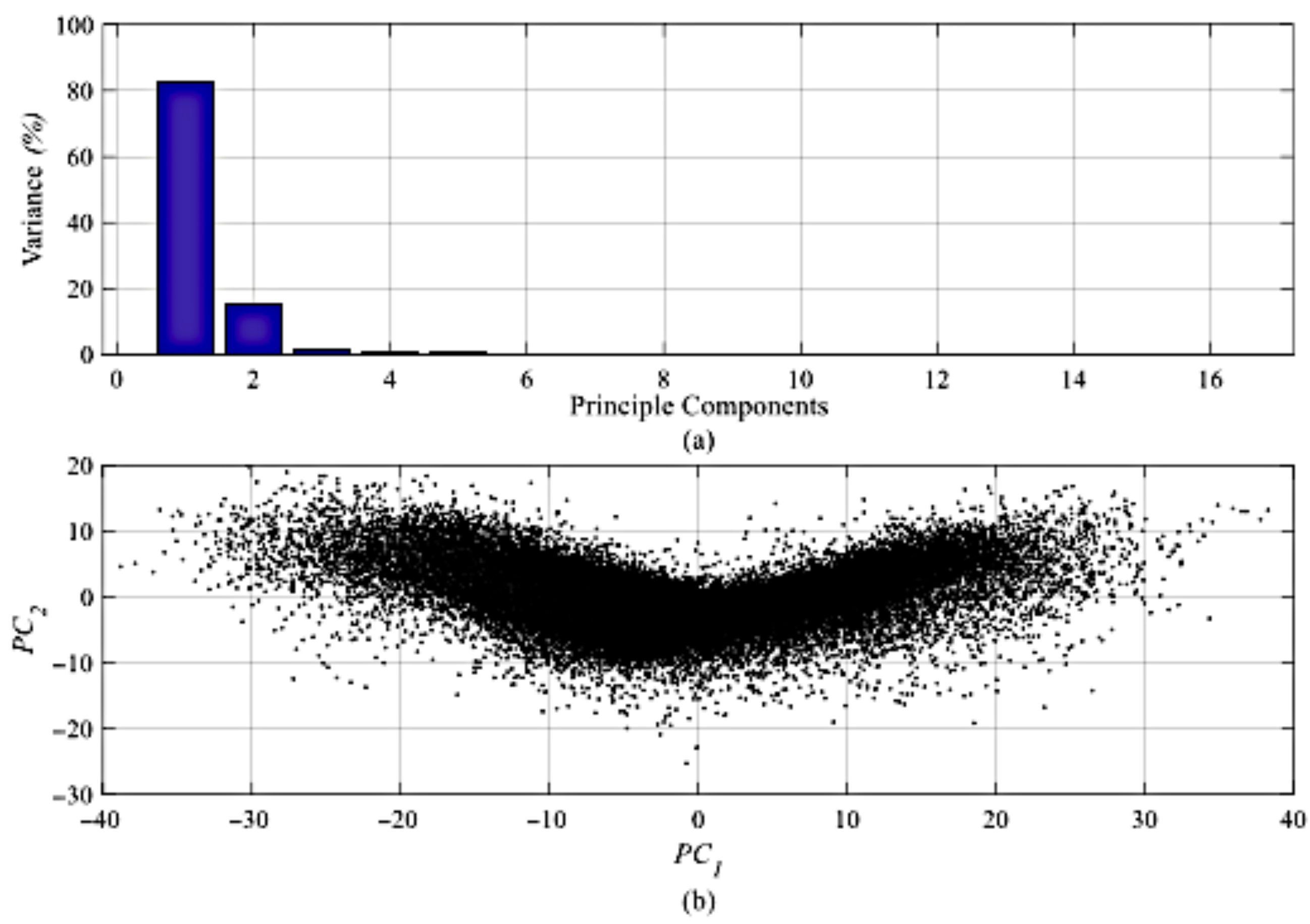
Two principal components, F * = 2 , have been selected as representative of the weather forecast data of the wind plant under study. Figure 6a shows that the selected PCs explain 97% of the original weather forecast data, whereas Figure 6b shows the overall dataset in the space of the identified principal components.
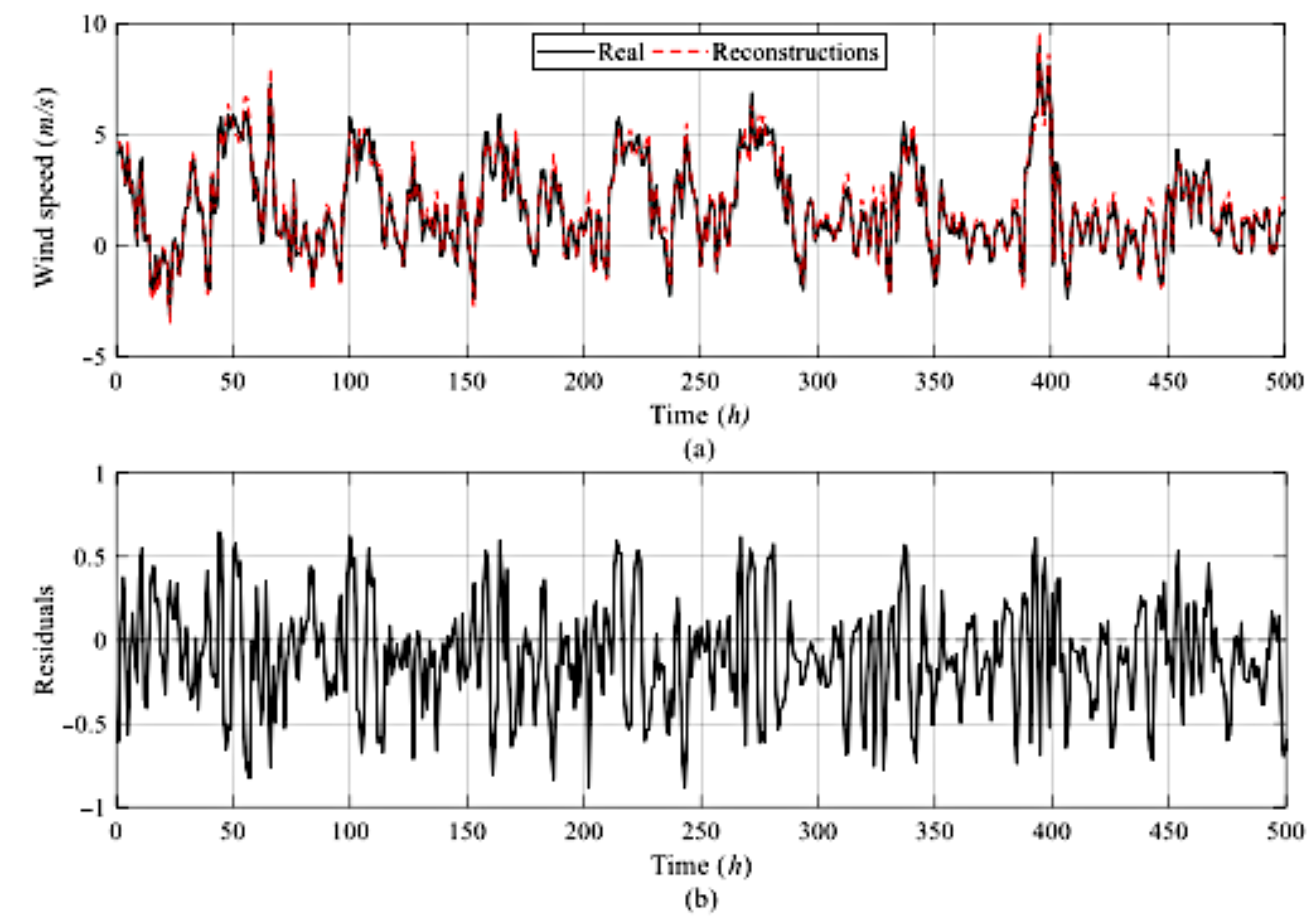
The two selected principal components can describe the dataset with reasonable accuracy: indeed, Figure 7a shows that the two components are capable of reconstructing the original weather forecast data (for the sake of clarity, the first 500 h are plotted) with low reconstruction errors, i.e., with residuals close to 0 (Figure 7b).
  • In the space of the identified principal components, the dataset has been partitioned into S dissimilar groups (whose number is “a priori” unknown), such that data belonging to the same group are very similar to each other and dissimilar to those of the other groups. The S groups can be interpreted as different operating conditions of the wind plant that can influence the wind energy production.
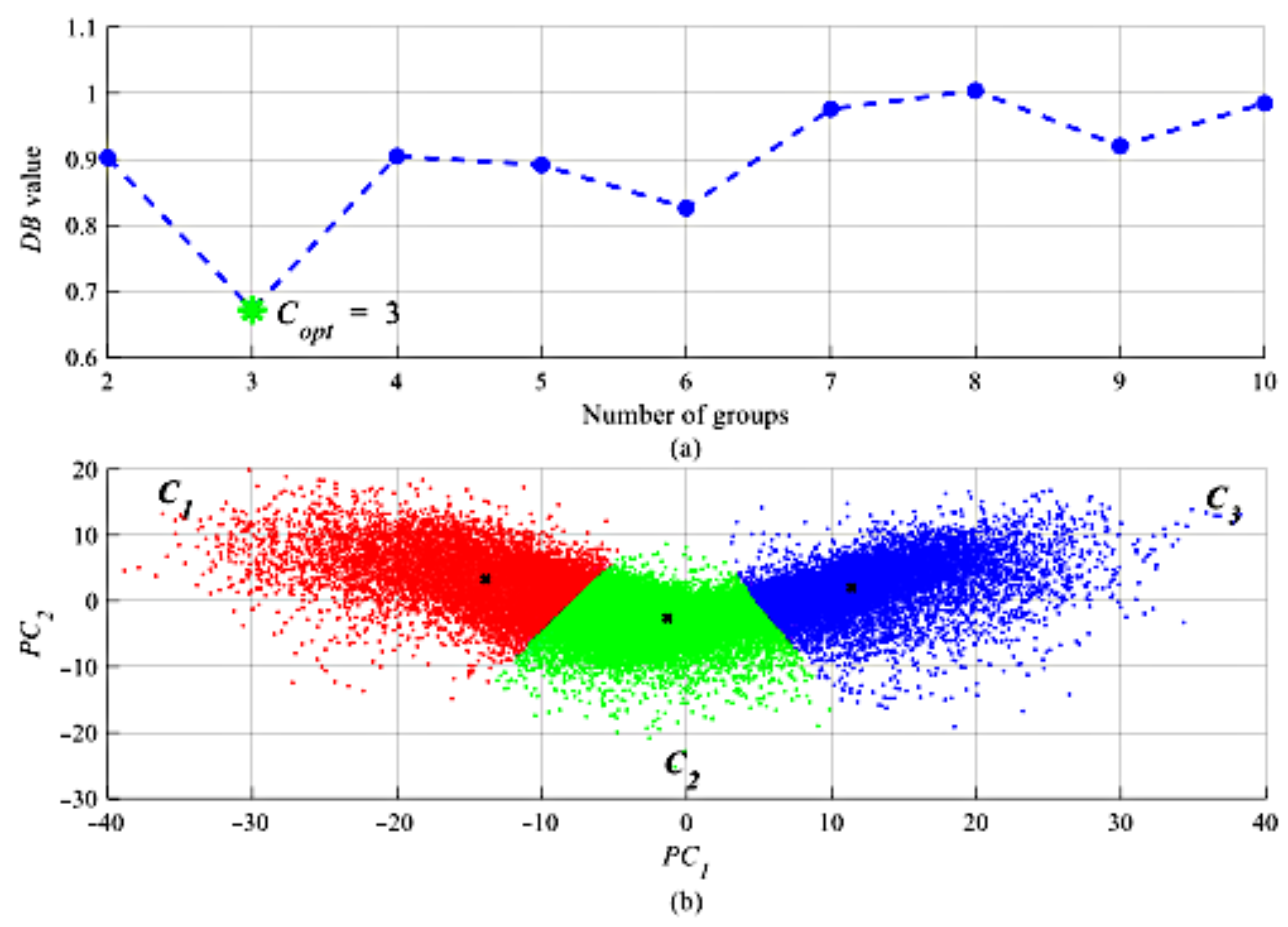
To this aim, the data shown in Figure 6b are clustered by the unsupervised Fuzzy C-Means (FCM) algorithm [62,63]. For identifying the optimum number of the groups C o p t , single clustering validity index (e.g., Silhouette, Davies–Bouldin (DB), etc.) or a combination of different validity indices can be used [77]. In this work, Davies–Bouldin (DB) validity criterion has been considered for clustering the groups of the dataset of Figure 6b. The Davies–Bouldin (DB) criterion is based on the ratio of within-group and between-group distances: the optimal partition, which gives optimal separation and compactness of the obtained groups, has the smallest DB index value [64].
Figure 8a shows the DB values for different numbers of groups in the range of [2,10]: the star indicates the optimum number of groups C o p t . The obtained groups (Figure 8b) correspond to situations of neutral u and negative v components of the wind (operating condition 1), neutral u and v components of the wind (operating condition 2), and positive u and v components of the wind (operating condition 3).
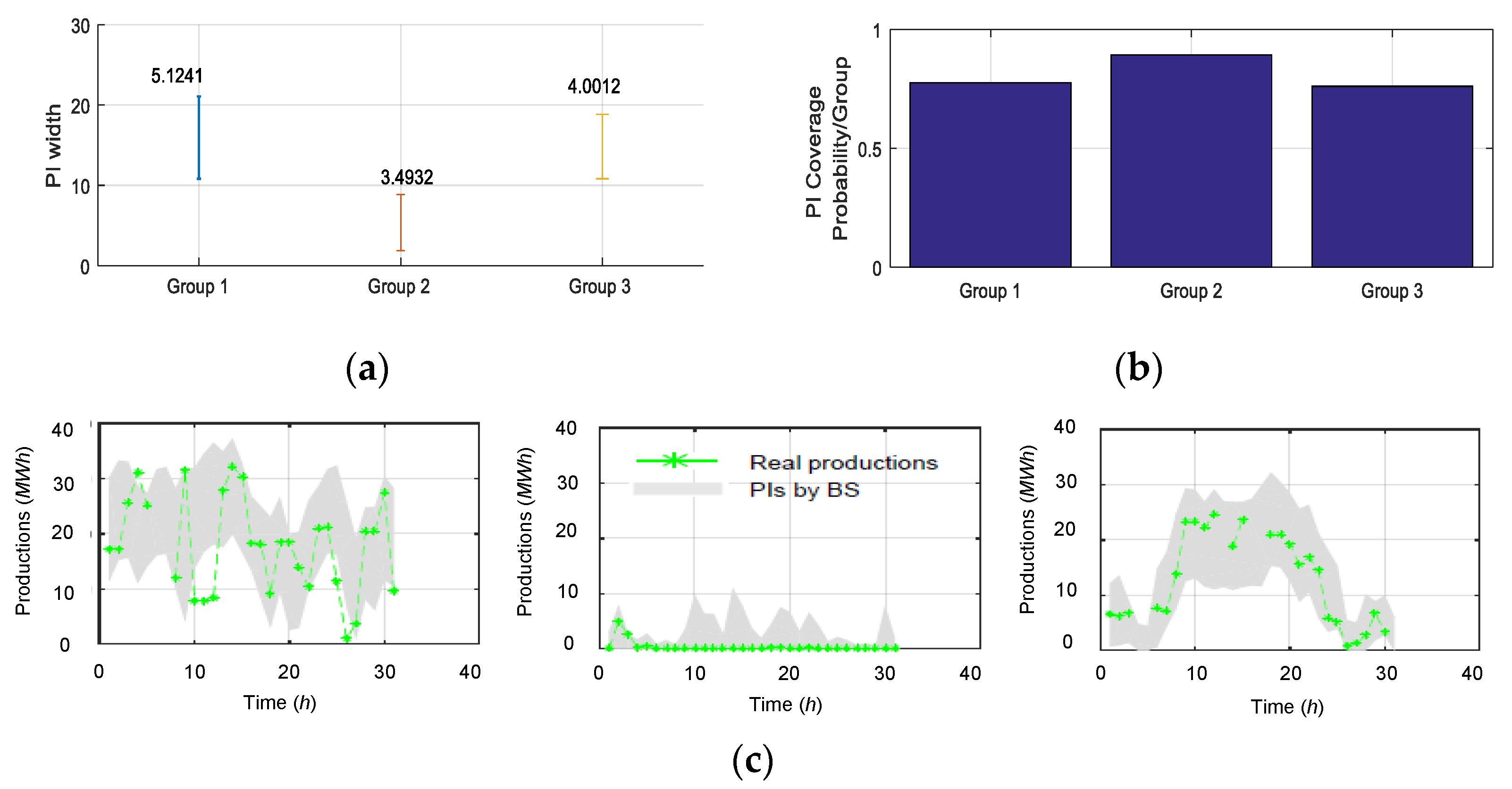
With respect to (2), once the energy production predictions of the 2013 test data are obtained by the ensemble approach of Section 2, the corresponding PIs are estimated by the BS technique of Section 3.1 for the quantification of the uncertainties that affect the predictions. The estimated PIs are evaluated in terms of the three operating conditions of Figure 8b. Figure 9 shows the average PI widths (Figure 9a) and the average PI coverage values (Figure 9b) of the data of the three weather forecast groups. One can easily recognize that the larger the variability of the wind speeds (group 1 and group 3), the larger the prediction error, and, coherently, the larger the width of the PI (the values are indicated on Figure), but the smaller the PI coverage probability, and vice versa.
This can be explained by the fact that the larger the variability of the weather conditions (group 1 and group 3), the larger the wind energy production and, hence, the larger the uncertainty in the energy production prediction, as shown in Figure 9. For clarification purposes, Figure 9c shows examples of the estimated PIs of few data points of the three weather conditions.

5.2. Influence of the Time Horizon

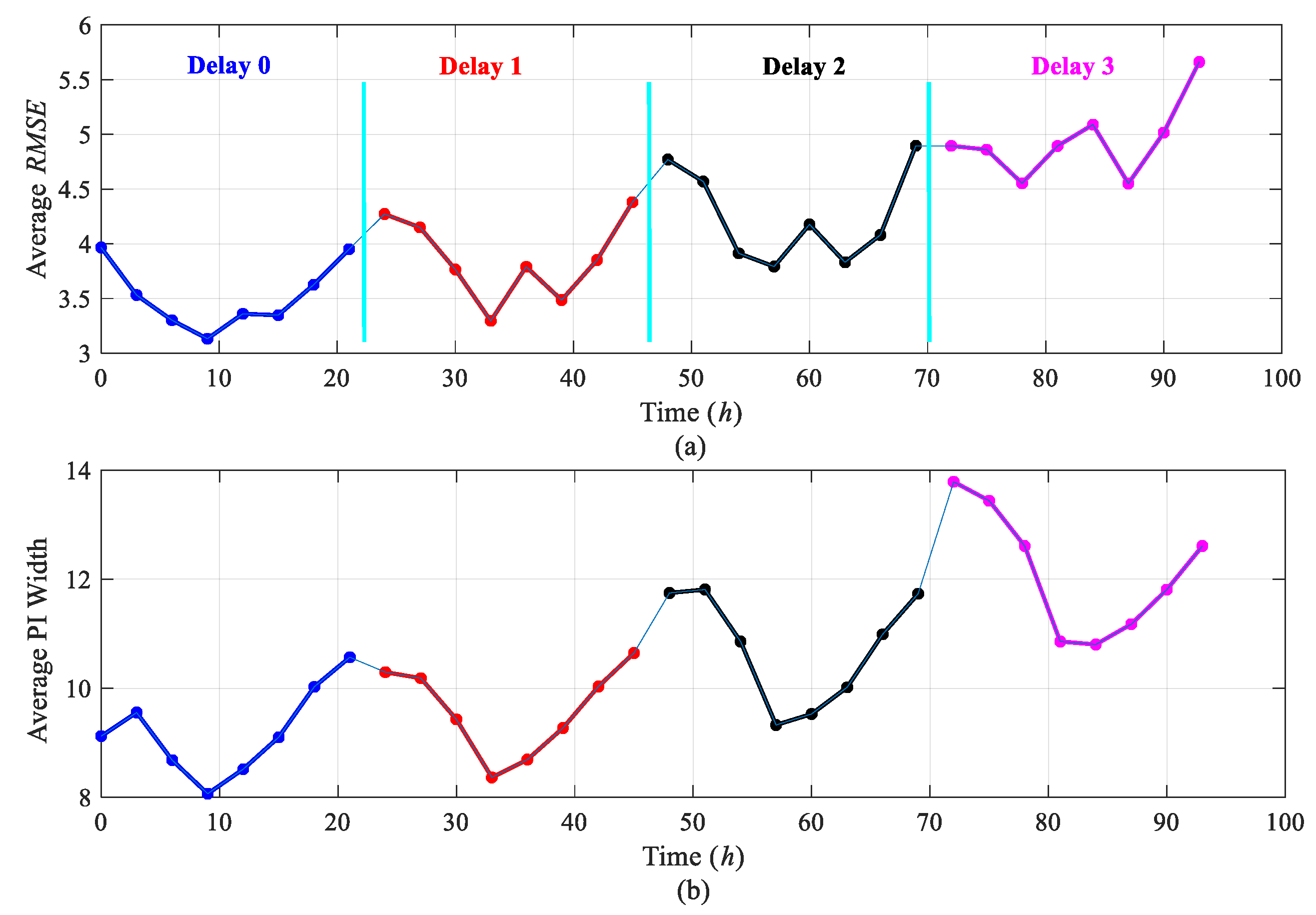
The ensemble approach of Section 2 trained on the 2011–2012 data is used for the predictions of the energy productions of the 2013 test data for a time horizon (hereafter called delays) of four days, Δ t = 93 h; namely, delays 1–4 correspond to the predictions in the time intervals [ 0 21 ] ,   [ 24 45 ] ,   [ 48 69 ] and [ 72 93 ] , respectively. Figure 10a shows the average Root Mean Square Error (RMSE) used for evaluating the accuracy of the production predictions on the overall test data, whereas Figure 10b shows the average widths of the corresponding PIs at each prediction hour. One can easily recognize that the larger the time horizon of the prediction, the larger the ensemble prediction error, and, coherently, the larger the PI’s width.
For clarification purposes, Figure 11 shows an example of the energy production predictions of 4 days ahead (i.e., Δ t = 93 h) with the corresponding BS PIs estimates. One can easily recognize that, for large production values, the PIs are enlarged to accommodate the large uncertainty that affects the predictions. In contrast, for small production values, the PIs are shortened due to the small uncertainty that affects the predictions.
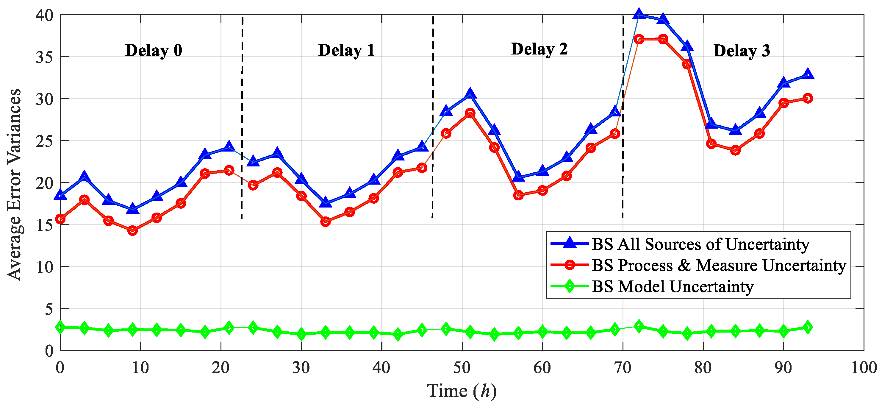
As the last remark, the decomposition of the sources of uncertainty that affect the energy production predictions has shown that (Figure 12):
  • As expected, process and measure errors (circle) are increasing with the time horizon of the prediction due to the weather forecast errors;
  • Process and measure errors are following the variability of the electricity production. This explains the variability in the widths of the obtained PIs;
  • Model error (diamond) is stable with respect to the time horizon of the prediction;
  • The overall error (triangle) is consequently increasing with the time horizon of the prediction and following the variability of the electricity productions.

6. Conclusions

In this work, we have considered the problem of quantifying the uncertainty that affects the predictions of the energy productions of a wind plant. The uncertainty quantification is carried out by constructing Prediction Intervals (PIs) with a predefined confidence level (e.g., 0.8). To this aim, the Bootstrap (BS) technique has been applied, and its capabilities have been verified on a real case study of a wind plant located in Italy. The obtained PIs have been evaluated by considering two indicators: (1) the coverage, i.e., the fraction of the true/actual energy productions which actually fall within the PIs, and (2) the PI width. Results show that the BS technique is superior and more informative for the electric grid operators than a technique based on the use of the quantiles of the ensemble model predictions, which is currently used by the plant owner, and the Mean-Variance Estimation (MVE). In practice, only the proposed method is able to cover within the prediction intervals a fraction of the true production values larger than the predefined confidence interval, which confirms its capability of properly describing all uncertainty sources. The PIs obtained by the BS technique have been further analyzed in terms of the different weather conditions experienced by the wind plant and the time horizon of the predictions. Future work will be devoted to (1) optimizing the PIs in order to obtain a trade-off between PI coverage and PI width, which is satisfactory for the decision-maker; (2) developing a framework for the effective use of the PIs in the formulation of energy bidding strategies.

Author Contributions

S.A.-D., P.B. and E.Z. were responsible for the conceptualization, methodology, software, validation, formal analysis, investigation, data curation, writing—original draft, writing—review and editing, visualization, supervision, and project administration, and M.L. was responsible for the resources, validation, project administration, and writing—review and editing. All authors have read and agreed to the published version of the manuscript.

Funding

This research received no external funding.

Institutional Review Board Statement

Not applicable.

Informed Consent Statement

Not applicable.

Data Availability Statement

Data was obtained from Edison Spa. Data sharing is not applicable to this article for confidentiality reasons.

Acknowledgments

The participation of Enrico Zio to this research is partially supported by the China NSFC under grant number 71231001.

Conflicts of Interest

The authors declare no conflict of interest.

Abbreviations

The following acronyms/notations are used in this manuscript:
Acronyms
ANNsArtificial Neural Networks
SVMsSupport Vector Machines
k-nnk-nearest neighbors
SVRSupport Vector Regression
GPRGaussian Process Regression
BTBoosted Trees
RFRandom Forest
GRFGeneralized Random Forest
BSBootstrap
LUBELower Upper Bound Estimation
MVEMean-Variance Estimation
PSOParticle Swarm Optimization
PCAPrincipal Component Analysis
FCMFuzzy C-Means
DBDavies-Bouldin
RMSERoot Mean Square Error
BAGGINGBootstrapping AGGregatING
SASimple Average
SMSimple Median
GWAGlobally Weighted Average
LWALocally Weighted Average
LFLocal Fusion
Notation
X a l l Overall available dataset
WF Weather-forecasting data
P Energy productions
WF a l l Overall available weather-forecasting data
P a l l Overall available energy productions
X t r a i n Training dataset
N t r a i n Number of available training patterns
WF t r a i n Weather-forecasting data used for training
P t r a i n Energy productions used for training
X B S t r a i n Training dataset used in BS
X M V E t r a i n Training dataset used in MVE
X v a l i d Validation dataset
N v a l i d Number of available validation patterns
X t e s t Test dataset
N t e s t Number of available test patterns
WF v a l i d Weather-forecasting data used for validation
P v a l i d Actual energy productions of the validation dataset
P ^ v a l i d Energy production predictions of the validation dataset
t j A generic j -th test pattern
W F j t e s t Weather-forecasting data used for testing at time t j
h Index of base model, h = 1 , , H
H Number of base models in the ensemble
P j Actual energy production at time t j
P ^ j h Predicted energy production obtained by the h -th base model at time t j
P ^ j e n s e m b l e Predicted energy production obtained by the ensemble at time t j
P ^ h Predicted energy production obtained by the h -th base model
P ^ e n s e m b l e Predicted energy production obtained by the ensemble
w h Weight of the h -th base model
αPredefined confidence level
P I Prediction Interval
P I α PI of confidence level α
P ^ j l o w e r Lower production prediction obtained at time t j
P ^ j u p p e r Upper production prediction obtained at time t j
ε Prediction error
σ ε 2 Overall prediction error variance
σ W F 2 Variance caused by weather-forecast errors
σ P R 2 Variance caused by the stochastic variability of the physical process
σ M O 2 Variance caused by the ensemble model error
σ M O 2 v a l i d Variance caused by the ensemble model error on the validation dataset
σ ε 2 j t e s t Overall prediction error variance obtained for the j -th test pattern
σ W F 2 j t e s t Variance caused by weather-forecast errors obtained for the j -th test pattern
σ P R 2 j t e s t Variance caused by the stochastic variability of the physical process obtained for the j-th test pattern
σ M O 2 j t e s t Variance caused by the ensemble model error obtained for the j -th test pattern
P ^ j t e s t Predicted energy production obtained by the ensemble for the j -th test pattern
C d o f α ( 1 α ) / 2 quantile of a Student t-distribution with a number of degrees of freedom
Δ t Prediction horizon
F Number of weather features available
F * Optimum number of weather features obtained by the PCA
u, vHorizontal and vertical wind speed components
S Possible number of the weather conditions (groups) experienced by the wind plant
C o p t Optimum number of weather conditions groups

Appendix A. The MVE Estimation Technique for PIs Estimation

The flowchart of the Mean-Variance Estimation (MVE) technique for the estimation of the unknown σ ε 2 , and the associated PIs, is sketched in Figure 1. There are two steps [55]:
Step 1: Building the MVE training dataset. Let us assume that we have available a dataset of weather-forecasting data and their associated energy productions, X a l l = [ W F a l l , P a l l ] . This dataset is portioned into two datasets: a training dataset X t r a i n = [ W F t r a i n , P t r a i n ] for building the ensemble of ANN models and a validation dataset X v a l i d = [ W F v a l i d , P v a l i d ] for providing estimates of the energy productions, P ^ v a l i d , whose true productions P v a l i d are already known. The MVE training dataset X M V E t r a i n = [ W F v a l i d , ( P v a l i d P ^ v a l i d ) 2 ] can then be prepared with the weather-forecasting data of the validation dataset, W F v a l i d , and the squared prediction errors, ( P v a l i d P ^ v a l i d ) 2 , on the validation dataset.
Step 2: Constructing the MVE PIs of the test pattern. With the MVE training dataset, a dedicated feedforward ANN is developed for providing, at time t j , an estimate of the variance, σ ε 2 j t e s t , associated with a general test pattern of weather-forecasting data, W F j t e s t . To ensure a strictly positive variance estimate, an exponential activation function is used.
Thus, a dedicated feedforward ANN characterized by an architecture of three layers (input, hidden, and output) and seven hidden neurons are developed to estimate the prediction error variance with the MVE technique.
Finally, the PI with a confidence level equal to α % of the test pattern at the time t j is obtained as per Equation (A1) [55,57]:
[ P ^ j l o w e r , P ^ j u p p e r ] = P ^ j t e s t ± C d o f α . σ ε 2 j t e s t
where P ^ j t e s t is the energy production predicted by the ANN ensemble for the test pattern at a time t j and C d o f α is the ( 1 α ) / 2 quantile of Student t-distribution with a number of degrees of freedom equal to the number of ensemble models H .

References

  1. International Energy Agency (IAEA). Global Energy Review 2021; International Energy Agency (IAEA): Paris, France, 2021. [Google Scholar]
  2. Global Wind Energy Council (GWEC). Global Wind Report 2021; Global Wind Energy Council (GWEC): Brussels, Belgium, 2021. [Google Scholar]
  3. International Renewable Energy Agency (IRENA). Renewable Capacity Statistics 2021; International Renewable Energy Agency: Abu Dhabi, United Arab Emirates, 2021. [Google Scholar]
  4. WindEurope. Wind Energy in Europe-2020 Statistics and the Outlook for 2021–2025; WindEurope: Brussels, Belgium, 2020. [Google Scholar]
  5. Kosmadakis, G.; Karellas, S.; Kakaras, E. Renewable and Conventional Electricity Generation Systems: Technologies and Diversity of Energy Systems. In Renewable Energy Governance: Complexities and Challenges; Michalena, E., Hills, J.M., Eds.; Springer: London, UK, 2013; pp. 9–30. ISBN 978-1-4471-5595-9. [Google Scholar]
  6. Sideratos, G.; Hatziargyriou, N.D. An advanced statistical method for wind power forecasting. IEEE Trans. Power Syst. 2007, 22, 258–265. [Google Scholar] [CrossRef]
  7. Foley, A.M.; Leahy, P.G.; Marvuglia, A.; McKeogh, E.J. Current methods and advances in forecasting of wind power generation. Renew. Energy 2012, 37, 1–8. [Google Scholar] [CrossRef] [Green Version]
  8. Najeebullah; Zameer, A.; Khan, A.; Javed, S.G. Machine Learning based short term wind power prediction using a hybrid learning model. Comput. Electr. Eng. 2015, 45, 122–133. [Google Scholar] [CrossRef]
  9. Bessa, R.J.; Miranda, V.; Gama, J. Entropy and correntropy against minimum square error in offline and online three-day ahead wind power forecasting. IEEE Trans. Power Syst. 2009, 24, 1657–1666. [Google Scholar] [CrossRef]
  10. Qin, G.; Yan, Q.; Zhu, J.; Xu, C.; Kammen, D.M. Day-ahead wind power forecasting based on wind load data using hybrid optimization algorithm. Sustainability 2021, 13, 1164. [Google Scholar] [CrossRef]
  11. Zhen, H.; Niu, D.; Yu, M.; Wang, K.; Liang, Y.; Xu, X. A hybrid deep learning model and comparison for wind power forecasting considering temporal-spatial feature extraction. Sustainability 2020, 12, 9490. [Google Scholar] [CrossRef]
  12. Soman, S.S.; Zareipour, H.; Malik, O.; Mandal, P. A review of wind power and wind speed forecasting methods with different time horizons. In Proceedings of the North American Power Symposium 2010, Arlington, TX, USA, 26–28 September 2010; pp. 1–8. [Google Scholar]
  13. Ernst, B.; Reyer, F.; Vanzetta, J. Wind power and photovoltaic prediction tools for balancing and grid operation. In Proceedings of the 2009 CIGRE/IEEE PES Joint Symposium Integration of Wide-Scale Renewable Resources Into the Power Delivery System, Calgary, AB, Canada, 29–31 July 2009; pp. 1–9. [Google Scholar]
  14. Costa, A.; Crespo, A.; Navarro, J.; Lizcano, G.; Madsen, H.; Feitosa, E. A review on the young history of the wind power short-term prediction. Renew. Sustain. Energy Rev. 2008, 12, 1725–1744. [Google Scholar] [CrossRef] [Green Version]
  15. Ernst, B.; Oakleaf, B.; Ahlstrom, M.L.; Lange, M.; Moehrlen, C.; Lange, B.; Focken, U.; Rohrig, K. Predicting the wind. IEEE Power Energy Mag. 2007, 5, 78–89. [Google Scholar] [CrossRef]
  16. Lange, M.; Focken, U. Physical Approach to Short-Term Wind Power Prediction; Springer: Berlin, Germany, 2006. [Google Scholar]
  17. Li, C.; Lin, S.; Xu, F.; Liu, D.; Liu, J. Short-term wind power prediction based on data mining technology and improved support vector machine method: A case study in Northwest China. J. Clean. Prod. 2018, 205, 909–922. [Google Scholar] [CrossRef]
  18. Thordarson, F.Ö.; Madsen, H.; Nielsen, H.A.; Pinson, P. Conditional weighted combination of wind power forecasts. Wind Energy 2010, 13, 751–763. [Google Scholar] [CrossRef]
  19. Tascikaraoglu, A.; Uzunoglu, M. A review of combined approaches for prediction of short-term wind speed and power. Renew. Sustain. Energy Rev. 2014, 34, 243–254. [Google Scholar] [CrossRef]
  20. Rahman, M.M.; Shakeri, M.; Tiong, S.K.; Khatun, F.; Amin, N.; Pasupuleti, J.; Hasan, M.K. Prospective methodologies in hybrid renewable energy systems for energy prediction using artificial neural networks. Sustainability 2021, 13, 2393. [Google Scholar] [CrossRef]
  21. Ioakimidis, C.S.; Genikomsakis, K.N.; Dallas, P.I.; Lopez, S. Short-term wind speed forecasting model based on ANN with statistical feature parameters. In Proceedings of the IECON 2015-41st Annual Conference of the IEEE Industrial Electronics Society, Yokohama, Japan, 9–12 November 2015; pp. 000971–000976. [Google Scholar]
  22. Ramasamy, P.; Chandel, S.S.; Yadav, A.K. Wind speed prediction in the mountainous region of India using an artificial neural network model. Renew. Energy 2015, 80, 338–347. [Google Scholar] [CrossRef]
  23. Sharifzadeh, M.; Sikinioti-Lock, A.; Shah, N. Machine-learning methods for integrated renewable power generation: A comparative study of artificial neural networks, support vector regression, and Gaussian Process Regression. Renew. Sustain. Energy Rev. 2019, 108, 513–538. [Google Scholar] [CrossRef]
  24. Jursa, R.; Rohrig, K. Short-term wind power forecasting using evolutionary algorithms for the automated specification of artificial intelligence models. Int. J. Forecast. 2008, 24, 694–709. [Google Scholar] [CrossRef]
  25. Di Piazza, A.; Di Piazza, M.C.; La Tona, G.; Luna, M. An artificial neural network-based forecasting model of energy-related time series for electrical grid management. Math. Comput. Simul. 2021, 184, 294–305. [Google Scholar] [CrossRef]
  26. Wang, J.; Sun, J.; Zhang, H. Short-term wind power forecasting based on support vector machine. In Proceedings of the 2013 5th International Conference on Power Electronics Systems and Applications(PESA), Hong Kong, China, 11–13 December 2013; pp. 1–5. [Google Scholar]
  27. Kramer, O.; Gieseke, F. Short-Term Wind Energy Forecasting Using Support Vector Regression. In Soft Computing Models in Industrial and Environmental Applications, 6th International Conference SOCO 2011; Corchado, E., Snášel, V., Sedano, J., Hassanien, A.E., Calvo, J.L., Ślȩzak, D., Eds.; Springer: Berlin/Heidelberg, Germany, 2011; pp. 271–280. ISBN 978-3-642-19644-7. [Google Scholar]
  28. Kramer, N.A.; Treiber, O. Evolutionary feature weighting for wind power prediction with nearest neighbor regression. In Proceedings of the 2015 IEEE Congress on Evolutionary Computation (CEC), Sendai, Japan, 25–28 May 2015; pp. 332–337. [Google Scholar]
  29. Yesilbudak, M.; Sagiroglu, S.; Colak, I. A novel implementation of kNN classifier based on multi-tupled meteorological input data for wind power prediction. Energy Convers. Manag. 2017, 135, 434–444. [Google Scholar] [CrossRef]
  30. Chen, N.; Qian, Z.; Nabney, I.T.; Meng, X. Wind power forecasts using gaussian processes and numerical weather prediction. IEEE Trans. Power Syst. 2014, 29, 656–665. [Google Scholar] [CrossRef] [Green Version]
  31. Mellit, A.; Kalogirou, S.A. Artificial intelligence techniques for photovoltaic applications: A review. Prog. Energy Combust. Sci. 2008, 34, 574–632. [Google Scholar] [CrossRef]
  32. Luchetta, A.; Manetti, S.; Piccirilli, M.C.; Reatti, A.; Corti, F.; Catelani, M.; Ciani, L.; Kazimierczuk, M.K. MLMVNNN for Parameter Fault Detection in PWM DC-DC Converters and Its Applications for Buck and Boost DC-DC Converters. IEEE Trans. Instrum. Meas. 2019, 68, 439–449. [Google Scholar] [CrossRef]
  33. De Leon-Aldaco, S.E.; Calleja, H.; Aguayo Alquicira, J. Metaheuristic Optimization Methods Applied to Power Converters: A Review. IEEE Trans. Power Electron. 2015, 30, 6791–6803. [Google Scholar] [CrossRef]
  34. Han, S.; Liu, Y.; Yan, J. Neural network ensemble method study for wind power prediction. In Proceedings of the 2011 AsiaPacific Power and Energy Engineering Conference APPEEC 2011, Wuhan, China, 25–28 March 2011. [Google Scholar]
  35. Bonissone, P.P.; Xue, F.; Subbu, R. Fast meta-models for local fusion of multiple predictive models. Appl. Soft Comput. J. 2011, 11, 1529–1539. [Google Scholar] [CrossRef]
  36. Lee, J.; Wang, W.; Harrou, F.; Sun, Y. Wind Power Prediction Using Ensemble Learning-Based Models. IEEE Access 2020, 8, 61517–61527. [Google Scholar] [CrossRef]
  37. Zameer, A.; Arshad, J.; Khan, A.; Raja, M.A.Z. Intelligent and robust prediction of short term wind power using genetic programming based ensemble of neural networks. Energy Convers. Manag. 2017, 134, 361–372. [Google Scholar] [CrossRef]
  38. Al-Dahidi, S.; Baraldi, P.; Zio, E.; Legnani, E. A Dynamic Weighting Ensemble Approach for Wind Energy Production Prediction. In Proceedings of the 2017 2nd International Conference on System Reliability and Safety, Milan, Italy, 20–22 December 2017; pp. 296–302. [Google Scholar]
  39. Khosravi, A.; Nahavandi, S.; Creighton, D.; Naghavizadeh, R. Uncertainty quantification for wind farm power generation. In Proceedings of the 2012 International Joint Conference on Neural Networks (IJCNN), Brisbane, Australia, 10–15 June 2012; pp. 1–6. [Google Scholar]
  40. Holttinen, H.; Miettinen, J.; Sillanpää, S. Wind Power Forecasting Accuracy and Uncertainty in Finland; VTT Technical Research Centre of Finland: Espoo, Finland, 2013; ISBN 9789513879853. [Google Scholar]
  41. Khosravi, A.; Nahavandi, S.; Creighton, D.; Atiya, A.F. A comprehensive review of neural network-based prediction intervals and new advances. IEEE Trans. Neural Netw. 2011, 22, 1341–1356. [Google Scholar] [CrossRef]
  42. Dupré, A.; Drobinski, P.; Badosa, J.; Briard, C.; Tankov, P. The economic value of wind energy nowcasting. Energies 2020, 13, 5266. [Google Scholar] [CrossRef]
  43. Li, Z.; Zhang, Z. Day-Ahead and Intra-Day Optimal Scheduling of Integrated Energy System Considering Uncertainty of Source & Load Power Forecasting. Energies 2021, 14, 2539. [Google Scholar]
  44. Korprasertsak, N.; Leephakpreeda, T. Robust short-term prediction of wind power generation under uncertainty via statistical interpretation of multiple forecasting models. Energy 2019, 180, 387–397. [Google Scholar] [CrossRef]
  45. Hwang, J.G.; Ding, A.A. Prediction Intervals for Artificial Neural Networks. J. Am. Stat. Assoc. 1997, 92, 748–757. [Google Scholar] [CrossRef]
  46. Ho, S.L.; Xie, M.; Tang, L.C.; Xu, K.; Goh, T.N. Neural network modeling with confidence bounds: A case study on the solder paste deposition process. IEEE Trans. Electron. Packag. Manuf. 2001, 24, 323–332. [Google Scholar] [CrossRef]
  47. Heskes, T. Practical confidence and prediction intervals. In Advances in Neural Information Processing Systems 9, Proceedings of the 9th International Conference on Neural Information Processing Systems, Denver, CO, USA, 2–5 December 1996; MIT Press: Cambridge, MA, USA, 1997; pp. 176–182. [Google Scholar]
  48. Ak, R.; Vitelli, V.; Zio, E. Uncertainty modeling in wind power generation prediction by neural networks and bootstrapping. In Proceedings of the Safety, Reliability and Risk Analysis: Beyond the Horizon-Proceedings of the European Safety and Reliability Conference, ESREL 2013, Amsterdam, The Netherlands, 29 September–3 October 2013. [Google Scholar]
  49. Errouissi, R.; Cardenas-Barrera, J.; Meng, J.; Castillo-Guerra, E.; Gong, X.; Chang, L. Bootstrap prediction interval estimation for wind speed forecasting. In Proceedings of the 2015 IEEE Energy Conversion Congress and Exposition (ECCE 2015), Montreal, QC, Canada, 20–24 September 2015; pp. 1919–1924. [Google Scholar]
  50. Chan, W.S.; Cheung, S.H.; Wu, K.H. Multiple forecasts with autoregressive time series models: Case studies. Math. Comput. Simul. 2004, 64, 421–430. [Google Scholar] [CrossRef]
  51. Khosravi, A.; Nahavandi, S.; Creighton, D.; Atiya, A.F. Lower upper bound estimation method for construction of neural network-based prediction intervals. IEEE Trans. Neural Netw. 2011, 22, 337–346. [Google Scholar] [CrossRef]
  52. Wen, P.; Zhang, S.; Xing, Y.; Huo, L.; Bohlooli, N. A novel method based on lower–upper bound approximation to predict the wind energy. J. Clean. Prod. 2020, 259, 120458. [Google Scholar] [CrossRef]
  53. Liu, F.; Li, C.; Xu, Y.; Tang, G.; Xie, Y. A new lower and upper bound estimation model using gradient descend training method for wind speed interval prediction. Wind Energy 2020, 24, 290–304. [Google Scholar] [CrossRef]
  54. Quan, H.; Srinivasan, D.; Khosravi, A. Short-term load and wind power forecasting using neural network-based prediction intervals. IEEE Trans. Neural Netw. Learn. Syst. 2014, 25, 303–315. [Google Scholar] [CrossRef] [PubMed]
  55. Nix, D.A.; Weigend, A.S. Estimating the mean and variance of the target probability distribution. In Proceedings of the 1994 IEEE International Conference on Neural Networks, Orlando, FL, USA, 28 June–2 July 1994; Volume 1, pp. 55–60. [Google Scholar]
  56. Khosravi, A.; Nahavandi, S. An optimized mean variance estimation method for uncertainty quantification of wind power forecasts. Int. J. Electr. Power Energy Syst. 2014, 61, 446–454. [Google Scholar] [CrossRef]
  57. Baraldi, P.; Mangili, F.; Zio, E. Ensemble of bootstrapped models for the prediction of the remaining useful life of a creeping turbine blade. In Proceedings of the 2012 IEEE Conference on Prognostics and Health Management (PHM), Denver, CO, USA, 18–21 June 2012; pp. 1–8. [Google Scholar]
  58. Al-Dahidi, S.; Ayadi, O.; Alrbai, M.; Adeeb, J. Ensemble Approach of Optimized Artificial Neural Networks for Solar Photovoltaic Power Prediction. IEEE Access 2019, 7, 81741–81758. [Google Scholar] [CrossRef]
  59. Jaulin, L. Applied Interval Analysis: With Examples in Parameter and State Estimation; Robust Control and Robotics; Springer: Berlin/Heidelberg, Germany, 2001. [Google Scholar]
  60. Jolliffe, I.T. Principal Component Analysis. J. Am. Stat. Assoc. 2002, 98, 487. [Google Scholar]
  61. Schölkopf, B.; Smola, A.; Müller, K.R. Kernel Principal Component Analysis. Comput. Vis. Math. Methods Med. Biomed. Image Anal. 2012, 1327, 583–588. [Google Scholar]
  62. Bezdek, J.C. Pattern Recognition with Fuzzy Objective Function Algorithms; Springer: Boston, MA, USA, 1981; ISBN 0-306-40671-3. [Google Scholar]
  63. Baraldi, P.; Di Maio, F.; Rigamonti, M.; Zio, E.; Seraoui, R. Unsupervised clustering of vibration signals for identifying anomalous conditions in a nuclear turbine. J. Intell. Fuzzy Syst. 2013, 28, 1723–1731. [Google Scholar] [CrossRef]
  64. Davies, D.L.; Bouldin, D.W. A cluster separation measure. IEEE Trans. Pattern Anal. Mach. Intell. 1979, 1, 224–227. [Google Scholar] [CrossRef] [PubMed]
  65. Al-Dahidi, S.; Di Maio, F.; Baraldi, P.; Zio, E. A locally adaptive ensemble approach for data-driven prognostics of heterogeneous fleets. Proc. Inst. Mech. Eng. Part O J. Risk Reliab. 2017, 231, 350–363. [Google Scholar] [CrossRef] [Green Version]
  66. Maqsood, I.; Khan, M.; Abraham, A. An ensemble of neural networks for weather forecasting. Neural Comput. Appl. 2004, 13, 112–122. [Google Scholar] [CrossRef]
  67. Brown, G.; Wyatt, J.; Harris, R.; Yao, X. Diversity creation methods: A survey and categorisation. Inf. Fusion 2005, 6, 5–20. [Google Scholar] [CrossRef]
  68. Baraldi, P.; Mangili, F.; Zio, E. A Kalman filter-based ensemble approach with application to turbine creep prognostics. IEEE Trans. Reliab. 2012, 61, 966–977. [Google Scholar] [CrossRef]
  69. Polikar, R. Ensemble based systems in decision making. Circuits Syst. Mag. IEEE 2006, 6, 21–45. [Google Scholar] [CrossRef]
  70. Breiman, L. Bagging Predictors. Mach. Learn. 1996, 24, 123–140. [Google Scholar] [CrossRef] [Green Version]
  71. Schapire, R.E. The Strength of Weak Learnability. Mach. Learn. 1990, 5, 197–227. [Google Scholar] [CrossRef] [Green Version]
  72. Freund, Y.; Schapire, R.E. A Decision-Theoretic Generalization of On-Line Learning and an Application to Boosting. J. Comput. Syst. Sci. 1997, 55, 119–139. [Google Scholar] [CrossRef] [Green Version]
  73. Efron, B.; Tibshirani, R.J. An Introduction to the Bootstrap. Refrig. Air Cond. 1993, 57, 436. [Google Scholar]
  74. Bishop, C.M. Neural networks for pattern recognition. J. Am. Stat. Assoc. 1995, 92, 482. [Google Scholar]
  75. Liu, Y.; Yao, X.; Higuchi, T. Evolutionary ensembles with negative correlation learning. IEEE Trans. Evol. Comput. 2000, 4, 380–387. [Google Scholar]
  76. Hadjicharalambous, M.; Polycarpou, M.M.; Panayiotou, C.G. Neural network-based construction of online prediction intervals. Neural Comput. Appl. 2020, 32, 6715–6733. [Google Scholar] [CrossRef]
  77. Onanena, R.; Oukhellou, L.; Come, E.; Jemei, S. Fuel Cell Health Monitoring Using Self Organizing Maps. Chem. Eng. Trans. 2013, 33, 1021–1026. [Google Scholar]
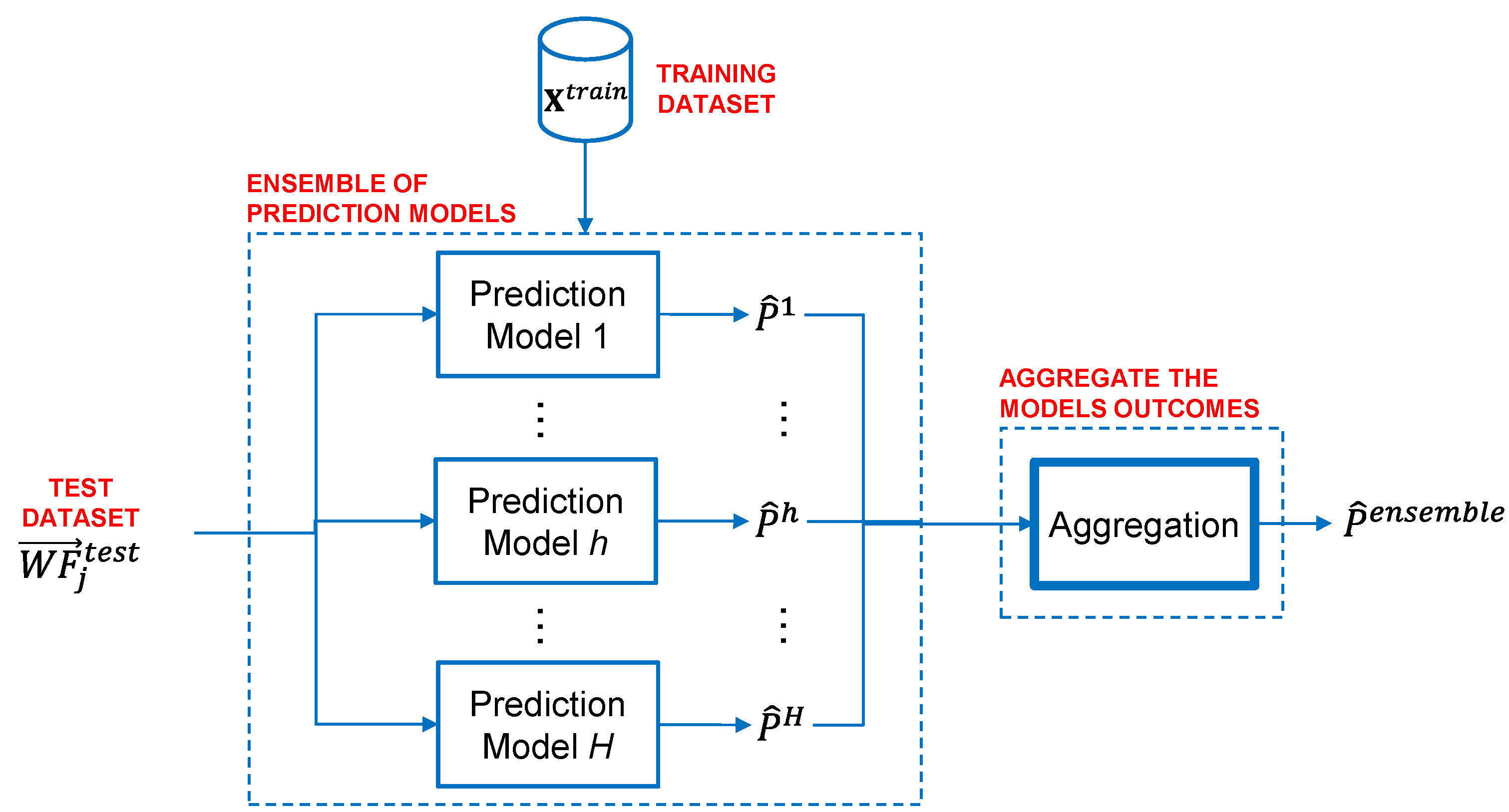
Figure 1. Scheme of the ensemble of models used for energy production prediction.
Sustainability 13 06417 g001
Figure 2. Scheme of the application of the BS technique to the estimation of PIs of energy production predictions.
Sustainability 13 06417 g002
Figure 3. (a) Wind speed; (b) related wind energy productions of the year 2013.
Sustainability 13 06417 g003
Figure 4. Energy production predictions (squares) provided by the ensemble of ANNs and the corresponding true values (circles) for two different days of the year 2013.
Sustainability 13 06417 g004
Figure 5. Comparison of the PIs provided by the BS (shaded area), Quantile (triangles), and MVE (diamonds) techniques for two different days of the year 2013.
Sustainability 13 06417 g005
Figure 6. (a) Variance accounted by each principal component; (b) overall dataset in the space of the two identified principal components.
Sustainability 13 06417 g006
Figure 7. (a) Reconstruction of a wind speed signal using the identified principal components; (b) corresponding residuals of the reconstructions.
Sustainability 13 06417 g007
Figure 8. (a) DB values vs. number of groups; (b) the obtained groups in the space of the identified principal components.
Sustainability 13 06417 g008
Figure 9. (a) Average PI widths; (b) average PI coverage values with respect to the three weather forecast groups; (c) examples of the estimated PIs of few data in the three weather conditions.
Sustainability 13 06417 g009
Figure 10. (a) Average RMSE and (b) average PI width obtained by the BS technique for four-day ahead predictions.
Sustainability 13 06417 g010
Figure 11. An example of the estimated PIs obtained by the BS technique for four day ahead predictions.
Sustainability 13 06417 g011
Figure 12. Average decomposition of the three sources of uncertainty and the total error of the four-day ahead predictions.
Sustainability 13 06417 g012
Table 1. Comparison of the PIs estimated by BS, the Quantile technique adopted by the plant owner, and the MVE technique.
Mean PI WidthPI Coverage Probability
Quantile4.6250.3352
MVE11.670.6534
BS12.20.81
Publisher’s Note: MDPI stays neutral with regard to jurisdictional claims in published maps and institutional affiliations.