Abstract
Establishing a functional financial sector has been one of the pillars of transition to a functional market economy over the last three decades in the CEE region. The present paper provides a comprehensive analysis of the relationship between credit and economic growth in selected CEE countries, namely, Czechia, Romania, Poland and Hungary, aiming to answer questions related to (i) the role of the banking sector in fostering sustainable economic growth and the causality direction between the financial and real sector, (ii) the relationship between consumption and investment and certain categories of loans and (iii) the identification of loan supply shocks and their role in explaining the dynamics associated with other macroeconomic variables. Using a time-varying parameter structural vector autoregression model with stochastic volatility (TVP-SVAR) and sign restrictions, we identify a non-financial corporations (NFC) credit supply shock and an investment shock. Potential policy solutions to ensure a sound contribution of the financial sector to economic growth in the analyzed economies relate to the strong relationship identified between the two variables. From this perspective, the study is among the first to employ a robust dynamic framework for assessing the role of the financial sector in fostering sustainable economic growth in European emerging market economies.
1. Introduction
Over the last decades and in the context of globalization, the relationship between economic development and financial intermediation has become increasingly tighter. However, during episodes of turmoil such as the Global Financial Crisis, the financial sector can potentially become a source of systemic risk amplification through contagion effects or through a severe contraction in the supply of credit and, as a result, significantly affect the real economy.
Analyzing the relationship between the financial sector and the real economy in Central and Eastern Europe warrants a thorough understanding of the significant structural changes the studied economies have experienced over the last three decades. In this regard, this paper focuses on the cases of Czechia, Romania, Hungary and Poland. In all four countries, the transition from a planned to an open market economy in the beginning of the 1990s prompted a wide economic reform in which the development of the financial sector served as one of the key elements for a successful transition. Other important milestones were the capital account liberalization process, the EU accession which triggered high capital inflows in the run up to the Global Financial Crisis, the period of economic rebalancing following the crisis and the renewed economic growth period accompanied by an upturn in the financial cycle.
Transforming the financial sector from a profit- to a sustainability-oriented driver of economic growth will be the main challenge over the medium term for the countries included in the analysis. Aligning the financing priorities with the structural changes required to successfully transition to sustainable growth models will require coordinated efforts to adapt business models, strategies to promote financial inclusion, investment in green projects and financing transitions to less carbon intensive activities.
As detailed in Section 2, the literature review, analyses on the relationship between credit and economic growth in the CEE region are scarce, mainly due to the lack of statistical data. In this context, the present paper aims to bring a new perspective by providing a comprehensive analysis of Poland, Czechia, Romania and Hungary, after 30 years of financial sector development. Towards these objectives, we believe our study addresses this research gap identified in the literature, through a robust modeling framework and multiple approaches to assess the complex relationship between the financial sector and the real economy.
Therefore, the study aims at finding answers to questions related to (i) the role of the banking sector in fostering sustainable economic growth and the causality direction between the financial and real sector, (ii) the relationship between consumption and investment and certain types of loans and (iii) the identification of loan supply shocks and their role in explaining dynamics associated with other macroeconomic variables included in a structural model.
The analysis is paramount to assess the current role of the financial sector in these economies, required to trace out the structural changes needed to ensure a future sustainable development. Objectives such as (i) expanding financial inclusion, (ii) fostering green finance, (iii) maximizing societal welfare instead of profits should be pursued by policy makers as well as market participants in order to reposition the financial sector on a sustainable path while ensuring a positive contribution to the real economy.
In terms of methodology, Section 3 starts by describing a naive approach for assessing the relationship between economic growth and credit: estimating time-varying linear regressions between economic activity and the supply of credit from the financial sector. The analyzed dataset spans from 2004 to 2019, capturing the early stages of development of the banking sector in the EU accession context. The paper continues with a TVP–VAR model with stochastic volatility and sign restrictions designed to identify the role played by NFC credit supply shocks over the main macroeconomic variables in each of the analyzed CEE members. Section 4 discusses the main results of the implemented models and Section 5 presents the concluding remarks.
2. Literature Review
As highlighted by the data extracted from the World Bank database for over 150 countries or regions from all around the world, when comparing 1995 data with 2015 data, the statistical significance of the correlation between economic development and financial intermediation surges while the slope coefficient almost doubles in absolute size (Figure 1).
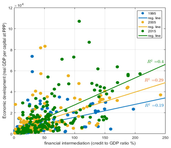
Figure 1.
The relationship between economic development and financial intermediation. Note: economic development is measured as real GDP per capita in USD at PPP while financial intermediation is defined as private sector credit to GDP ratio. Source: World Bank Database.
In this context, the relationship between the credit and the real economy was widely investigated over time and has gained increasing importance in the context of a globalization process conducted in the post-crisis period. Moreover, as highlighted by Claessens et al. [1], most of the economic literature indicate that credit markets have a dual role in macroeconomics, being both a propagation mechanism of shocks originated in other markets and a source of shocks driving business cycle fluctuations, in particular credit supply shocks, that can have an important contribution to the macroeconomic variables’ evolution.
The main approaches on this matter have been defined by two schools of thought with completely different perspectives. Firstly, renowned economists such as Schumpeter [2], Goldsmith [3], McKinnon [4] and Shaw [5] supported the idea that financial intermediation plays an important role for the long-run economic growth. On the other hand, Robinson [6] believed that robust economic growth perspectives lead to the development of a sound financial sector. Another theory that sharply contradicts Schumpeter’s assumptions was founded by Lucas [7], stating that economists “badly over-stress” the role financial factors play in economic growth.
Păun et al. [8] found that the sophistication of financial system and financial inclusion positively influences economic growth and development. Other earlier studies, such as Petkovsky and Kyojevsky [9], found that, in the case of 16 transition countries from Central and Eastern Europe, from 1991 to 2011, the contribution of the relatively underdeveloped credit markets to growth has been limited. Loayza et al. [10] concluded that financial deepening leads to a trade-off between higher economic growth and higher crisis risk-for middle-income countries; the positive growth effects can outweigh the negative crisis impact.
In terms of sign restriction applied to identify credit supply shocks, the empirical literature references worth highlighting are the methodologies proposed by Faust [11], Canova and De Nicolo [12], and Uhlig [13]. Furthermore, Bean et al. [14] and De Nicolo and Lucchetta [15] proposed that credit supply shocks can be isolated from demand shocks by restricting supply shocks to affect credit volume and loan rates in different directions. However, Meeks [16] criticizes previous literature and argues that restrictions must be imposed only on pure financial variables. Hristov et al. [17] also contradict previous studies and propose that the response of monetary policy should go in the opposite direction of the response of the lending rate when credit supply shocks hit the economy, while, more recently, identification schemes based on both zero and sign restrictions gained popularity. For instance, Barnett and Thomas [18] suggest the possibility that the impact of credit shocks has not remained constant over time because banking sectors have expanded considerably. In this regard, they compute rolling window regressions and conclude that the impact of credit supply shocks has increased over time and that its effect has become more persistent. These results suggest that time-varying coefficients could be better suited to capture changes in the transmission mechanism of these shocks.
Lubik and Matthes [19] provided an excellent primer on VAR models with time-varying parameters, from motivation related to extending the classic approach to a detailed description of the methodology and application to US data using a classical three-variable approach. The authors concluded that TVP-VARS are well-suited to capture non-linear behavior when compared to other approaches such as Markov Switching models.
Following this idea, Bijsterbosch and Falagiarda [20,21] used the TVP-VAR methodology, as introduced by Cogley and Sargent [22] and Primiceri [23], to capture the changing effects over time in Euro Area countries. They followed previous literature and identify the model through imposing sign restrictions based on the theoretical model of Gerali et al. [24]. Their conclusions indicate both that credit supply shocks have had a key role in business cycle fluctuations in the analyzed countries and the effects on the economy have generally increased since the recent crisis. Another interesting aspect highlighted by their papers is that credit supply shocks contributed differently to output growth depending on the business cycle phase.
In a similar fashion, Gambetti and Musso [25] estimated a TVP-VAR-SV to study credit supply shocks on three important economic areas: the UK, the U.S., and the Euro Area. The authors detect significant time variation in parameters and estimate that loan supply shocks play an important role in driving GDP growth, inflation and credit growth, particularly during economic crises.
Guevara and Rodriguez [26] applied the same methodology in case of Pacific Alliace countries and found that loan supply shocks are important drivers of economic growth and their contribution is dynamic and heterogeneous among the selected countries.
Avouyi-Dovi et al. [27] analyzed the non-linear behavior of the credit and housing markets in France using a time-varying VAR approach and uncover some of the main drivers of the bubble formation in these sectors based on shock variance and persistence estimations.
As previously mentioned, the present paper focuses on extending the study to the selected CEE countries. The particularities of these countries highlight interesting episodes throughout recent history, marked by the transition process. A relevant example in this regard is the EU accession process, which was accompanied by high capital inflows in the run up to the Global Financial Crisis (Figure 2).
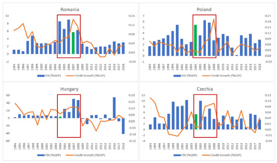
Figure 2.
FDI net inflows (% of GDP) and credit growth to GDP ratio (%). Note: credit growth to GDP ratio is computed as the annual difference in the total credit stock divided by annualized nominal GDP, in order to create a proxy for credit flows and obtain a comparable measure to FDI flows. Source: World Bank Database.
3. Materials and Methods
3.1. Estimating the Elasticity between Economic Growth and Credit
The first step of the analysis employs a naive approach for assessing the relationship between economic growth and credit, by estimating linear regressions. In terms of comparative advantage to other studies focusing on this relationship, we build a dataset using quarterly data spanning from 2004, capturing the early stages of development of the banking sector in the EU accession context, to 2019.
Macroeconomic variables related to real GDP, consumption and investment were extracted from the Eurostat database, while information related to credit, both on an aggregate and sectoral basis were extracted from the central banks websites. The data is transformed into quarterly growth rates for estimating the time varying elasticity coefficients, respectively into yearly growth rates for the cross-correlations and lead-lag relationships. A time-varying specification is chosen to accommodate the higher volatility present in macroeconomic and financial data, especially in the run-up to the Global Financial Crisis.
In order to compute time-varying elasticity coefficients, Bayesian rolling window regressions are estimated, starting from the following standard representation:
In the Bayesian framework, the parameters are not point estimates but conditional posterior densities from which we can extract various moments. Therefore, we define prior distributions, choosing in this case a nature conjugate prior setting in order to obtain an analytical solution for the posterior distribution:
where and are parameters from the Normal distribution for the regression coefficients in , and a and b are shape and scale parameters defining the Inverse Gamma distribution. We draw 10,000 samples from the posterior distribution and compute the median but also plot the kernel densities in order to assess the statistical significance of the results. Moreover, to uncover changes in the time-varying relationship between the real economy and the financial sector, the elasticity coefficients are estimated on a 3-year rolling window (12 quarters).
Complementing the rolling window regression and causality analysis, we add a time dimension and search for the maximum correlation between the series at different lags with the intention of uncovering potential lead-lag relationships. For this purpose, we resort to the sample cross correlation function—which measures the similarity between a time series and lagged versions of another—and the windowed cross-correlation, which computes the statistical measure over iterative “windows” of the sample.
3.2. Using a Structural TVP-SVAR Model to Identify Credit Supply Shocks and Their Role in Explaining Economic Growth
This section details a time-varying parameters SVAR model with stochastic volatility and sign restrictions. Taking into account the higher volatility present in the data warrants employing flexible models incorporating stochastic volatility in order to accurately capture structural relationships. The identification of the credit shocks is achieved using sign restrictions. The numerical computation and optimization procedures were performed in Matlab 2017b [28], using the Bayesian Estimation, Analysis and Regression (BEAR) Toolbox [29] developed by Dieppe et al. [29].
As expressed in Formula (3), the chosen vector autoregressive model (VAR) allows for time variation both in its coefficients and in the residual covariance matrix:
with
and representing the vector of long-term values.
The model described in Formula (4) can also be illustrated as follows:
with
and
where
We resort to the Gibbs sampling algorithm to recover the results of the estimation. The lag length of the model was set to four lags.
The structural shocks’ identification methodology is based on sign restrictions, as described in Table 1, which allows us to avoid the usual recursive assumptions on the contemporaneous effects between endogenous variables. Our assumptions closely follow the traditional identification schemes used in empirical literature, such as in Gambetti and Musso [30] and in the further developed study of Gambetti and Musso [25]. More precisely, we allow for a shock in investment, which drives real GFCF and inflation upwards while also having an expansionary impact on NFC’ credit, while an expansionary NFC credit supply shock has a positive impact on real investment and NFC credit. On the other hand, we impose a negative sign restriction on the short-term interest rate.

Table 1.
Sign restrictions imposed in the TVP-VAR model.
In terms of data, we include variables related to economic activity: the real gross fixed capital formation year-on-year growth rate—a measure of price dynamics—the HICP year-on-year rate, year-on-year growth rate of the exchange rate, a short-term interest rate, namely, the 3-months money market reference rate, and the yearly growth rate of the total stock of loans granted to non-financial corporations. In this regard, we build a dataset using quarterly data spanning from 2005 Q1 to 2019 Q2, capturing the different stages of the financial and business cycles in the four analyzed CEE economies.
Compared to other papers that use the same approach, we included in the model solely the short-term interest rate, as the spreads between the loan interest rates and the short-term interest rate are available only starting 2007, significantly reducing the length of the dataset. We also use the short-term interest rate as a proxy for the credit cost.
4. Results and Discussion
4.1. Estimating the Elasticity between Economic Growth and Credit
The results for the constant and slope extracted from the rolling window regressions (Figure 3), indicate that the relationship between real GDP and total credit growth rates is relatively stable in the pre-crisis period for all the economies included in the study, followed by an increase after 2009. Nevertheless, it is very interesting to notice that Romania, Czechia and Hungary experienced inversion episodes, indicating periods of creditless recovery, when the economic activity was bolstered by measures from other policy areas. According to the slope’s dynamics, the Hungarian economy experienced two such events, both of them lasting for almost two years, with the strongest one covering the Global Financial Crisis and the immediate period after the crisis.
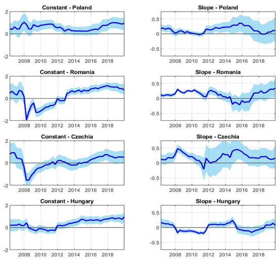
Figure 3.
Results from rolling window Bayesian regressions between economic growth and total credit growth. Note: results are obtained for a rolling window of 3 years (12 quarters) using 10.000 draws of the Gibbs sampler; 95 percent credible sets. Source: own estimations.
More recently, the elasticity coefficient has become positive and is constant or increasing for the selected CEE countries, on the backdrop of lower statistical significance emphasized by the widening of the interpercentile interval. In fact, when assessing the statistical relevance of the series under scrutiny, a high degree of uncertainty is associated with the post 2015 period, for all countries, and therefore, the additional uncertainty surrounding the estimates warrants caution in interpreting the results.
Extending the analysis to the subcomponents, some similarities can be identified together with significant differences. Regarding the case of the consumption–household credit relationship (Figure A1a), the computed rolling window results follow a similar dynamic to their corresponding estimates on economic growth–total credit growth. However, for Czechia and Poland, the results indicate a lower statistical significance. For the case of Romania, the coefficient is mostly positive throughout the entire time span and increases rapidly in the post-crisis period. The conclusions radically change for all the four countries when illustrating the results for investment (Gross Fixed Capital Formation) and non-financial corporations’ credit growth (Figure A1b). First of all, the coefficient is significantly higher than in the case of the previously mentioned estimates, being also accompanied by a strong statistical significance throughout the entire period, for all four countries, potentially underlining the multiplicative effect of credit granted towards productive economic sectors for the real economy.
As a robustness check, we plot the kernel density estimates of the coefficients obtained from the rolling window regressions (Figure A2 and Figure A3a,b). Drawing a general conclusion from the joint analysis of the three pairs of macro and financial variables for all the studied CEE members, statistical significance has dropped significantly after 2010 and, therefore, the additional uncertainty surrounding the estimates warrants caution in interpreting the results. However, the statistical significance remains mostly strong in case of the credit granted to NFC and investment.
Finally, in order to ensure that the results are not distorted by the choice related to the size of the rolling window (12 quarters), we iteratively re-estimate the models using rolling windows from 12 to 24 quarters. Analyzing the results from Figure A4, we can ascertain that, while some changes occur in the dynamics of the series, especially in the period following the Global Financial Crisis, the overall conclusions previously formulated remain largely unchanged.
On average, the results from the sample cross-correlation functions indicate that consumption closely follows household credit (by one or two quarters) for three of the four economies, Hungary being the only exception in this regard. However, the interesting fact highlighted by the above figure is once again the importance of a sustainable supply of credit towards productive sectors in order to support investment, considering the significant time lag estimated for this relationship–credit granted to NFC is leading gross fixed capital formation by 3 quarters in Czechia and Poland and by 2 quarters in Romania and Hungary (Figure 4).
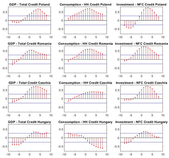
Figure 4.
Sample Cross-correlations estimated for the macro and credit variables. Source: own estimations.
From a visual inspection of the windowed correlation plots (Figure 5) it is clear that, in the case of the aggregate variables, cross-correlations are lower than for the sectoral pairs in the case of Poland and Czechia. We find high degrees of windowed cross-correlations between investment and NFC credit in Poland and between consumption and household credit in Czechia. Furthermore, while all the heat maps exhibit a significant episode overlapping with the onset of the Global Financial Crisis, in the case of the relationship between credit to non-financial corporations and investment, it is visible that the cross-correlations remain strong even in the more recent years.
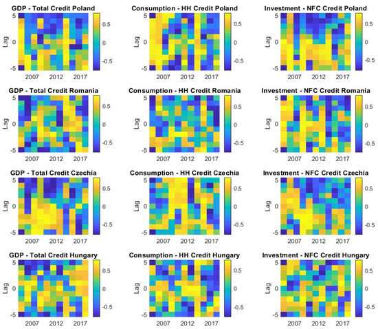
Figure 5.
Windowed Cross-correlations estimated for the macro and credit variables. Source: own estimations.
4.2. Using a Structural TVP-VAR Model to Identify Credit Supply Shocks and Their Role in Explaining Economic Growth
At first, we estimated the constant parameters models, aiming to observe the suitability of the model to the analyzed data. The obtained results indicate a good fit of the chosen model, for all the series. Furthermore, in order assess the robustness of the results we use various prior calibration methods such as the Minnesota prior, the Inverse Wishart prior or the Dummy prior, as defined by Banbura et al. [31].
We identified two shocks: an NFC credit supply shock and a shock in the gross fixed capital formation. Credit supply shocks can be associated with a set of events, such as unexpected changes in bank capital available for loans, changes in bank funding, changes in the risk perception of potential borrowers by bank management or changes in the degree of competition in the banking sector. Figure 6 details the response of credit granted to non-financial corporations to a positive one standard deviation investment shock (left side) and the response of investment to a positive one standard deviation NFC credit shock (right side) in all the four studied economies. Regarding the first one mentioned, the calibration methods indicate a positive effect for all four countries. The duration of the reactions is also similar across most economies, the effect of an investment shock being active for around 12 quarters in Poland, Romania and Czechia and for almost 20 quarters in Hungary. Taking the results of the Bayesian VAR estimated using Minnesota univariate-AR as calibration method, the models indicate a peak in the first three quarters for all countries. The strongest result is identified in Hungary’s case, with a maximum response of 1.51 pp, followed by Romania (1.37 pp), Poland (1.17 pp) and Czechia (0.95 pp). Moreover, comparing the impulse response functions for all the variables included in the country models (Figure A5), it is a clear fact that the strongest positive response is the one of the NFC loan growth to an investment shock, indicating an important effect of the real economy on the financial sector. Therefore, we can ascertain that the investment shock identified in the structural model is in accordance with mainstream literature and brings further evidence to support the model’s robustness.
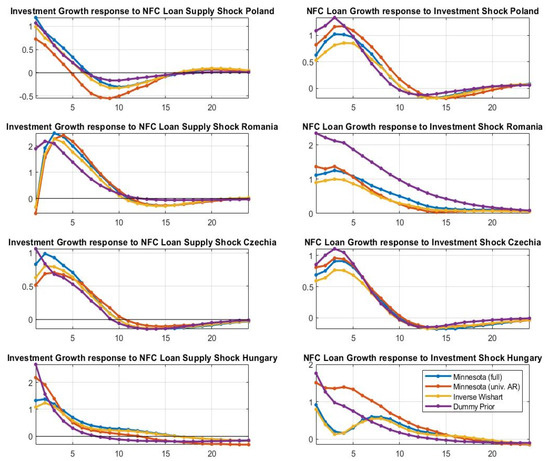
Figure 6.
Impulse response functions to an investment shock and an NFC loan supply shock obtained from BVAR models with sign restrictions using multiple methods for the calibration of priors. Source: own estimations.
Furthermore, Figure 6 illustrates the responses to a positive one standard deviation NFC credit supply shock. All calibration methods indicate very similar effects on investment across the selected CEE countries. For all four economies, the positive response of the investment growth is significant but short lived, returning to baseline more quickly than the previous discussed case; the duration of the effect lasts up to 7 periods in Poland, 10 periods in Romania and Czechia and between 10 and 15 periods in Hungary, depending on the prior calibration choice. However, the strength of the response remains considerably high, with a peak of 2.41 pp for Romania, 2.17 pp for Hungary, 0.72 pp for Poland and 0.70 pp for Czechia. Therefore, according to our results, the effect of an NFC credit supply shock on the investment growth is both smaller and shorter than the effect of an investment shock on the NFC loan growth for Czechia and Poland, while for Romania and Hungary the effect of an NFC credit supply shock on the investment growth is stronger, although shorter.
Moreover, we augment the model with time variation in the coefficients and innovations (Figure 7). Time-varying impulse response functions indicate an amplification in the case of the credit granted to non-financial corporations’ supply shock on the investment growth after 2016, for all the four countries. Both responses remain positive during the analyzed period. Time variation allows for uncovering important structural changes throughout the entire period under scrutiny. Romania and Czechia show very similar patterns, for which we can split the sample into three different subsamples: (i) the first part until 2010 shows a heightened but decreasing response, (ii) the second part, between 2010 and 2016, is the period with the smallest responses and (iii) the post-2016 period shows increasing responses. Heterogeneity and dynamic contributions are consistent with previous empirical results obtained using this methodology, such as Guevara and Rodrigues [26] or Bijsterbosch and Falagiarda [21].
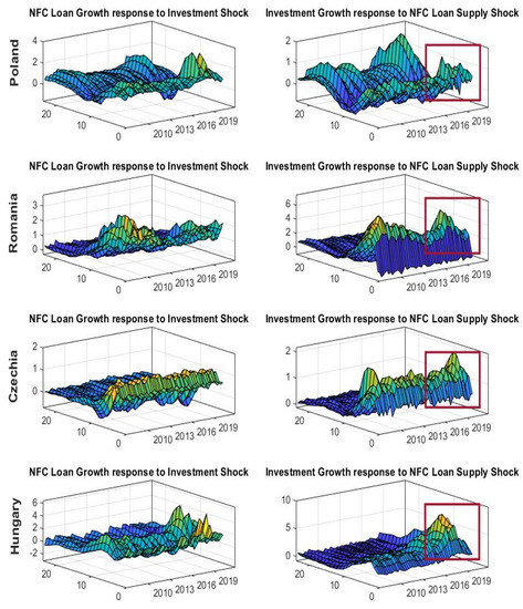
Figure 7.
Time-varying impulse response functions. Source: own estimations.
The latter results hints towards the increasing role of the financial sector and the opportunity of CEE countries to foster a new model of sustainable economic growth, where business cycle volatility can be significantly dampened through countercyclical credit provision.
Analyzing the historical decomposition, a sign change is identified in both contributions at the end of 2008 (Figure A6), for all countries, together with positive peaks in 2008 and negative ones in 2010. Moreover, as already indicated by the impulse response functions, the contribution of the investment shock to the credit growth variation is comparable to the contribution of the NFC loan supply shock to the investment growth variation.
Finally, in order to add a cross-sectional dimension to our analysis of investment and credit supply shocks, we extract the structural shocks for each country and compute pairwise correlation coefficients (Figure 8). We generally find weak correlations between investment shocks in the selected CEE countries, which is not surprising as investment heavily depends on various structural factors specific to each economy, with the exception of Poland and Hungary, signaling the potential of contemporaneous capital movements and common investing strategies by international investors. Similarly, credit supply shocks exhibit a low degree of correlation among the analyzed countries, while Romania and Hungary display the highest correlation coefficient mostly on the backdrop of synchronized credit cycles, with common boom–bust phases and high volatility as compared to other CEE peers.
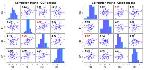
Figure 8.
Correlation matrix of investment and credit supply shocks. Source: own estimations.
5. Conclusions
The present paper provides a comprehensive analysis of the relationship between credit and sustainable economic growth in Poland, Romania, Czechia and Hungary after 30 years of financial sector development. In terms of comparative advantage to other studies focusing on this relationship, we built a dataset using quarterly data spanning from 2004, capturing the early stages of development of the banking sector in the EU accession context, to the second quarter of 2019.
First, using Bayesian regressions, we ascertain that the relationship between real GDP and total credit growth rates is relatively stable in the pre-crisis period for all the CEE countries included in the study, followed by an increase after 2009. More recently, the elasticity coefficient has become positive and is constant or increasing, on the backdrop of lower statistical significance. Nevertheless, Romania, Czechia and Hungary experienced inversion episodes, identified as periods of creditless recovery, when the economic activity was bolstered by measures from other policy areas.
The second part of the paper focuses on a TVP–VAR model with stochastic volatility and sign restrictions, used to identify the role played by NFC credit supply shocks over the main macroeconomic variables in the CEE members considered, using quarterly data spanning from 2004 to 2019, that allows us to capture different stages of the financial and business cycles.
The impulse response functions indicate a significant positive response of the credit granted to non-financial corporations to a positive one standard deviation investment shock. Further, the duration of the reactions is similar across most countries, the effect of an investment shock being active for around 12 quarters in Poland, Romania and Czechia and for almost 20 quarters in Hungary. On the other hand, the response of the investment to a positive one standard deviation NFC credit supply shock remains for positive for all countries, but short-lived, returning to baseline more quickly than the previous discussed case. According to our results, the effect of an NFC credit supply shock on the investment growth is both smaller and shorter than the effect of an investment shock on the NFC loan growth for Czechia and Poland, while for Romania and Hungary the effect of an NFC credit supply shock on the investment growth is stronger, although shorter.
Time-varying impulse response functions indicate an amplification in the case of the credit granted to non-financial corporations’ supply shock on the investment growth after 2016, in the selected CEE countries. Both responses remain positive during the analyzed period. Time variation allows us to uncover important structural changes throughout the entire period under scrutiny. Romania and Czechia show very similar patterns, for which we can split the sample into three different subsamples: (i) the first part until 2010 shows a heightened response but decreasing, (ii) the second part, between 2010 and 2016, is the period with the smallest responses and (iii) the post-2016 period shows increasing responses. The latter results hints towards the increasing role of the financial sector and the opportunity of CEE countries to foster a new model of sustainable economic growth, where business cycle volatility can be significantly dampened through countercyclical credit provision.
Potential policy solutions to ensure a sustainable contribution of the financial sector to economic growth relate to the strong relationship identified between investment and loans granted to non-financial corporations. In this sense, the leading behavior of non-financial corporations’ credit growth coupled with the statistically significant and high elasticity coefficient support the conclusion that credit plays an important role in driving investment, with positive repercussions of ensuring a sustainable rate of economic growth.
Starting from the strong relationship between investment and non-financial companies’ loans, potential policy measures to ensure sustainability require a long-term investment perspective, with a strong focus on green finance and less carbon intensive economic sectors. From a policy-making perspective, higher costs related to changing the short-term perspective related to sustainable finance could require relaxing regulation through lower requirements for green loans or subsidies and state guarantees for financing transition towards less carbon intensive economic sectors.
A future direction to our research relates to studying the implications of financial inclusion on sustainable growth and to assess the relationship between green financing and economic growth, once time series become available.
Author Contributions
Conceptualization, A.A., M.N.K. and A.Z.; methodology, A.A. and M.N.K.; software, M.N.K. and A.Z.; validation, A.A., M.N.K. and A.Z.; formal analysis, A.A.; investigation, M.N.K.; resources, A.Z.; data curation, A.A.; writing—original draft preparation, A.Z.; writing—review and editing, A.A. and M.N.K.; visualization, A.Z.; supervision, A.A.; project administration, M.N.K. and A.Z. All authors have read and agreed to the published version of the manuscript.
Funding
This research received no external funding.
Institutional Review Board Statement
Not applicable.
Informed Consent Statement
Not applicable.
Data Availability Statement
The macroeconomic variables included in the study were extracted from the Eurostat database: https://ec.europa.eu/eurostat/web/main/data/database, accessed on 25 March 2020; the information related to credit, both on an aggregate and sectoral basis, were extracted from the central banks websites, as follows: National Bank of Romania: https://www.bnr.ro/Interactive-database-1107.aspx, accessed on 28 March 2020, Czech National Bank: https://www.cnb.cz/en/statistics/, accessed on 28 March 2020, Magyar Nemzeti Bank: https://www.mnb.hu/en/statistics, accessed on 28 March 2020, Narodowy Bank Polski: https://www.nbp.pl/homen.aspx?f=/en/statystyka/statystyka.html, accessed on 28 March 2020; data related to global economic growth and financial intermediation, as well as data related to FDI net inflows (% of GDP) and credit growth to GDP ratio (%) were extracted from the World Bank database: https://data.worldbank.org/, accessed on 12 April 2020.
Conflicts of Interest
The authors declare no conflict of interest.
Appendix A

Figure A1.
(a) Results from rolling window Bayesian regressions between consumption and households’ credit; (b) Results from rolling window Bayesian regressions between investment growth and non-financial corporations’ credit. Note: results are obtained for a rolling window of 3 years (12 quarters) using 10,000 draws of the Gibbs sampler. Source: own estimations.

Figure A2.
Posterior densities of estimated coefficients from the Bayesian regressions on GDP and total credit. Source: own estimations.

Figure A3.
(a) Posterior densities of estimated coefficients from the Bayesian regressions on consumption and households’ credit; (b) Posterior densities of estimated coefficients from the Bayesian regressions on investment and non-financial corporations’ credit. Source: own estimation.

Figure A4.
Bayesian regression estimation results on GDP and total credit using recursive rolling windows between 12–24 quarters. Note: colors range from dark blue (12 quarters) to dark red (24 quarters). Source: own estimations.
Appendix B


Figure A5.
Impulse response functions obtained from BVAR with sign restrictions using multiple methods for the calibration of priors. Source: own estimation.


Figure A6.
Historical Decomposition. Source: own estimation.
References
- Claessens, S.; Kose, M.A.; Terrones, M.E. Financial cycles: What? How? When? NBER Int. Semin. Macroecon. 2017, 7, 303–344. [Google Scholar] [CrossRef]
- Schumpeter, J.A. A Theory of Economic Development; Harvard University Press: Cambridge, MA, USA, 1911. [Google Scholar]
- Goldsmith, R.W. Financial Structure and Development; Yale University Press: New Haven, CT, USA, 1969. [Google Scholar]
- McKinnon, R.I. Money and Capital in Economic Development; The Brookings Institution: Washington, DC, USA, 1973. [Google Scholar]
- Shaw, E.S. Financial Deepening in Economic Development; Oxford University Press: New York, NY, USA, 1973. [Google Scholar]
- Robinson, J. The Rate of Interest and Other Essays; Macmillan: London, UK, 1952. [Google Scholar]
- Lucas, R. On the mechanics of economic development. J. Monet. Econ. 1988, 22, 3–42. [Google Scholar] [CrossRef]
- Paun, C.V.; Musetescu, R.C.; Topan, V.M.; Danuletiu, D.C. The Impact of Financial Sector Development and Sophistication on Sustainable Economic Growth. Sustainability 2019, 11, 1713. [Google Scholar] [CrossRef]
- Petkosky, M.; Kjosevski, J. Does Banking Sector Improve Economic Growth? An Empirical Analysis for Selected Countries in Central and South Eastern Europe. Econ. Res. Ekon. Istraz. 2014, 27, 55–66. [Google Scholar]
- Loayza, N.; Ouazad, A.; Ranciere, R. Financial Development, Growth, and Crisis Is There a Trade-Off? Policy Research Working Paper 8237; World Bank Group, Development Research Group, Macroeconomics and Growth Team: Washington, DC, USA, 2017; pp. 1–40. [Google Scholar]
- Faust, J. The robustness of identified VAR conclusions about money. In Carnegie Rochester Conference Series on Public Policy 49; Springer: Berlin/Heidelberg, Germany, 1998; pp. 207–244. [Google Scholar]
- Canova, F.; De Nicolo, G. Monetary disturbances matter for business fluctuations in the G-7. J. Monet. Econ. 2002, 49, 1131–1159. [Google Scholar] [CrossRef]
- Uhlig, H. What are the effects of monetary policy on output? Results from an agnostic identification procedure. J. Monet. Econ. 2005, 52, 381–419. [Google Scholar] [CrossRef]
- Bean, C.; Paustian, M.; Penalver, A.; Taylor, T. Monetary Policy after the Fall, Paper Presented at the Jackson Hole Economic Policy Symposium; Bank of England: London, UK, 2010. [Google Scholar]
- De Nicolo, G.; Lucchetta, M. Systemic Risks and the Macroeconomy; NBER Working Paper: Cambridge, MA, USA, 2011; p. 16998. [Google Scholar]
- Meeks, R. Do credit market shocks drive output fluctuations? Evidence from corporate spreads and defaults. J. Econ. Dyn. Control 2012, 36, 568–584. [Google Scholar] [CrossRef]
- Hristov, N.; Hulsewig, O.; Wollmershauser, T. Loan Supply Shocks during the Financial Crisis: Evidence for the Euro Area. J. Int. Money Financ. 2012, 31, 569–592. [Google Scholar] [CrossRef]
- Barnett, A.; Thomas, R. Has Weak Lending and Activity in the United Kingdom Been Driven by Credit Supply shocks? Manch. Sch. 2014, 82, 60–89. [Google Scholar] [CrossRef]
- Lubik, T.; Matthes, C. Time-Varying Parameter Vector Autoregressions: Specification, Estimation and an Application. Econ. Q. 2015, 101, 323–352. [Google Scholar]
- Bijsterbosch, M.; Falagiarda, M. Credit Supply Dynamics and Economic Activity in Euro Area Countries. A Time-Varying Parameter VAR Analysis; ECB Working Paper, No. 1714; ECB: Frankfurt, Germany, 2014. [Google Scholar]
- Bijsterbosch, M.; Falagiarda, M. The macroeconomic impact of financial fragmentation in the euro area: Which role for credit supply? J. Int. Money Financ. 2015, 54, 93–115. [Google Scholar] [CrossRef]
- Cogley, T.; Sargent, T.J. Drifts and volatilities: Monetary policies and outcomes in the post WWII US. Rev. Econ. Dyn. 2005, 8, 262–302. [Google Scholar] [CrossRef]
- Primiceri, G.E. Time varying structural vector autoregressions and monetary policy. Rev. Econ. Stud. 2005, 72, 821–852. [Google Scholar] [CrossRef]
- Gerali, A.; Neri, S.; Sessa, L.; Signoretti, F.M. Credit and banking in a DSGE model of the euro area. J. Money Credit Bank. 2010, 42, 107–141. [Google Scholar] [CrossRef]
- Gambetti, L.; Musso, A. Loan supply shocks and the business cycle. J. Appl. Econom. 2017, 32, 764–782. [Google Scholar] [CrossRef]
- Guevara, C.; Rodríguez, G. The Role of Loan Supply Shocks in Pacific Alliance Countries: A TVP-VAR-SV Approach. N. Am. J. Econ. Financ. 2020, 52, 101140. [Google Scholar] [CrossRef]
- Avouyi-Dovi, S.; Labonne, C.; Ray, S. Insight from a Time-Varying VAR Model with Stochastic Volatility of the French Housing and Credit Markets; Banque de France Working Paper #620; Banque de France: Paris, France, 2017. [Google Scholar]
- MATLAB 2017b, [Computer Software], Natick; The MathWorks, Inc.: Natick, MA, USA, 2017.
- Dieppe, A.; Legrand, R.; van Roye, B. The BEAR Toolbox; ECB Working Paper, No. 1934; ECB: Frankfurt, Germany, 2016. [Google Scholar]
- Gambetti, L.; Musso, A. Loan Supply Shocks and the Business Cycle; ECB Working Paper Series, No. 1469; ECB: Frankfurt, Germany, 2012. [Google Scholar]
- Banbura, M.; Giannone, D.; Reichlin, L. Large Bayesian vector autoregressions. J. Appl. Econom. 2010, 25, 71–92. [Google Scholar] [CrossRef]
Publisher’s Note: MDPI stays neutral with regard to jurisdictional claims in published maps and institutional affiliations. |
© 2021 by the authors. Licensee MDPI, Basel, Switzerland. This article is an open access article distributed under the terms and conditions of the Creative Commons Attribution (CC BY) license (https://creativecommons.org/licenses/by/4.0/).