Cost Analysis of a Novel Method for Ecological Compensation—A Study of the Translocation of Dead Wood

Abstract

Translocation of dead wood is a novel method for ecological compensation and restoration that could, potentially, provide a new important tool for biodiversity conservation. With this method, substrates that normally have long delivery times are instantly created in a compensation area, and ideally many of the associated dead wood dwelling organisms are translocated together with the substrates. However, to a large extent, there is a lack of knowledge about the cost efficiency of different methods of ecological compensation. Therefore, the costs for different parts of a translocation process and its dependency on some influencing factors were studied. The observed cost was 465 SEK per translocated log for the actual compensation measure, with an additional 349 SEK/log for work to enable evaluation of the translocation’s ecological results. Based on time studies, models were developed to predict required work time and costs for different transportation distances and load sizes. Those models indicated that short extraction and insertion distances for logs should be prioritized over road transportation distances to minimize costs. They also highlighted a trade-off between costs and time until a given ecological value is reached in the compensation area. The methodology used can contribute to more cost-efficient operations and, by doing so, increase the use of ecological compensation and the benefits from a given input.

1. Introduction

Anthropogenic disturbance has altered ecosystems worldwide, resulting in habitat loss and species extinctions over a wide range of biomes [1,2]. Forest ecosystems are no exception, and their exploitation has led to changes in ecosystem structures and processes, and to biodiversity loss [2,3]. Species associated with dead wood (saproxylic species) are especially vulnerable.

To conserve biodiversity and continue economic development simultaneously is a major challenge as human society depends on functional ecosystems in numerous ways [4]. Economic growth and biodiversity conservation are often perceived to be incompatible. There is continually increasing pressure on corporations by consumers and stakeholders to be environmentally conscious with greater focus being directed towards alternative approaches in adapting to this [5]. One such approach is the relatively recent concept of ecological compensation (biodiversity offsetting), which is based on the principle that those who destroy or damage natural values are to compensate for this by the creation or protection of natural values at a different/substitute location [6]. Thus, ecological compensation potentially provides an approach that links biodiversity conservation and human development associated with economic growth. Although legislation mandating biodiversity offsets exist in many countries at present, biodiversity offsets are still under development.

Biodiversity offsets are the last step in the mitigation hierarchy, with the overarching goal to achieve no net loss of biodiversity [6]. These actions can involve protection of areas that are otherwise at risk of exploitation, through ecological restoration or other positive management interventions and, in some circumstances, the re-creation of habitat that has been lost. Restoration of degraded habitat is often used for ecological compensation and, although our knowledge of the effects of different restoration methods on biodiversity has improved in recent years [7,8,9,10], it often suffers from the innate problem that even if substrates or habitat for species that we want to favor are provided, those species may not be able to migrate to the restored areas [7,9]. Furthermore, the delivery time of some types of substrates is long, e.g., large diameter dead wood takes a very long time to develop and reach late decompositions stages, and it could take centuries after restoration before these kind of substrates are available for specialist species. One way to circumvent this problem is the translocation of substrates and associated species from the impact area to compensation areas.

Translocation means that habitats and substrates with long delivery times are instantly created in a compensation area. In addition, in the best-case scenario, many of the organisms associated with these high-quality substrates are translocated together with the substrates rather than having to migrate there. Thus, fulfilment of the “fields of dreams” hypothesis would be unnecessary for successful compensation and/or restoration [11].

Due to the concept of ecological compensation being a novel one, there is little in the way of relevant research on methods and outcomes of ecological compensation. However, there have been assessments of the ecological functionality and methods for evaluation of the compensation measures (e.g., [12]), and also research into the social and economic effects on local societies (e.g., [13]). However, there has been limited focus on the costs of carrying out the actual compensation measures. When such costs have been investigated, it has often been in terms of the total costs for compensation projects carried out, with little focus on comparing alternatives in order to find and develop cost-efficient practices (e.g., [14]). Even when the ecological compensation constitutes a minor part of large-scale projects, such as the construction of roads and establishment of mines, cost-efficiency is, nevertheless, instrumental for increasing both the use of ecological compensation and increasing the benefits from a given economic input.

Evaluation of cost-efficiency is a central part of research in, for example, forest operations. Based on methods for cost assessment, such research focuses on evaluations of, and improvements to, work carried out, and on predicting the outcomes of planned operations. The aim is to estimate the cost of the work required to produce the desired outcome of the operation. To do so, the cost assessment focuses on two main parts: the cost per unit of time, and the time required per produced unit. The cost per time unit is based on the labor costs, operational costs and investment costs related to the operation [15]. The time required per produced unit is often called time consumption, and often there is a focus on the inverse of the time consumption—the productivity (produced units per time). The time consumption is dependent on the conditions in which the operations are carried out and is measured by dividing the work into distinct parts (work elements) in order to isolate influencing factors better. By doing so, relationships between time consumption and the influencing factors are easier to distinguish [16]. There is a wealth of research on time consumption and productivity of conventional forest operations, with well-known general relationships. For instance, the required time consumption per produced unit increases with transport distance and decreases with the number of units that can be handled at a given time (e.g., per load) [17,18,19,20]. Cost-based evaluations of conventional operations are common [21], and there have also been evaluations of how ecological considerations influence the costs of operations [22]. However, cost-based evaluations of ecological compensation are scarce.

The largest copper mine in Sweden is the Aitik mine, founded in 1968 by the mining company Boliden AB. The ore extraction process at the mine produces 50,000 tons of tailings daily. These are subsequently transported to a sand magazine. Recently, the Boliden AB was granted a permit to increase the sand storage area in the Aitik mine by 376 ha. The affected forest land had high to very-high natural value and The Land and Environmental Court of Appeal decided that offsets areas should be created to compensate for the impact. In addition, as part of the compensation measures it was decided that substantial amounts of dead wood and associated species of insect, wood fungi, lichens, bryophytes and lichens living in or on the dead wood should be translocated from the impact to a 397 ha compensation area 5 km (in a straight line) west-southwest from the affected area.

The aim of this study was to assess the cost of translocating dead wood from an affected area to the compensation area. More specifically, the focus was on assessing the costs for different parts of the translocation process and their dependency on some influential factors (i.e., transportation distances and load sizes). Moreover, being part of a scientific project to evaluate the ecological outcome of the translocation, the study also provided input on some of the costs associated with carrying out such an evaluation.

This project is unique in its usage of translocation of natural values as a primary means of ecological compensation in boreal forests. The results presented here are thus highly significant for future endeavors involving ecological compensation (in a boreal setting) and may be valuable to other companies facing similar challenges.

2. Materials and Methods

The study was conducted during the creation of off-set areas required to compensate for the impact of increasing the sand storage area in the Aitik mine. Hence, it was an observational study (and not an experimental study), with only limited possibilities to interfere with the work in order to collect desired data.

2.1. Work Phases

The translocation of dead wood consisted of seven phases, from the identification of substrates (phases 1 and 2) to the translocating work (phases 3–7) (Figure 1). All phases, except the log marking, were necessary for the actual translocation work. However, for the area identification, felling and the insertion phases, there was extra work carried out in order to facilitate the planned scientific evaluation of the translocation.

The machine operators who carried out the work in the phases Extraction, Road transport and Insertion were given instructions to drive as normal, but to handle the logs with additional care since they could be more fragile than newly harvested and fresh logs.

2.2. Area Description

The impact and compensation areas are located in the north boreal vegetation zone [23] (Ahti et al. 1968). The area had previously been under silvicultural management, predominantly subjected to selective felling, but had not been managed over recent decades. The forests were dominated by conifers (Scots pine (Pinus sylvestris) and Norway spruce (Picea abies)), and with scattered broadleaves (mainly Downy birch (Betula pubescens)).

The affected area covered 376 hectares, of which 167 hectares consisted of forests of high or very high conservation value as defined by Swedish Standards Institute [24]. The area included 21 red-listed species and forest structures important for biodiversity (e.g., very large old trees, snags and logs of unusual dimensions).

The compensation area covered 397 hectares, of which 192 hectares was productive forest (mean annual increment of at least 1 m³ per ha and year) with high conservation value, 113 hectares of productive forest with low conservation value but with no forest of very-high conservation value. The remaining areas were non-productive forest, mires or open water [25].

To allow for a scientific assessment of the outcome of the translocation of the dead wood for biodiversity, the whole compensation area was systematically inventoried prior to translocation of the dead wood. Thirty circular plots were randomly distributed in areas with productive forest. The translocated dead wood was placed in the plots to enable the planned scientific evaluation. The evaluation focused on assessing ecological effects due to the quality and quantity of dead wood. Hence, each plot received either 48, 16 or zero translocated logs, with 10 replications of each log concentration, giving a total of 30 experimental plots. For each concentration there were instructions on the number of logs of the different types to be placed in each plot. Plots were 50 m in diameter and separated from each other by at least 150 m. Detailed information on the scientific evaluation can be found in [26].

The inventory work and establishment of the plots were carried out by two nature value consultants, who were also involved in work phases 2, 4 and 7.

2.3. Substrate Identification

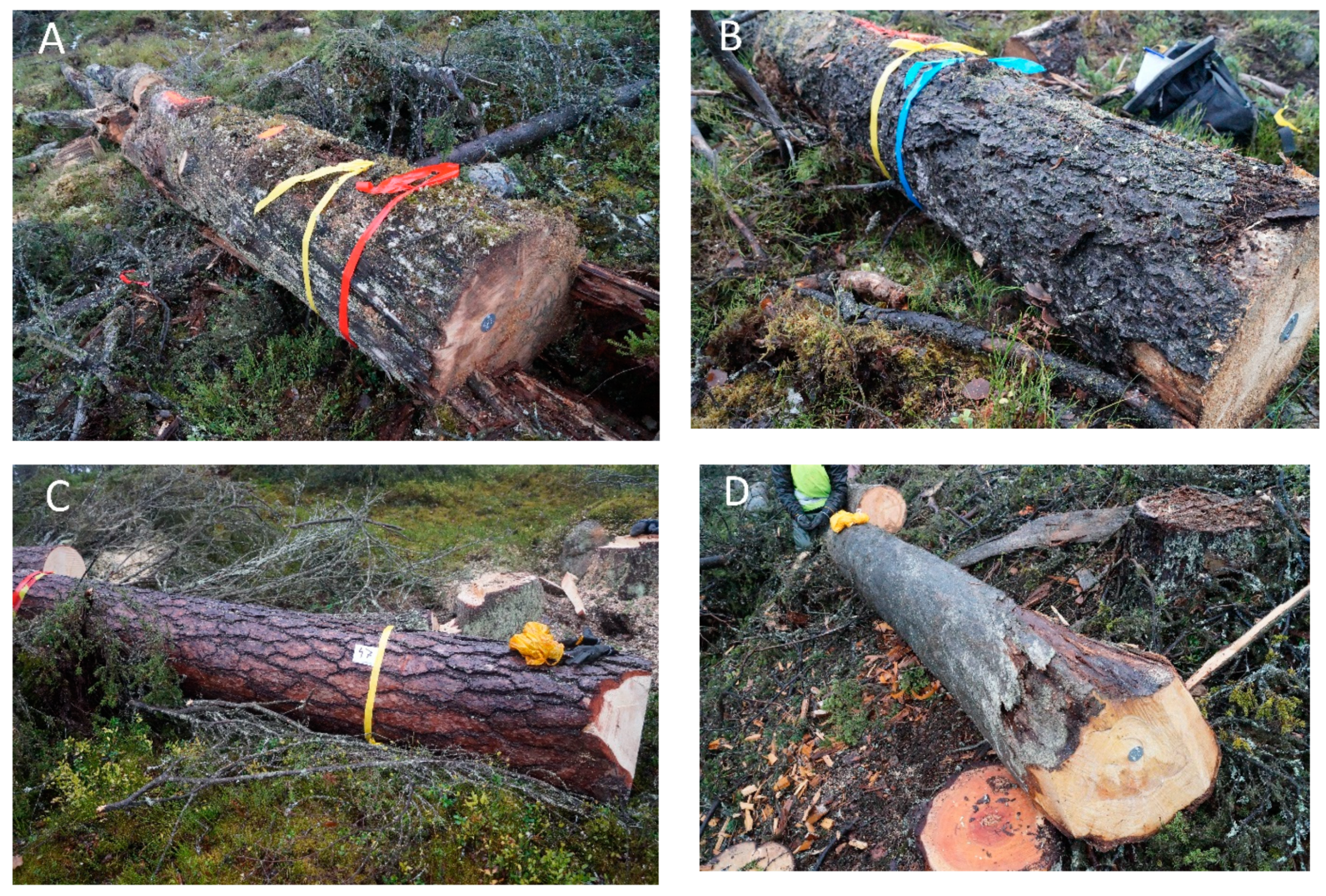
The impact area was systematically inventoried by the nature value consultants for standing and lying trees, and the meeting of criteria for any of the eight log assortments identified based on tree species (Scots pine or Norway spruce), posture (standing or downed) and decomposition stage (fresh, early or intermediate) as suitable for translocation (

Table 1. Log assortments that were translocated, and the mean log volume in each assortment, from sampling carried out for this study.

Species	Posture of Tree	Decomposition Stage	Translocated Logs	Sampled Logs		Log Volume (m3)
			N	n	(%)	Mean	SD
Spruce	Downed	Early decomposition	80	16	20	0.13	0.05
		Intermediate decomposition	80	27	34	0.15	0.05
	Standing	Kelo type (intermediate decomp.)	80	26	33	0.18	0.08
		Fresh	80	17	21	0.33	0.12
Pine	Downed	Early decomposition	20	11	55	0.15	0.07
		Intermediate decomposition	66	15	23	0.23	0.12
	Standing	Kelo type (intermediate decomp.)	94	23	24	0.27	0.13
		Fresh	140	20	14	0.47	0.16
		All pooled	640	155	24	0.24	0.15

, examples in Figure 2). Trees meeting the criteria were marked.

2.4. Tree Felling and Log Marking

The translocation work began on 2 October 2017, starting with felling of standing trees, cutting felled and lying trees to logs and marking the logs. The nature value consultants chose which of the marked trees to create logs from, and to which dimensions. The objective was to find logs with diameters greater than 15 cm and lengths between 3 and 5 m. Some trees marked in the previous phase were excluded from translocation as they were too decayed or too thin. Only dead wood substrates that were considered feasible to move without breaking were selected for the translocation. The number of relocation logs created per tree was not recorded, but the number of logs was just slightly higher than the number of trees marked during the substrate identification phase (Table 4).

The felling and cross-cutting work was carried out by two chainsaw operators, each with at least 25 years of experience in motor-manual forestry operations. Both used Husqvarna 550XPG chainsaws with 25.72 cm (18 inch) blades.

The logs were carefully handled so as not to reduce their value to the project e.g., by not disturbing the attached fruiting bodies of wood fungi. The logs were inventoried for red-listed or indicator species, tagged for dead wood assortment, photographed, and their upper side marked with paint so that they could be placed in the same position after translocation. Finally, they were marked with a unique ID. A total of 671 logs were created. Due to a limited number of lying dead pine trees, with only 20 early and 66 intermediary decomposition logs found instead of the desired 80 in each class, they were supplemented with logs from the pine fresh wood and pine kelo style classes, respectively (see N in Table 1).

2.5. Extraction

All 671 marked logs were extracted from the affected area to the roadside, using a conventional forwarder (

Table 2. Specifications for the machines used for the work phases Extraction, Road Transport and Insertion.

Feature	Extraction	Road Transport	Insertion
Machine type	Forwarder	Self-loading timber truck	Forwarder
Make and model	Komatsu 865	Scania R440	Terri ATD
Manufacturing year	2013	2012	2001
Work time (hours)	10,800	-	4000
Driven distance (km)	-	850,000	-
Laden mass (tonnes a)	18	19.6	3
Width (m)	3.2	2.6	1.8
Length (m)	10	22	6.5–7.1
Load capacity (m3sob)	15	50	4
Propulsion	Wheels with bogie band	Wheels	Tracks
Crane model	CRF 11c	FTG V13	Mowi 2046
Crane reach (m)	12	8	4.6

^a metric tonnes (1 tonne = 1000 kg).

). The size of the forwarder and its impact on the ground was not considered when the machine was being chosen, since the area was to be converted. Logs were arranged by assortment type at two separate landings. In order to protect the translocation logs, the bottom of the pile was made from a layer of conventional roundwood. The extraction was carried out by a machine operator with 18 years of experience of forwarding work.

2.6. Road Transport

The extracted logs were transported using a conventional timber truck (Table 2) from the affected area to three separate landings at the compensation area. The first load (4 logs per assortments, 32 logs in total) was transported to the first landing, loads 2 and 3 were transported to the second landing (28 per log assortment, 224 logs in total) and loads 4,5 and 6 were transported to the third landing (48 per log assortment, 384 logs in total). The logs were loaded in order of decreasing durability, with fresh wood being placed at the bottom, then kelo type trees, early lying dead wood and, finally, intermediate lying dead wood. In total, 640 of the 671 logs were transported, with the numbers per assortments reported in Table 1.

The road transport was carried out by two machine operators with at least 18 years of experience with self-loading timber trucks.

2.7. Insertion

The insertion of logs to the compensation area was carried out using a small tracked forwarder (Table 2) under the supervision of nature value consultants. The size of the forwarder was chosen to minimize the impact on the ground, and so that it could navigate between the trees in the stand. A total of 640 logs were inserted in 20 plots, with 2 logs of each log assortment placed at each of 10 (16 logs per plot) of the 20 plots, and 6 logs of each log assortment at each of the remaining 10 plots (26 logs per plots). Within plots, log assortments were randomly distributed.

The insertion was carried out by two machine operators with 3 and 5 years of part-time experience, respectively, with small forwarders.

2.8. Cost Assessment

Costs were collected in the national currency Swedish krona (SEK), which at the time of the study had an exchange rate of ca 10.0 SEK per Euro and 8.6 SEK per USD.

The total cost for the compensation project was calculated by totaling the total costs for each work phase. The total cost for each work phase was calculated by multiplying the times required to carry out the work involved in the phase by the hourly cost for the respective work.

Cost per translocated log was calculated for each work phase by dividing the total cost for the work phase by the number of translocated logs according to:

$$C_x=\frac{{{\displaystyle \sum }}^{ }\left(T_i\times c_i\right)}{O}$$

(1)

where C is the cost per translocated log for work phase x, T is the time required for work i in the work phase, and c is the hourly cost for work i. O is the number of translocated logs (irrespective of the number of objects handled in work phase x).

For the phases Extraction, Road Transport and Insertion, the work was assessed in more detail by use of time studies in order to enable the creation of models for cost estimations under various work conditions, i.e., with time requirements other than the observed total time requirements in this study.

2.9. Time Studies

The work-time required for translocation, divided into the different work phases, was collected from the self-reported work-time of the operators. For the three last phases (Extraction, Road transport and Insertion) detailed time studies conducted on site were carried out on a number of loads.

For the studied loads, total values of load size, time consumption and distance driven were recorded. Driving speeds were derived from distance and time recordings. The time consumption per observed load in the phases was recorded, split over six work elements (

Table 3. Definition of work elements used in this study.

Work Element	Definition
Loading	From the first log being gripped to the last log being put in the loadspace
Driving full	From the last log being put in the loadspace to the first log being gripped for unloading
Unloading	From the first log being gripped for unloading to the last log being put on the ground
Driving empty	From the last log being put on the ground to the first log being gripped for loading
Miscellaneous	Work-related activities that fit into none of the above work elements
Delay	Non-work-related disturbances (phone calls, machine breakdowns, etc.)

) to isolate influential variables. Extraction was the first work phase to be time studied and suffered from initial technical challenges to record the driving distances. Hence, between 9–11 of the 26 loads were properly recorded with driving distances at work element level (see “n” under Transport distance in Table 6).

The work element Loading was observed at even higher resolution for the Road Transport and Insertion phases, by recording loading time per log assortment. In addition to time, distances driven, load sizes (number of logs) and number of crane cycles (loading/unloading) were also recorded.

During extraction, loading times per log assortment were not recorded, since the logs were loaded in the order they were found in the forest, which was not organized by log assortment. Furthermore, it was difficult to determine when the work element Loading was complete, due to the variation in load capacity usage and the indistinct loading area (i.e., loading both when driving from and to the landing).

All time studies were carried out by the same person. During Extraction and Road Transport, the person was located in the machine cabins and, for the Insertion, the person followed the forwarder on foot. The time consumption by the time studies work was recorded in units of a second.

2.10. Calculations

Speed was calculated as the distance driven divided by the time consumption for the work element and/or load (round trips) of interest. Productivity, here defined as the output (in terms of logs or m³) per time unit, was calculated as the load size divided by the time consumption for the work element and/or load (round trips) of interest of the respective work element.

Between 14 and 55% of the logs in the eight translocated log assortments were sampled to give volume estimations (Table 1). Individual log volumes were calculated assuming a cylinder:

$$(V=\frac{\pi *d^2}{4}\times l)$$

(2)

where V is the volume, d is the log diameter over bark at half-length and l is the full length of the log. Hence, an even tapering of the logs was assumed. The volume unit used was solid cubic meter of wood over bark (m³).

Load sizes during Extraction, Road Transport and Insertion were calculated as the total volume of logs in the load, by multiplying the load’s number of logs of each log assortment with the mean log volume for each log assortment (i.e., from Table 1). Utilized load capacity was calculated by dividing load size by the machine’s load capacity (Table 2).

2.11. Statistical Analysis

The impact of transport distance and load size during the work phases Extraction, Road transport and Insertion, on the time consumption of work elements Loading, Driving Full, Unloading and Driving empty, was assessed using linear regression. Data preparation was carried out using Microsoft Excel, whereas all the regression analyses were carried out using Minitab 17 (Mintab Inc., State College, PA, USA) with the critical significance level set to 5%.

3. Results

The results are here presented in three levels of detail. First, the work phase costs are reported, based on the costs invoiced. Second, detailed analysis of the work carried out with some work phases is reported, along with the analysis of the relationships between work time required and work conditions. Third, those relationships are used to model estimated costs under other conditions, in order to highlight cost-driving factors as well as to demonstrate the possibility of using the analysis to estimate costs for future projects.

3.1. Costs

The total costs of the seven work phases involved in the compensation project was 520,800 SEK (

Table 4. Time consumption, hourly cost, total cost, number of objects (logs/trees), cost per translocated log (n = 640) and the work phases’ proportion of the cost.

Work Phase	Work Time including Actions Driven by		Time Consumption (hours)	Hourly Cost (SEK/hour)	Total Cost (SEK)	Number of Objects	Cost per Translocated Log (SEK/log)	Proportion of Cost (%)
	Compensation	Evaluation
Area identification	Yes	Yes	60	525	31,500	-	49.2	6
Substrate identification	Yes	No	90	525	47,250	600	73.8	9
Felling	Yes	Yes	240	400	96,000	671	150.0	19
Log marking	No	Yes	240	525	126,000	671	196.9	24
Extraction	Yes	No	47.5	900	42,750	671	66.8	8
Road transport	Yes	No	27	900	24,300	640	38.0	5
Insertion total			240	637.5	153,000	640	239.1	29
Insertion of logs	Yes	Yes	120	750	90,000	640	140.6	17
Natural value consultant(s) at insertion	No	Yes	120	525	63,000	640	98.4	12
Total			884.5		520,800	640	813.8	100

). When distributing the total costs over the number of translocated logs, the cost per log was 813.8 SEK. The insertion of logs to the plots in the compensation area was the most expensive work phase, accounting for around 29% of the costs. About two thirds of the insertion cost was associated with the physical translocation of logs, while one third pertained to the work of the nature value consultants. The cheapest work phase was the Road Transport, which accounted for 5% of the costs.

The cost for work directly related to the planned scientific evaluation of the ecological compensation project was made up of all log marking, all of the nature value consultants’ contribution at insertion, 20 h (33%) of the time consumption for area identification, 6 h (5%) of the time for insertion of logs (i.e., 20% of the unloading time, see time required below) and 40 h (20%) of the tree felling. When totaling those times and the related hourly cost, the cost related to carrying out the scientific evaluation was 348.8 SEK per log and the cost for the actual compensation work was 465.0 SEK/log. Hence, the included operational preparations for the scientific evaluation of the project required an additional 75% of financial resources, in addition to the resources needed for the compensation work.

3.2. Work Analysis

On average, 18 logs were put on each load during extraction, which was almost twice as many as when inserting the logs (

Table 5. Load sizes and logs per crane cycle for the work phases Extraction, Road Transport and Insertion.

Feature	Extraction			Road Transport			Insertion
	n	Mean	SD	n	Mean	SD	n	Mean	SD
Load size (Number of logs)	26	18.4	6.1	6	106.7	48.75	17	10.4	3.8
Load size (m3)	26	5.1	2.3	6	28.6	11.6	17	2.8	0.6
Utilized load capacity (%)	26	34	15	6	57	23	17	69	16
Logs per crane cycle at loading (n)	26	0.98	0.06	6	2.14	0.43	17	1.02	0.09
Logs per crane cycle at unloading (n)	25	1.02	0.09	6	2.38	0.29	17	1.00	0.00

). However, in terms of utilization of the different vehicles’ payload capacities, the conditions were reversed. In fact, only one third of the payload capacity was, on average, used during extraction, whereas more than two thirds were used during insertion. This was due to a much smaller payload capacity on the forwarder used for insertion (Table 2).

Logs were generally loaded and unloaded individually during the extraction and insertion, whereas slightly more than two logs were handled at a time when loading and unloading during road transport (Table 5).

On average, the total distance driven during Extraction was almost 1.6 km per load, 49 km during Road Transport, and 2.3 km during Insertion (

Table 6. Time consumption, transport distance and speed per load for the four work phases, distributed over work elements.

Work Phase	Work Element		Time Consumption per Load (h)			Transport Distance per Load (km)			Speed per Load (km/h)
		n	Mean	SD	n	Mean	SD	n	Mean	SD
Extraction	Driving empty	26	0.15	0.10	11	0.32	0.19	11	2.35	0.34
	Loading	26	0.38	0.20	10	0.39	0.27	10	1.20	0.35
	Driving full	26	0.12	0.10	9	0.20	0.16	9	2.15	0.44
	Unloading	26	0.14	0.06	10	0.07	0.05	10	0.49	0.30
	Miscellaneous	26	0.03	0.04	-	-	-	-	-	-
	Delay	26	0.05	0.10	-	-	-	-	-	-
	All pooled 1	26	0.87	0.45	24	1.57	0.94	-	-	-
Road transport	Driving empty	6	0.63	0.32	6	25.3	13.48	6	40.0	2.78
	Loading	6	0.83	0.40	6	0.71	0.83	6	0.77	0.69
	Driving full	6	0.59	0.27	6	22.9	10.88	6	38.5	1.05
	Unloading	6	0.60	0.35	6	0.22	0.10	6	0.52	0.52
	Miscellaneous	6	0.23	0.17	-	-	-	-	-	-
	Delay	6	0.28	0.26	-	-	-	-	-	-
	All pooled 1	6	3.17	1.03	6	49.08	24.62	-	-	-
Insertion	Driving empty	17	0.21	0.09	17	0.96	0.27	17	4.82	1.44
	Loading	17	0.15	0.05	17	0.06	0.06	17	0.44	0.41
	Driving full	17	0.26	0.09	17	0.93	0.21	17	3.90	1.51
	Unloading	17	0.29	0.12	17	0.30	0.24	17	0.98	0.56
	Miscellaneous	17	0.11	0.10	-	-		-	-	-
	Delay	17	0.12	0.28	-	-		-	-	-
	All pooled 1	17	1.14	0.33	17	2.25	0.46	-	-	-

¹ For most studied loads, total values were recorded but not always at a work element level.

). However, the distances varied between loads. For Extraction and Road Transport, the loading work required the highest amount of work time, whereas it was the driving with and without load, that required most work time for Insertion. The first three loads (to landings 1 and 2) of the Road transport loads were hauled to insertion landings 1 and 2, at about 13 km driving distance from the extraction landing. Loads 4–6 were hauled to landing 3, about 33 km from the extraction landing. Thus, over all loads, the distances reported had high variation (high SD in Table 6), but the speeds were rather consistent.

On average, the driving speed with and without a load was about 2 km/h during Extraction, whereas it was about twice as high during Insertion (Table 6). The average driving speed during Road Transport was almost 40 km/h. In all three work phases, the driving speed was slightly higher when driving without payload than with payload.

In total, the mean productivities were 27.6 extracted logs per hour (SD 21.9), 50.2 road transported logs per hour (SD 19.3) and 11.5 logs inserted per hour (SD 3.3) This corresponds to a volume-based productivity of 7.6 (SD 8.1), 9.2 (SD 3.9) and 2.8 (SD 0.6) m³ per hour.

The analysis of the observed work element relationships with external factors yielded significant relationships between distance and the time required for driving with and without load (

Table 7. Models to predict time consumption per load as a function of transport distance or load size, based on regression analysis of observations in Table 6. In the case where no significant models could be found for a work element, the time consumption was predicted using the mean value from the observations.

Work Phase	Work Element	Time Consumption per Load (a)	p-Value	R2-adj (%)	n
Extraction	Driving empty	0.4431 a *	<0.001	98.8	11
	Loading	0.02057 b	<0.001	86.6	26
	Driving full	0.4399 a	<0.001	98.4	9
	Unloading	0.007667 b	<0.001	93.7	25
	Miscellaneous	0.03	-	-	26
	Delay	0.05	-	-	26
Road transport	Driving empty	0.02462 a	<0.001	99.5	6
	Loading	0.007812 b	<0.001	98.4	6
	Driving full	0.02574 a	<0.001	99.9	6
	Unloading	0.005843 b	<0.001	97.1	6
	Miscellaneous	0.23	-	-	6
	Delay	0.28	-	-	6
Insertion	Driving empty	0.2262 a	<0.001	93.6	17
	Loading	0.0612 + 0.00847 b	0.004	40.38	17
	Driving full	0.2770 a	<0.001	92.3	17
	Unloading	0.02830 b	<0.001	97.7	17
	Miscellaneous	0.11	-	-	17
	Delay	0.12	-	-	17

^(a) a = Transport distance in km, b = load size in number of logs. When no significant relationships with a or b were found, the mean values from Table 6 were used. * The coefficient value for a corresponds to a speed, which can be calculated by dividing 1 by the coefficient (e.g., the model’s speed for driving empty during extraction = 1/0.4431 = 2.3 km/h).

). Moreover, the time required for loading as well as unloading depended significantly on the load size (i.e., number of logs per load). For Extraction, the distance driven during loading was found to be the strongest predictor of time consumption per load (Loading, time per load (h) = 0.1041 × distance (km), n = 10, p < 0.001, R²-adj = 89.7). However, given the features of the loading work, the loading is dependent on the number of logs loaded, and the distance driven during loading is directly dependent on the logs’ dispersion. Indeed, the loading distance driven was strongly dependent on the load size (distance (km) = 0.0263 × load size (number of logs), n = 10, p < 0.001, R²-adj = 83.6). Following this logic, and due to the rather small sample size, load size was used for the models in Table 7.

For Insertion, the loading time model yielded a relatively low level of explained variation. This was because two different work modes were used: one where several assortments (6 loads) were loaded, and one where fewer assortments (11 loads) were loaded. When analyzing just the load with fewer assortments (i.e., with less driving between log piles during loading), the model explained a much higher level of the variation (Loading time per load (h) = 0.0434 + 0.00832 × load size (number of logs), n= 11, p < 0.001, R²-adj = 85.7). However, both models resulted in very similar time predictions.

3.3. Modelling of Costs and Cost Sensitivity

Using the models described in Table 7, it is possible to analyze the effect of distance and load size on the time consumption for Extraction, Road Transport and Insertion. By combining this with the hourly cost for the work, the effect on costs can also be analyzed.

For instance, the total time required per load for the translocation related Insertion work can be estimated by adding the six work element models thus:

Total insertion time = 0.2262a₁ + 0.0612 + 0.00847b + 0.2770a₂ +0.8 × 0.02830b + 0.11 + 0.12

(3)

where a₁ and a₂ are the distances (in km) expected to be driven when driving without and with load, respectively, and b is the number of logs expected in the load. Since 20% of the observed unloading time during Insertion was considered attributable to the work related to carrying out the scientific evaluation, the model for predicting the unloading time is multiplied by 0.8 (i.e., (100% − 20%)/100).

The cost per load is calculated by multiplying the hourly cost for insertion work (from Table 5) with Equation (3), and the cost per log is calculated by dividing the cost per load by b. It should be noted that this modeling assumes that a large number of logs are translocated and thus results in a large number of loads. The fewer the number of loads transported, the more influential the threshold effects of utilized load capacity will be. For instance, when considering translocating only a few logs, there will be a substantial difference in costs per log if a last trip with a single log in the load is required.

By applying this methodology and assuming that distances with, and without, a load are the same (for simplicity), the general effects of distance can be explored (Figure 3A). The distance-independent work per load is high for the Road transport, as indicated by the long time required for the distance of 0 km. However, when distributing the time based on load size, the Road Transport has the lowest time required for distance-independent work of all three work phases (Figure 3B). Insertion starts at the highest amount of time required per log, but extraction exceeds the time required at an expected driving distance of 1.5 km. However, since the insertion forwarder has a lower hourly cost than the extraction forwarder, the intersection is at 0.8 km when looking at the cost per log (Figure 3C). In this example, it costs 29.4, 16.7 and 45.2 SEK/log for the distance-independent work for the Extraction, Road Transport and Insertion phases, respectively. On top of this, there is an additional 44.2, 0.4 and 22.5 SEK/log in transportation costs for each kilometer.

As indicated by the models (Table 7), load size also affects the time consumption and thus costs, since it influences the loading and unloading work elements. Based on similar examples as those in Figure 3, it can be seen that the expected time per load increases most for each extra log in the load for Insertion (Figure 4A). When being analyzed as time per log, it can be seen that the load size effect is accentuated the smaller the loads are (Figure 4B). A similar pattern is also present for the cost per log (Figure 4C), and the effect is due to how load size-independent time/costs are distributed over fewer logs the smaller the load is. In contrast, the load size effect flattens out at a certain number of logs in the load, and this happens at a lower load size when the log-independent time requirements per load (and costs) are low. For 1 log per load, the time required is expected to be 0.37, 1.73 and 0.78 h/log for the Extraction, Road Transport and Insertion, respectively, under the assumptions shown in Figure 4. Correspondingly, the costs would be 336, 1559 and 581 SEK/log.

By applying different load sizes and hourly costs, the effects can be explored further than here, and the costs for possible alternatives can be evaluated.

4. Discussion

Translocation of dead wood and associated organisms is a novel method for ecological compensation and restoration that could potentially provide a new important tool for biodiversity conservation. For example, by using this method, habitats/substrates with normally very long delivery times (e.g., large diameter dead wood in late stages of decomposition) are instantly created in a compensation area and, in the best-case scenario, many of the organisms are translocated together with the substrates. Hence, the time to achieve high ecological value in the compensation area is likely to be substantially shortened by the translocation. However, neither the outcome for biodiversity conservation nor the cost for translocation of dead wood have yet been properly evaluated. This study is, to the best of our knowledge, the first attempt to assess the cost of the translocation process. Our analyses revealed big differences in cost for different phases in the translocation process and thus identified phases where efforts should be made to reduce costs and improve efficiency.

The observed cost was 813.8 SEK per translocated log, of which 42% was for work related to facilitating the planned scientific evaluation of the translocation’s ecological results. Thus, when omitting work related to the scientific evaluation and including only the work related to the actual translocation plan, the cost was 465 SEK/log.

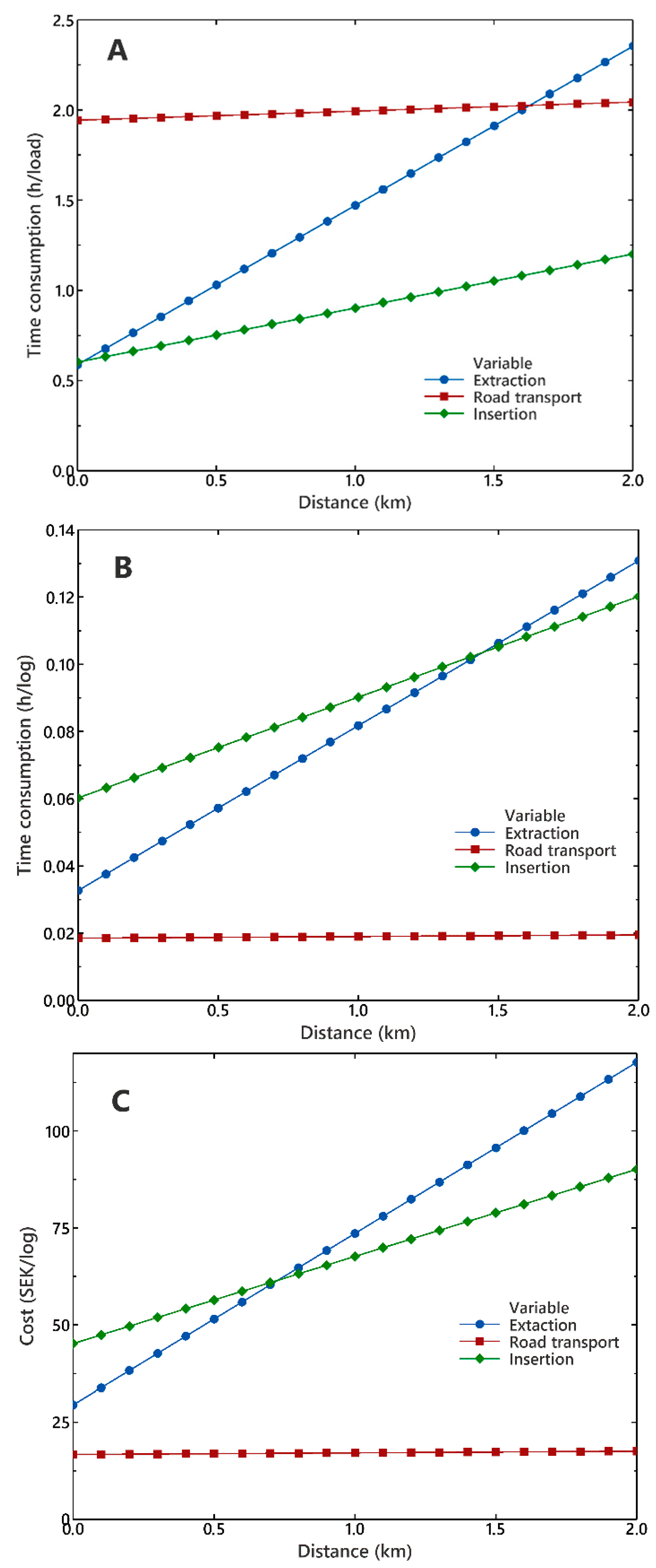
Due to the different nature of translocation work compared to normal forest operations, it is difficult to compare the observed time consumptions and costs to previous research. However, it can be noted that the driving speeds are in line with previous research on extraction [18,27] and road transport [28,29]. There is a lack of research about the forwarder used for the insertion (Terri ATD), but it can be noted that it was driven at a considerably higher speed than during extraction with conventional forwarders. Hence, the small load volume of the insertion forwarder is, to some extent, compensated by its higher speed. In relation to the forwarder used in the extraction, the insertion forwarder’s work becomes more competitive the longer the distances driven (Figure 3B,C).

In relation to costs, there is a limited amount of research to compare with. However, the cost of conventional logging can serve to put the costs in perspective. The average costs for harvesting trees and extracting the logs to roadside in Sweden are approximately 95 SEK/m³ for final felling, with average tree volumes of 0.23 m³ under bark and with 44% of the costs being attributable to the extraction [30]. So, assuming the insertion corresponds to two extraction costs, conventional harvesting, extraction and insertion would be 137 SEK per m³. Conventional Swedish road transport costs are approximately 86 SEK per m³ in Northern Sweden [30]. So, in total, conventional felling, extraction, road transport and insertion could be estimated to cost 223 SEK per m³. With a mean log volume of 0.24 m³ over bark as in this study, this corresponds to approximately 54 SEK/log, whereas it was observed to be almost seven times higher (363 SEK/log) for the corresponding work phases of actual translocation work (i.e., with the costs of the scientific evaluation excluded). There are substantial shortcomings in the comparison, but it, nevertheless, clearly highlights the considerably higher costs related to translocation of ecologically valuable, and sensitive, logs compared to fresh logs for industrial uses.

In this observational study, total time consumptions and costs were based on self-reported data from the contractors executing the translocation work. The self-reported data was also provided to the customer for reimbursement purposes, and thereby motivating correctness in relation to agreements and to maintain the business relationship. Thus, the self-reported costs were the actual costs invoiced for executing the studied work. The conducted time studies of some work phases gave input on how the invoiced costs would change under different conditions. Additional time studies could provide similar information for also the other work phases. To estimate the actual time requirements and the actual hourly costs (and not invoiced) would naturally also be of interest, but would require a larger study set-up and also data for estimating hourly costs of contractors.

Although the full cost of the project to expand the sand magazine is not known, the compensation costs can be expected to be relatively small in comparison. Compensation costs are, nevertheless, one of many costs in projects that often require large investments, so cost efficiency can contribute to at least two beneficial effects. The first is by making ecological restoration more likely to be used when costs can be kept low. The second is by providing increased benefits for a given cost, when the most cost-efficient measures can be chosen.

There are several possible ways to influence the costs, by choices related to the planning and execution of the operations, and by the qualitative requirements of the result of the operation.

The results showed that there is an increased cost with increased driving distances for all three work phases in which logs are transported (Figure 3B). The cost increase was substantial for both extraction and insertion. Hence, the closer to roads that the logs to be extracted can be collected, the lower the costs will be. Correspondingly, insertion costs will be lower the closer to the road the logs can be placed in the compensation area. In contrast, road transport contributed very little to overall cost and the cost increased very little with distance. Thus, an increase in road transport distance will have relatively little effect on overall cost, so translocation over larger distances is possible without substantial impact on overall cost. In fact, a doubling of the road distance driven would only have resulted in a 4% increase in costs per translocated log (0.40 SEK/km and log × 50 km/456 SEK/log). For future translocation projects, this knowledge should be beneficial in allowing the prioritization of short extraction and insertion distances over road transportation distances when trying to minimize costs.

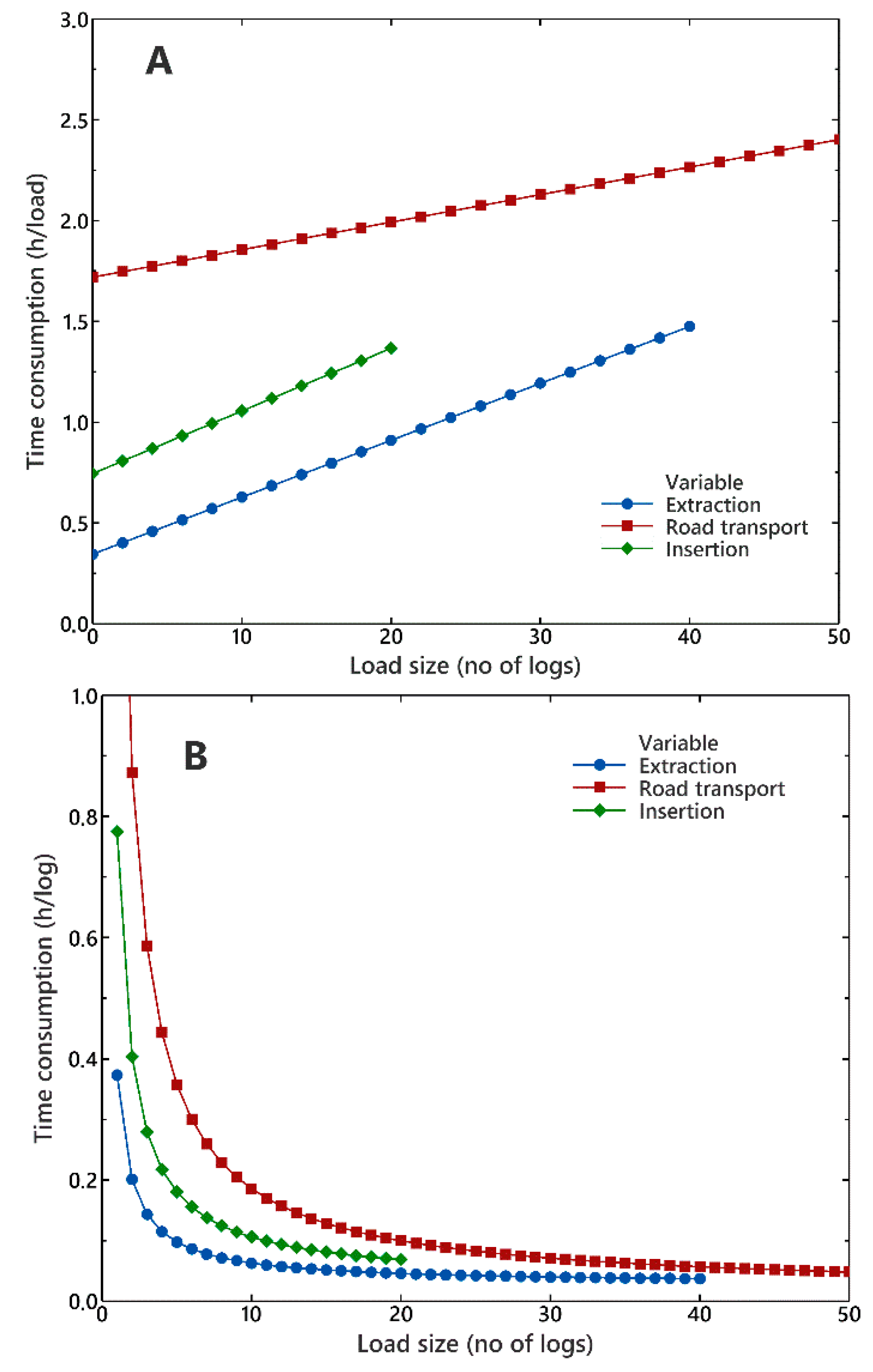
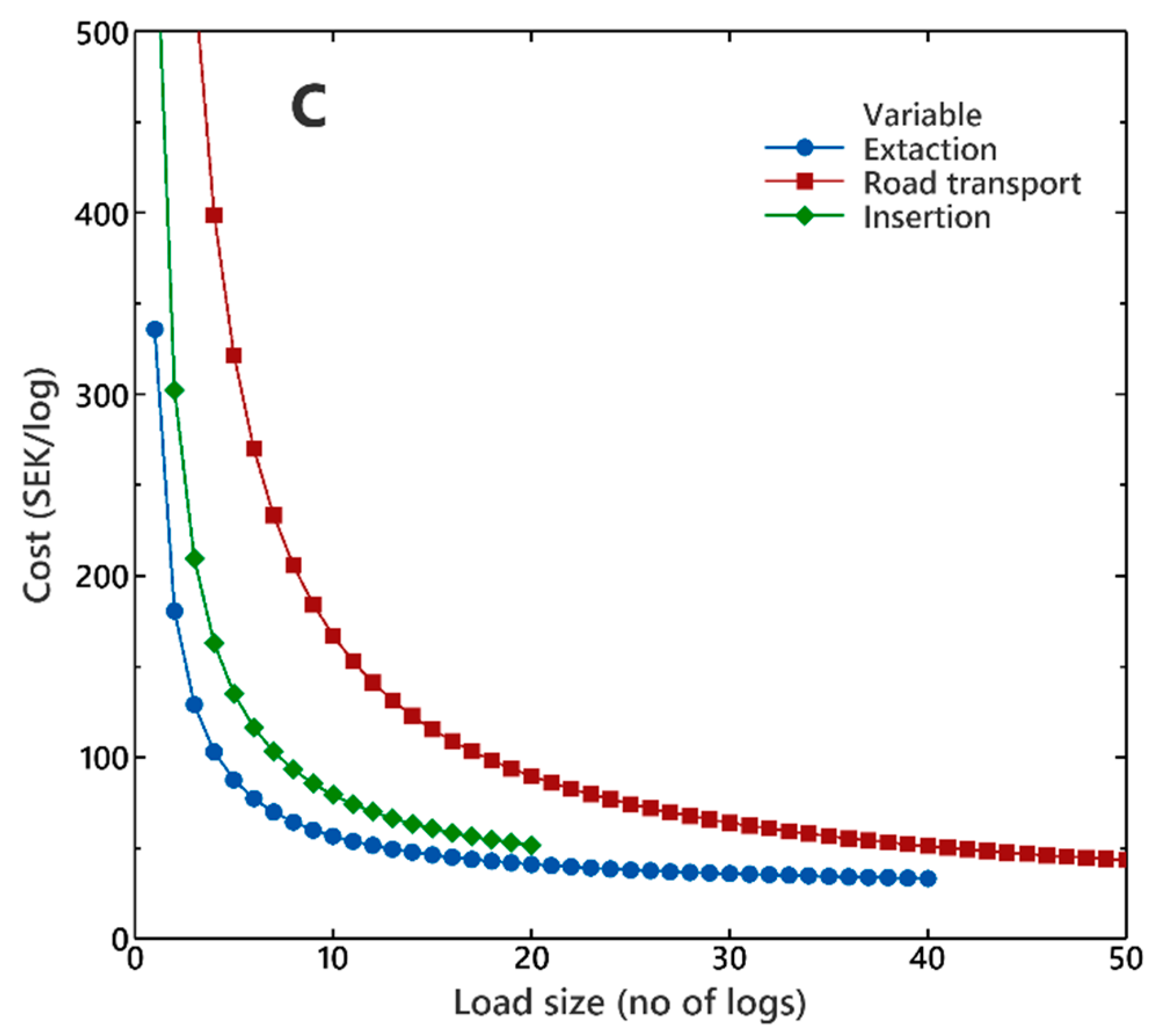
Another well-known time and cost driving factor that was not studied is the effect of log concentration. This can, briefly, be described as the more logs that are located in one place when being loaded or unloaded, the faster and thus cheaper the work [31]. Hence, if logs can be collected within a limited area during each round trip with the forwarder, the cheaper it will be. Similarly, it will be more efficient if the loading and unloading of trucks and the insertion forwarder can be carried out in concentrated areas. In fact, the organization of logs at the roadside landings was one important area of improvement highlighted by the operators in the study, in order to minimize the need for relocating the vehicles when loading/unloading different log types.

The operations described in this study were carried out for the first time by the people involved. It can be expected that repeating the operation will be quicker as these people gain more experience, and hence, the costs will decrease. A key way of improving extraction may be to use a different type of grapple than the conventional one used, preferably one that is small, straight and pointed to grip one log at a time without damaging the logs being loaded or the adjacent logs. Better planning and marking of log positions and log types, as well as clearer extraction trails, have been suggested by the operators to reduce the time for extraction, but it would also create extra work during extraction preparation. Furthermore, it would be desirable to only work with as many logs as are required for the relocation. In this study, 671 logs were produced during felling and subsequently extracted, but only 640 were road transported and inserted. The excess could be seen as a buffer to ensure that the desired number of logs of different qualities were available for the Road Transport and Insertion phases but, ideally, such an excess would not be necessary.

A rough estimation for the new improved planning and execution is that it could result in a total cost of 397 SEK/log, corresponding to a cost reduction of 15%. The estimation is the result of removing the time estimated to be associated with the 31 excess logs, a 30% decrease in time consumption during loading for both extraction and road transport (corresponding to better organization of roadside landings), and a subsequent 9% decrease in time consumption during extraction, road transport and insertion (corresponding to a general improvement in work efficiency due to experience).

The qualitative requirements of the operation greatly affected the cost. This was partly manifested by the high cost for the insertion, in part due to the choice of using a smaller forwarder to reduce the risk of damage to the ground in the compensation area. Thus, if ground damage had not been an issue, the use of a forwarder with a higher payload and thereby better cost-efficiency might have reduced costs. However, the quality of the translocated logs affected the cost even more, as indicated by the low load capacity utilizations (Table 5). If payload capacities were fully met, as with conventional logging, the costs would be substantially decreased. The challenge, however, is that the more decomposed and therefore fragile the logs are, the greater ecological value they might have as more rare- and threatened-species are associated with the late stages of decomposition [32,33]. Hence, there is a trade-off between costs and the qualitative properties of the translocated logs. Increasing payload usage by loading more logs with high ecological values carries with it an increased risk that log structures and species living on the logs would be severely damaged when piling them on top of each other. In fact, the most valuable logs in the impact area were not translocated since it was not considered feasible to move them due to their fragility [26]. Another way to utilize the payload capacity would be to translocate less ecologically valuable logs that can survive being transported in full loads. Yet another way would be to construct loads such that the most fragile logs were loaded on top with the most solid logs at the bottom of a load.

The level of decomposition of the logs could also be expected to influence the loading and unloading work. The more decomposed the logs are, the more carefully they need to be handled. The size of the logs is also a determining factor on the loading and unloading times. During road transport, the observed difference in mean loading times between the fastest log assortment (spruce logs, early decomposition) and the slowest (pine logs, intermediate decomposition) was 13.3 s per log. The same log categories were loaded fastest and slowest during insertion, with a mean difference of 23.4 s per log. It was not possible to evaluate whether the observed differences were statistically significant due to the aggregated data collection method, neither was it possible to evaluate possible reasons (such as differences in log sizes between classes).

When considering the choices related to qualitative results of the translocation, there is a trade-off between costs and time until a given ecological value is reached in the compensation area. If it is acceptable to wait for the ecological values to develop, economy of scale can be used in order to cut costs. Conversely, the time required to achieve high ecological values in the compensation area can be reduced by accepting higher costs.

To know the acceptable timeline for ecological values to develop, there is a need for knowledge about the speed at which such values develop under different treatments. The work carried out in this translocation project included facilitation of such scientific evaluation, which focused on evaluation of the effect of differences in concentration of dead wood. Hence, this study covered some of the costs of knowledge production and found that the operational work to carry out the scientific evaluation required an additional 75% of financial resources in addition to the resources needed for the actual compensation work. The operational work to lay out the experiment is only one part of an evaluation project. Thus, the costs related the researchers’ design of the experiment, the inventories required to follow up the results of the translocation, the data analysis and publication of results should be totaled to give the full cost of the scientific evaluation. A modest estimation is that those costs not accounted for in this study are of a magnitude 10–100 times higher than the observed cost related to carrying out the scientific evaluation.

To the best of our knowledge, this study is unusual in that it added a cost-efficient dimension to ecological compensation. The data from a single observational study should naturally be handled with care when being used in other contexts, and there is a need for additional studies to verify and refine the findings. However, the general results are in line with similar studies from conventional forest operations, indicating that similar cost-driving aspects are in action. Hence, the methodology seems applicable to operations within the field of ecological compensation, and could be applied to enable cost-benefit evaluations of possible alternatives. This would enable efficient use of scarce resources, both when it comes to the strict delivery of the compensation (i.e., to spend as few resources as possible on a decided compensation action) as well as to the ecological quality of different actions (i.e., to choose the action that gives a desired benefit-to-cost level).