Article

Quantifying Ecosystem Services of High Mountain Lakes across Different Socio-Ecological Contexts

1
Department of Ecology, University of Innsbruck, Sternwartestrasse 15, 6020 Innsbruck, Austria
2
Institute for Alpine Environment, Eurac Research, Viale Druso 1, 39100 Bolzano, BZ, Italy
3
Department for Limnology, University of Innsbruck, Mondseestrasse 9, 5310 Mondsee, Austria
*
Author to whom correspondence should be addressed.
Sustainability 2021, 13(11), 6051; https://doi.org/10.3390/su13116051
Submission received: 6 May 2021 / Revised: 26 May 2021 / Accepted: 26 May 2021 / Published: 27 May 2021

Abstract

:
Mountain lakes are highly sensitive to global change, requiring sustainable management strategies that support crucial ecosystem services (ES). However, small mountain lakes are rarely in the focus of ES assessments, and indicators are potentially lacking. Therefore, this study aimed at comprehensively assessing key ES of 15 study lakes located in two regions in the European Alps. We involved local stakeholders and experts to identify important ES. We quantified eight ES in non-monetary terms, using 29 indicators based on limnological, spatial and socio-economic data. Finally, we evaluated ES in relation to the socio-ecological context of the study lakes. The most important ES included surface water for non-drinking purposes, maintaining populations and habitats, outdoor recreation, aesthetic value, entertainment and representation, scientific research, education as well as existence, option, or bequest value. Quantitative results indicate varying levels of ES across the study lakes. Based on 12 different socio-ecological variables, we identified four groups of lakes differing also in five ES. Maintaining populations and habitats, aesthetic value as well as existence, option or bequest value were rather independent from the socio-ecological context. Our findings contribute to a deeper understanding of ES of mountain lakes, also supporting the development of sustainable management strategies in mountain regions.

1. Introduction

Freshwater lakes and ponds greatly contribute to human well-being by providing crucial ecosystem services (ES), such as water supply for domestic, agricultural, and industrial use, hydropower production, flood control, climate regulation, and outdoor recreation [1,2,3,4]. ES can be broadly defined as the contributions of ecosystems to human well-being [5,6,7]. Based on ecological functions and processes that represent the capacity of ecosystems to provide goods and services (natural capital), ES are generated by human interactions (human-derived capital) with nature to satisfy human needs [7,8,9,10]. Lake ecosystems, however, are highly susceptible to anthropogenic stressors [11,12,13]. Climate change, land-use intensification, water abstraction or water-level regulation, shoreline modification, and invasive species may lead to alterations of physical, chemical, and biological characteristics of lakes [12,14]. Since ES provision strongly depends on ecological functions and processes, such stressors may severely affect individual or multiple ES [13,15]. Despite the growing number of studies on ES of freshwater ecosystems, mostly focusing on large lowland lakes [3,16], knowledge on human–nature interactions related to small high mountain lakes is still scarce, but urgently required to develop sustainable management strategies in the light of global change [17].
High mountain lakes are considered particularly vulnerable to rising temperatures due to the amplification of global warming in high-elevated regions [11]. Higher temperatures reduce ice-cover duration and the volume of inflowing snow melt, which greatly affects hydrological patterns, as well as ecosystem processes, such as primary production due to increased lake water temperatures [18,19]. Moreover, high mountain lakes are more exposed to atmospheric nutrient inputs compared to those at low elevations with consequences on lake functions and species composition [11,12]. While such ecological changes influence ES provision, socio-economic changes alter the demand for ES. Since mountain regions are important water suppliers for downstream populations, the demand for water is expected to increase due to changes in precipitation patterns and population growth [20,21]. Increasing transformation of natural ecosystems in and outside mountain regions to intensively used land, a shifting socio-economic focus from agriculture towards tourism and changes in leisure behaviour increase the pressure on natural environments in mountain regions [22,23]. Spatio-temporal expansion of recreational activities may affect lake ecosystems as well as local socio-economic conditions in various ways. For example, the introduction of fish in naturally fishless lakes for recreational angling affects native amphibian species [24] as well as on nitrate concentrations due to fish feeding, resulting in eutrophication [19]. Moreover, hiking activities in proximity to lakes contribute to the growth of aquatic vegetation in high-mountain lakes, increasing the level of eutrophication [25]. Moreover, an increase in accessibility, which is often fostered to attract more tourists, may provoke conflicts among different recreational user groups or stakeholders [26].
In light of the above-mentioned changes and increasing pressures on ES and human society, a comprehensive assessment of ES is needed to support management and decision-making [27]. In the first step, relevant ES need to be identified and selected for further analysis. This is mostly performed based on data/model availability or literature reviews, but the involvement of local stakeholders allows for prioritizing context-specific ES [28]. Commonly, three categories of ES are distinguished, provisioning ES, regulating, and cultural ES [8,29,30]. ES have also been categorised, for example, in the Common International Classification of Ecosystem Services (CICES) [29] to improve consistency in ES assessments. The second step is the biophysical assessment of the selected ES. Many provisioning ES can be directly measured, but the quantification of regulating and cultural ES is more complex and needs different indicators or proxy data [5,9,31,32,33]. To quantify such indicators, different methods have been developed. These include biophysical methods that rely on direct or indirect measurements of data or ecological models [5,34,35]. Socio-cultural methods are mainly used to assess human preferences [32], while economic methods aim at assigning monetary values to ES. Finally, expert-based approaches based on lookup tables [9,36,37] are often applied if other data are lacking. Further steps may include the valuation of ES using monetary, qualitative, or socio-cultural metrics to raise awareness, compare ES across regions, implement payments for ES, among others [7]. Such valuation is not addressed in this study. Despite great advances in mapping and quantifying ES, the quantification of multiple ES of mountain lakes has rarely been in the focus of ES assessments and remains challenging due to their small spatial scale, which makes it difficult to obtain quantitative and spatially explicit data and to define indicators that can reveal differences in ES provision across different lakes [38].
In many ES assessments, people’s perceptions on the importance of ES are neglected, but this information is crucial for decision-making, as conservation measures are usually more effective if supported by local stakeholders [13]. This is of particular importance when it comes to trade-offs among multiple ES [39]. In addition, decision-making and management strategies are more effective if accounting for the specific socio-ecological context, which can influence people’s perceptions of ES [40]. For example, stakeholders valued recreational, cultural, and aesthetic ES in regions with high tourism intensity, while regulating ES were considered as more important in regions with recent impacts on productivity from pests [41]. Moreover, increasing tourism, land-use changes, and climate change can have huge impacts, for example, on the water availability in particular in water-scarce regions [42]. Decisions depend on future developments desired by the local communities [43], and a profound understanding of interactions between human and natural systems can support the achievement of sustainable management solutions [44].
This study aimed to address the above-mentioned knowledge gaps related to ES provided by small high mountain lakes by identifying and quantifying ES. Our specific objectives were:
  • Identifying the most important ES of small high mountain lakes;
  • Selecting suitable indicators for the biophysical quantification of the selected ES;
  • Evaluating ES in relationship to socio-ecological characteristics of the study lakes.
We addressed the first objective by involving local stakeholders and experts to prioritise ES in two study regions in the European Alps. After selecting multiple indicators for each selected ES, we quantified ES in non-monetary terms of 15 study lakes located in the two regions using mixed methods (objective 2). Finally, by grouping the lakes based on their socio-ecological context, we examined differences in ES provision between groups of lakes. Related findings aim to support the development of group-specific management strategies, which could be also applied in other regions with similar socio-ecological characteristics.

2. Materials and Methods
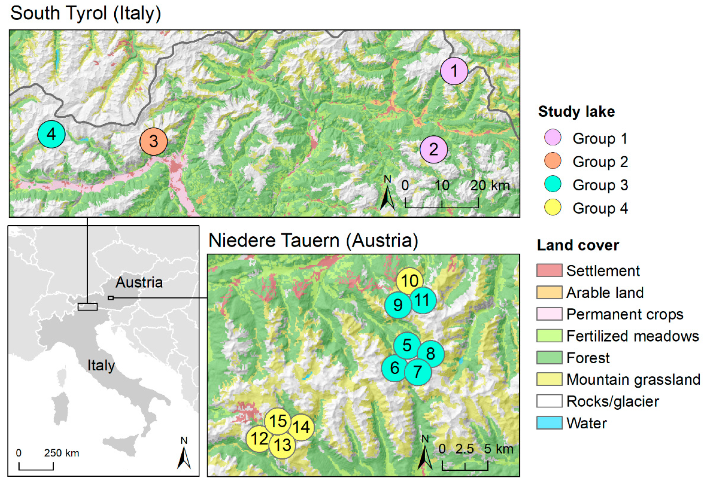
2.1. Study Sites

To account for local variability and distinct socio-ecological characteristics, we selected 15 small high mountain lakes located in two regions in the European Alps: (1) South Tyrol (Italy) with 4 lakes and (2) Niedere Tauern (Austria) comprising 11 lakes (Figure 1). Elevation of lakes varies from 1493 to 2758 m a.s.l. and lake size ranges between 0.54 and 43.24 ha (Table 1). Most lakes are located along the timber-treeline ecotone (alpine climatic zone) and bare rocks and meadows are the dominating land cover types in the catchment area, while trees (<6%) or shrubs (<24%) are less present [45]. Two lakes in South Tyrol (Antholzer See and Pragser Wildsee) are larger and located at lower altitude (montane climatic zone) and the catchment includes a higher share in forest (~30%). In general, the lakes become ice free during May/June and freeze during October/November [19]. Primary productivity in the water column is limited by the length of the vegetation period as well as the nutrient conditions. Water transparency is high and chlorophyll a concentrations indicating primary productivity are within the ultra-oligotrophic to oligo-mesotrophic range [46].
Due to their different geographic location in the southern and northern part of the main Alpine ridge, climate differs in the two study regions, being warmer and dryer in South Tyrol and cooler and wetter in Niedere Tauern [47]. Land cover composition in both regions is similar and comprises mainly forest, grassland and unused land, such as natural grassland, rocks, and glaciers, but Niedere Tauern has a higher share of forest, while South Tyrol comprises more agriculturally used land, with meadows and pastures at higher elevations and permanent cultures in the valley bottom [48]. South Tyrol has a mean population density of 72 inhabitants per km2 and about 33 million overnight stays yearly [49]. Niedere Tauern is less populated (24 inhabitants per km2 in the region of Liezen in Styria and 32 inhabitants per km2 in Upper Styria West) and tourism is less developed (Styria about 13 million overnight stays yearly) [50]. More specific, in proximity to the study lakes, i.e., within 30 min driving from the nearest access point to the lake, there are on average 15 overnights per inhabitant in Niedere Tauern during the summer season compared to 46 overnights per inhabitant in South Tyrol. The lakes are generally visited by hiking during the ice-free period and hiking times range from a few minutes to 5 h.

2.2. Identification of Key ES

To select ES that are considered as most relevant for the specific study region by local stakeholders and experts, we carried out a workshop in each region. First, stakeholders being familiar with mountain lakes were identified using a purposeful sampling approach [51] by analysing policy and media documents, interviewing local key informants and enlarging the group of relevant stakeholders through snowball sampling. During the workshop, participants were asked to indicate ES, which they associated with small natural mountain lakes. Since not all participants were familiar with the concept of ES, we used broader terminology referring to ES as “services, goods or contributions to human well-being” [40]. To foster a collaborative process and to reduce group-related bias, we relied on the established focus group and participatory methods for identifying ES [28]. Hence, participants first collected and discussed potential ES in small heterogeneous groups of four people. Each group then presented their results to all workshop participants on a flipchart. To identify key ES, we carried out a rating exercise where each participant could individually assign six points to the mentioned contributions. Subsequently, all participants discussed together the outcomes of the rating exercise. After carefully addressing diverging opinions, all participants agreed on priority contributions in an open plenary discussion. The entire workshop was moderated by two researchers to guide participants and to focus the discussion on the workshop objective without influencing participants’ opinions and choices. Finally, we aligned the workshop results to common ES terminology. After the workshop, two researchers attributed the key contributions of lakes that were identified by the participants based on collected key words as well as descriptions from the audio registration to ES classes defined in CICES [29]. Workshop participants were informed about the results after the workshop and asked for feedback, but they were not further involved into the selection of related ES indicators.
The workshop in South Tyrol was carried out in Bozen/Bolzano (Italy) in January 2020 with 12 stakeholders representing all relevant sectors, including nature conservation, water management, local authorities, tourism, economy, research and education, and NGOs. In Niedere Tauern, the workshop took place in Radstadt (Austria) in August 2020, involving 10 stakeholders from the sectors water management, economy, tourism, research and education, as well as NGOs.

2.3. Selection of ES Indicators

To quantify ES of small high mountain lakes that were prioritised by stakeholders (see Section 2.2), we first collected indicators from literature. As most studies focused on greater spatial scales or compared ES of different ecosystems, not allowing to identify variations in ES across different small mountain lakes, we also developed new indicators. Using a combination of indicators related to ecosystem conditions as well as potential and actual benefits can capture multiple facets of ES [9,31,52]. We therefore included multiple indicators (Table 2), describing various aspects of each ES at fine spatial scale enabling to detect differences between individual lakes. Moreover, indicators were selected considering the possibility for monitoring changes in ES over time, i.e., the impacts of global change on ES. We focused on the potential ES supply (stock of natural capital), which characterises the capacity of ecosystems to provide ES independently from their actual use (flows of benefits) [5,10]. The proposed indicators therefore mostly refer to the structure and function of the ecosystems, partly also accounting for human-derived capital or human preferences [53]. Indicators related to ‘entertainment and representation’ represent people’s interest in a specific lake and refer rather to the flow of benefits than to potential ES supply [5,10]. To assess the individual indicators in non-monetary terms, we used mixed methods, focusing on biophysical methods including direct measurements and modelling based on primary data (e.g., limnological and climate data) and socio-cultural methods (e.g., preference surveys). In the following, we provide details on each ES and related indicators.

2.3.1. Surface Water for Non-Drinking Purposes (Water)

This ES refers to surface water that can be used for non-drinking purposes such as industry, irrigation or energy production [29]. To quantify the contribution of each lake, we used two indicators describing the potential supply, as data on water abstraction were not available. The storage capacity refers to the amount of water that can be stored by the lake, i.e., the lake volume. Water availability corresponds to the amount of water that is available within the lake watershed derived from the water balance during the summer period (May–August) accounting for seepage, surface runoff and interception [55,56].

2.3.2. Maintaining Populations and Habitats (Habitat)

This ES focuses on the maintenance of nursery populations and provision of suitable habitats (food, protection) for plant and animal species to sustain lifecycle and to protect habitats and gene pools [29]. We selected three indicators that describe characteristics of the littoral lake zone, as complex littoral areas provide important habitat and shelter for different species, e.g., as nursery and spawning areas or suitable structures for aquatic invertebrates [60,61,62,63]. Littoral substrate complexity was calculated based on the mapping of three major substrate classes (silt/clay/muck, gravel, and boulder/bedrock), which were ranked by size (silt to bedrock). We then calculated mean values weighted with the percentage coverage. Shoreline development was calculated as the ratio of the length of the shoreline to the length of the circumference of a circle of area equal to that of the lake [64]. Riparian vegetation complexity included vegetation coverage of shore habitat types as well as land cover types along the lake (~up to 20 m). We used four cover classes (absent (0), sparse (0–10%), moderate (10–40%), heavy (40–70%, and very heavy (>70%) [65]). To each cover class, we assigned the respective arithmetic midpoint values (0%, 5%, 25%, 57.5%, and 87.5%) and calculated mean values weighted by percentage coverage of each type along the shoreline. Both indices were standardised and then aggregated into a single index.
High water quality supports ecosystem health and functioning [13,39]. Therefore, the trophic state of the lake water was described using the three variables chlorophyll-a, the concentration of total phosphorus and Secchi depth [46,66]. Each variable was assigned to a trophic state based on class ranges (Table A1). Subsequently, the three variables were combined into a single index (1 = eutrophic, 2 = mesotrophic, 3 = oligo-mesotrophic, 4 = oligotrophic, 5 = ultra-oligotrophic). Moreover, nitrate expressed by the concentration of reactive nitrogen was included as an indicator for water quality [67].
To describe the habitat for plant species, including vascular plants and mosses, we derived the total number of different species from regional databases [57]. Red list species were weighted double.

2.3.3. Outdoor Recreation (Recreation)

Outdoor recreation was defined as physical interactions with the natural environment (abiotic and biotic) [29], including recreational activities that can be carried out at lakes, such as swimming, bathing, recreational fishing, boating, hiking, and birdwatching. Due to the remoteness and low water temperatures of mountain lakes, we focused on indicators describing different aspects related to accessibility and recreational opportunities, indicating the potential supply.
Accessibility is crucial to reach mountain lakes and steep terrain or long distances may prevent people to reach the lake [26]. We identified access difficulty of the main hiking trail for reaching the lake according to the scale of the Swiss Alpine Club (T1 (easy)–T6 (very difficult). The access level instead describes the type of recreational activities and was determined based in qualitative assessment and expert knowledge, distinguishing three classes [68]: (1) primary contact (i.e., immersive aquatic activities, such as swimming or kayaking); (2) secondary contact (i.e., activities that can be carried out at the lake without direct contact to the water such as fishing or boating); (3) visual contact only (i.e., activities that are carried out at the lake shore or in proximity to the lake such as hiking or cycling). Warm or hot days support more water-related activities than cold weather [69]. The number of warm days (≥20°C) per year was derived from local climate stations. If no station was located in proximity to the lake, data from the nearest station was used after correcting the measured temperatures with elevation (−0.6 °C per 100 m increase in elevation). In mountain areas, hiking is one of the most appreciated recreational activities in the summer [70]. We therefore calculated the length of hiking trails (hiking at lake) around the lake (distance from lakeshore ≤ 50 m) in relation to the lake perimeter to evaluate the opportunities for walking or hiking close to the lake. Human-made infrastructures and facilities are important for providing or improving recreational opportunities [9,71]. The number of tourist facilities (picnic area, benches, playground, etc.) was standardised in relation to the length of the shoreline.

2.3.4. Aesthetic Value (Aesthetic)

The aesthetic value is related to the characteristics of the natural environment (abiotic and biotic) that enable aesthetic experiences in direct interaction with nature [29]. Here, we focused on the visual characteristics of the lake and the surrounding landscape. Water clarity is important for aesthetic appreciation, often associated with water quality, and was measured by Secchi depth [72,73,74]. Littoral preference was calculated based on the mapping of littoral habitat types, to which we assigned preference scores obtained from a photo-based questionnaire [58] weighted by the length of each habitat type. Similarly, land cover preference included land cover types near the lake (~ up to 50 m), to which we assigned preference scores from the photo-based questionnaire [58] weighted by the length of each land cover type. Landscape beauty comprises the landscape within 500 m buffer around the lake and was derived through a spatially explicit modelling approach [75]. Viewpoints were randomly distributed (ca. 70 points km−2) in the 500 m buffer zone. For each viewpoint, a 360° viewshed was calculated based on a digital surface model (DSM) to identify the visible area up to 1500 m. After overlaying the visible area with a land cover map, 11 landscape metrics were calculated and related to people’s preferences from surveys via a regression model, estimating aesthetic landscape preferences. To viewpoints without a vista, i.e., located within forest, the preference score from the survey was assigned. Finally, we calculated mean preference scores of all viewpoints located in the buffer area for each lake. For further details on the methodology, see [75].

2.3.5. Entertainment and Representation (Representation)

Natural characteristics can be used for entertainment or representation, e.g., films, tourism brochures [29]. We used three indicators (Google Videos, Google Trends, and Instagram) measuring the people’s interest in the specific lake [76,77]. We determined the number of videos, the search interest relative to the benchmark term ‘mountain lake’, and the number of posts by searching for German or Italian lake names in the different databases.

2.3.6. Scientific Research (Research)

This ES is generally understood as characteristics of the natural environment (abiotic and biotic) that support scientific research [29]. Here, we focused on the relevance of mountain lakes for research on climate change impacts [11,13,18,19]. High mountain lakes are considered highly suitable as field sites or model systems to detect environmental changes due to their remoteness and extreme environmental conditions [14]. Such lakes are less affected by direct impacts from human use, while they are more exposed to atmospheric inputs than lowland lakes [11,13,19]. Important criteria for supporting such research activities include a high degree of naturalness and the absence of human use such as livestock farming and intensive tourism, which increase nutrient inputs and affects the ecological state of lakes [12,13,19,25,78]. As our study lakes are mostly used for recreational purposes, we used two indicators related to remoteness in terms of accessibility, as longer walking time and higher path difficulty can prevent people to reach the lake [26] and, thus, limit impacts from recreational use [25,78]. Access time refers to the walking time of the ascent to the lake from the nearest access point (parking, cable car, etc.). For access difficulty, see Section 2.3.3. Moreover, livestock farming in the lake watershed can alter water quality through increased nutrient inputs [79,80]. Since data on livestock units were not available, we used the percentage coverage of land cover types within the watershed that can be used for grazing, i.e., natural grassland and heathland, as proxy for potential presence of livestock farming.

2.3.7. Educational Value (Education)

Characteristics of the natural environment (abiotic and biotic) enable educational activities [29]. We included indicators that assess the lake’s suitability for educational activities at the lake by assessing the potential presence of visible/observable species [81], indicated by littoral structure complexity (see Section 2.3.2). To benefit from educational values of mountain lakes, we considered the access time (see Section 2.3.6), as closer lakes can be visited also by school classes or people that are not used to long hikes. Moreover, we included the number of potential beneficiaries in proximity to the lake, representing the level of interest in environmental education. Beneficiaries included residents and tourists (number of overnights), who can reach the nearest access point to the lake (parking, cable car, etc.) within 30 min driving by car. The number of overnights were first converted into a ‘permanent resident equivalent’ by dividing the total number of nights by 365 [82], and then added to the number of residents to indicate the total number of beneficiaries.

2.3.8. Existence, Option, or Bequest Value (Existence)

To measure existence, option or bequest value [29] related to mountain lakes, we used three indicators related to different aspects. As the designation of a location as protected area recognises the conservation value of ecosystems [83], we used protected area and identified the IUCN category to indicate the level of protection. Uniqueness and rareness are also important criteria for conservation, as the loss of specific habitats or sites could diminish the number of known species [83]. We therefore measured lake abundance by identifying the number of lakes with an area greater than 0.1 ha and up to a distance of 5 km from the study lake. Moreover, ecosystem integrity, referring to the natural state of ecosystems and processes, may be expressed by the level of anthropogenic influence [84]. To indicate the agricultural intensity linked to livestock farming, we used the percentage coverage of land cover types within the watershed that can be used for grazing, since livestock farming for our study lakes are the most important human activities [79,80].

2.3.9. Total ES Index

To obtain a total ES index in non-monetary terms that is comparable across study lakes, we first rescaled all individual indicators to values between 0 and 1 (min–max normalisation), as indicators had different units. We then calculated a mean index for each ES based on the related indicators. In this way, all indicators attributed to a specific ES were given the same weight, with individual ES indices ranging between 0 and 1. Finally, a total ES index was calculated by summing all eight ES. ES were not weighted based on their prioritisation in the different regions due to lacking information on their relative importance. The total ES index has a potential maximum of eight and can be used to compare different lakes in terms of ES provision.

2.4. Evaluation of ES within the Local Socio-Ecological Context

To examine whether differences in ES occur in different study lakes, we collected various socio-ecological context variables (Table 3). These variables describe lake characteristics, environmental conditions, land cover, accessibility and beneficiaries. Variable values were derived by own calculations overlaying different spatial datasets using ArcGIS (version 10.4, ESRI, Redlands, CA, USA).
We applied cluster analysis to derive groups of lakes with similar socio-ecological characteristics. First, we tested correlations among all variables applying Pearson correlation and excluded those that highly correlated (Table 3). Based on 12 remaining variables, we applied hierarchical cluster analysis in SPSS Statistics (version 26, IBM, Armonk, NY, USA) using the squared Euclidean distance to measure the dissimilarity of the variables and applying Ward’s linkage method to aggregate the clusters. Based on the agglomeration coefficient, measuring heterogeneity as the distance at which clusters are formed, we decided to use the four-cluster solution. To examine whether differences in ES of the study lakes in one of the four groups can be explained by socio-ecological differences, we applied one-way ANOVA based on the standardised ES indices (see previous section).

3. Results

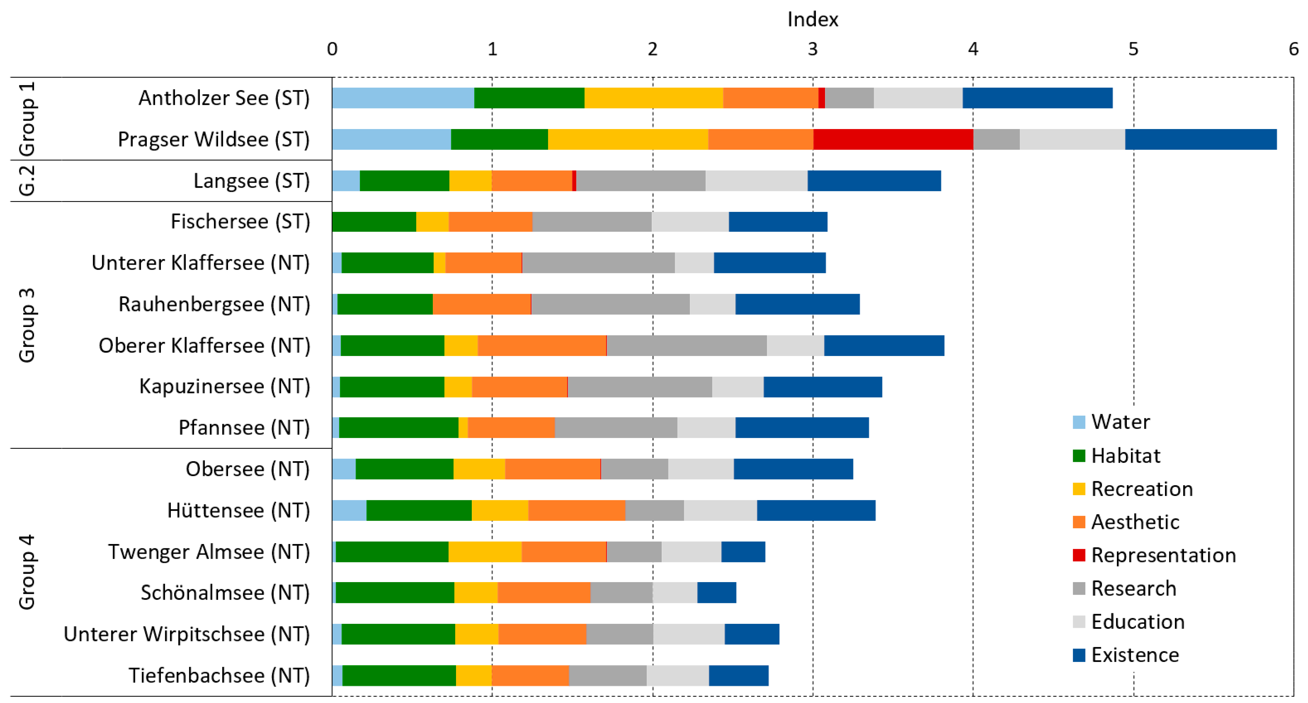
3.1. Key ES of High Mountain Lakes

Stakeholders prioritised eight different ES across both study regions, of which six were cultural ES (Table A2). In both study regions, three equal ES were selected by stakeholders, namely habitat, as well as recreation and aesthetic. While stakeholders in South Tyrol additionally indicated water and entertainment as important, stakeholders in Niedere Tauern named research, education, and existence.
We quantified all eight ES in non-monetary terms in both study regions using various indicators (Table 2). Mean ES indices varied across the 15 study lakes (Figure 2 and Table A3). Compared to the higher elevated lakes, the two larger and lower elevated lakes in South Tyrol had generally higher ES indices, in particular, for water, recreation, and representation. Lakes generally differed also in research, education, and existence, while less differences occurred for habitat and aesthetic.

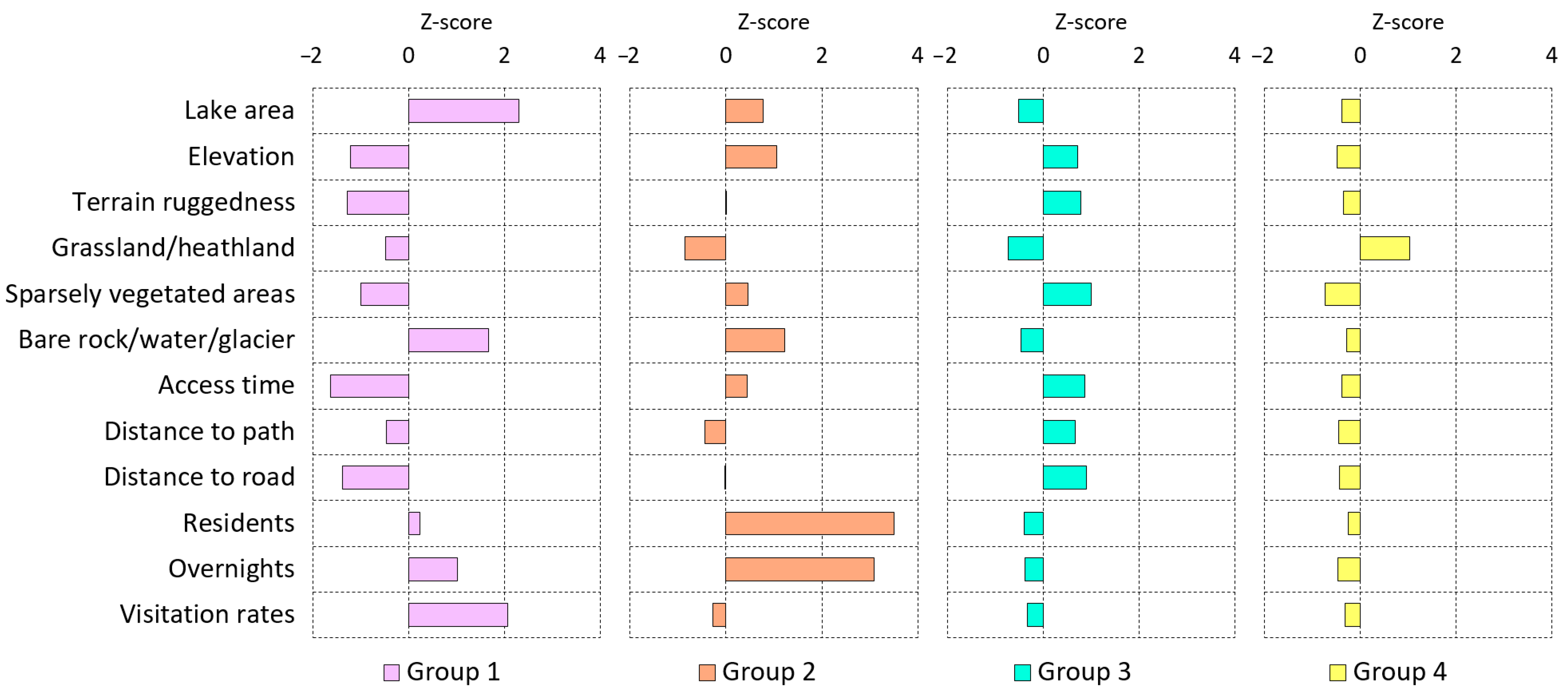
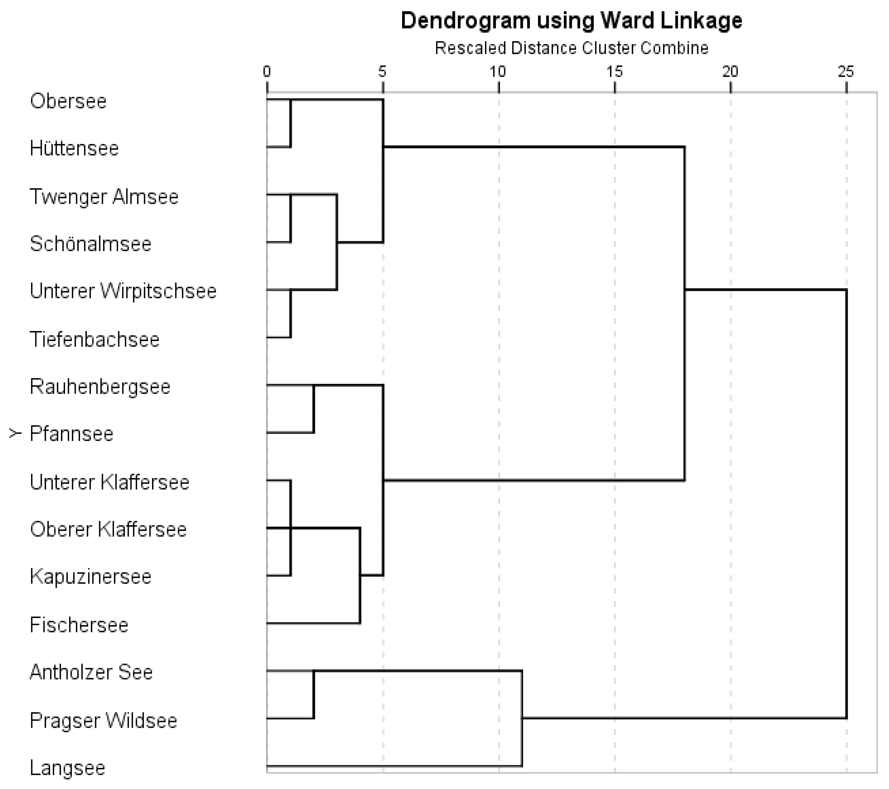
3.2. Socio-Ecological Differences

The lakes were grouped based on 12 socio-ecological context variables by hierarchical cluster analysis into four groups (see also Figure 1 and Figure A1), differing in socio-ecological characteristics (Figure 3 and Table A4):
  • Group 1 (Antholzer See and Pragser Wildsee) is characterised by large lake size, low elevation, good accessibility, a high number of beneficiaries (in particular, tourists) and high visitation rates.
  • Group 2 (Langsee) is located at high elevation in a landscape with predominantly bare rocks. Although it has a very high number of beneficiaries (in particular, residents), visitation rates are lower than for Group 1 due to a high access time.
  • Group 3 (Fischersee, Unterer Klaffersee, Rauhenbergsee, Oberer Klaffersee, Kapuzinersee, Pfannsee) comprises small, high-elevated, and remote lakes that are difficult to reach. Compared to Groups 1 and 2, this group has less beneficiaries and lower visitation rates.
  • Group 4 (Obersee, Hüttensee, Twenger Almsee, Schönalmsee, Unterer Wirpitschsee, Tiefenbachsee) includes lakes that are on average lower elevated and easier accessible than Groups 2 and 3, but the number of beneficiaries and visitation rates are similar to Group 3.
Most ES indices (water, recreation, representation, research, and education) differed significantly across the four groups (Table 4). In contrast, habitat, aesthetic, and existence were not strongly related to the socio-ecological context. Above-average indices occurred mainly for Group 1 and 2, while Group 3 and 4 had mostly below-average indices (Figure 2). In specific, Group 1 had greatest above-average indices for all ES with the exception of research. Group 2 had above-average indices for research and education. While research was also above-average for Group 3, recreation was below average. Group 4 had below-average indices for all ES, in particular research.

4. Discussion

In comparison to large lowland lakes, which are highly important for provisioning or regulating services [3,4,17], our results indicate that key ES of natural high mountain lakes include mostly cultural ES, which is probably due to several factors. One reason may be the small size of most natural lakes, which makes them less suitable for water provision, energy production or fish production compared to large lakes [3,86]. Another reason is their remoteness and often limited accessibility, contributing to maintain high level of naturalness of the lake ecosystem as well as the surrounding landscape. Accordingly, natural mountain environments were found being highly appreciated for various cultural ES in previous studies [75,87,88,89]. Several lakes are recognised as natural monuments in South Tyrol [90] and 14 of the study lakes are located in protected areas (e.g., natural parks, Natura 2000, UNCESCO biosphere reserves), which underlines their high importance for biodiversity conservation [83] and cultural ES [88]. Consequently, such lakes are better protected from intensive human use or the construction of new infrastructure through regulations, e.g., [91], assuring the sustainable use of natural resources.
Stakeholders in both study regions agreed on several ES, which can be considered as generally relevant for high mountain lakes in the European Alps, as confirmed by other studies [75,92,93]. Differences in identified ES between the two study regions can be explained by differences in the socio-ecologic context influencing the stakeholders’ perceptions. In South Tyrol, water scarcity is an issue [55] and the runoff from Langsee is already used for irrigation, whereas land-use and climate are different in Niedere Tauern with less pressure on water resources. The selection of representation in South Tyrol can be mainly related to the Pragser Wildsee, which has become famous by the Italian television series ‘Un passo dal cielo’ (One Step from Heaven) and which is highly disseminated by social media such as Instagram [94] or Flickr [92]. Although existence and education were also discussed in context with other ES, such as habitat and aesthetic in South Tyrol, it was not prioritised but considered as own ES in Niedere Tauern.
The selection of specific ES in each study region by the stakeholders was also broadly reflected and refined the ES indices of the four groups by accounting for the size and location of the lake (e.g., climate, accessibility), tourism development (e.g., infrastructure, touristic facilities), as well as socio-economic variables (e.g., potential beneficiaries, visitation rates). Such differentiation is very important with regard to decision-making, suggesting that lakes belonging to different types of groups require different management strategies. For Group 1, including lakes that are easily accessible and have elevated levels of beneficiaries and visitation rates, a focus needs to be set on visitor guidance, awareness raising, and regulating accessibility due to increasing pressure on the environment [25,95,96,97]. In the case of the Pragser Wildsee, local authorities have already taken measures to restrict the accessibility by car for limiting the number of visitors in order to reduce negative effects on the environment and the socio-economic context [98]. Despite high numbers of potential visitors in proximity to the lake, the lake of Group 2 is less visited due to its remoteness, but tourism management is still more important compared to lakes belonging to Group 4 with similar levels of accessibility but lower pressure from recreational use. Lakes of Group 3, which have intermediate levels of accessibility, seem not yet subject to high pressure, but this depends on future tourism development in the greater region or uncontrollable dynamics of social media that can cause overtourism [94].
Further issues may require the attention of policymaking, but are not reflected by the groups; for example, issues related to uses such as fishing or livestock farming, which can lead to great alterations of the lake ecosystem [13,19]. In addition, the legal framework may be important for governance of ES of mountain lakes in our study regions and can be a source for potential conflicts [26]. While lakes in South Tyrol are public goods and public institutions are responsible for the lake management, mountain lakes in Niedere Tauern may be private property and lake owners can prevent the access and use of the lake. Moreover, lake owners are currently not obliged to implement specific management measures or participate at monitoring programs, as lakes that are smaller than 0.5 km2 are not included in the Water Framework Directive of the European Union [99].
Another issue of increasing urgency is that climate-induced changes may severely threat ES provision in the future. For example, regional differences in precipitation pattern may further increase water scarcity in the southern part of the Alps [20,42] and lead to changes in ES, as well as to shifting priorities in the use of mountain lakes, i.e., water provision may become more important than other types of uses. Other ES, such as habitat or aesthetic, may be affected by increasing level of eutrophication originating from higher lake water temperature, atmospheric nutrients inputs, and anthropogenic use, which reduces water clarity and alters water quality [13,18,19,74]. Future research focusing on relationships between ecological processes and ES provision, as well as scenario analysis, may provide deeper insights supported by quantitative data and reveal changes over time.
In this study, we set high effort in identifying and calculating suitable indicators for evaluating the eight key ES, which allow detecting differences among small lakes and monitoring changes in ES over time. We used mixed methods (i.e., ranging from biophysical to socio-cultural methods) to assess multiple indicators of each ES. In this way, the multifaceted characteristics of ES could be captured in a more holistic way [31,52]. Due to data restrictions, it was not possible for all ES to combine ecological indicators with socio-cultural indicators. Results could be improved, for example, for water by including the amount of water abstractions [34] or the area of irrigated land [100]. Further indicators could also be useful, for example, related to fish and amphibian species, which could be relevant for ES such as habitat or education [81]. Moreover, our results mostly reflect the potential ES supply without quantifying the demand for ES. Such information, however, is useful for decision-making, as it can reveal, for example, supply-demand mismatches and incongruities with sustainable development [101]. Finally, we weighted all ES equally across the study regions due to lacking information on the relative importance of ES, although ES prioritisation differed in South Tyrol from Niedere Tauern for some ES, suggesting that, for example, water and representation are more important in South Tyrol, while research and education have greater weight in Niedere Tauern. However, differences in importance of individual ES within the same regions or across groups of lakes remain unclear and future research should collect such information. This is especially important in the light of expected climate change impacts [11,13], which can also shift priorities and the demand for ES depending on the socio-ecological context [41,42].
In terms of transferability, the findings of this study can be useful to researchers and practitioners in other mountain regions. First, as high mountain lakes worldwide are characterised by similar environmental conditions [11,13], a better understanding and characterization of ES was achieved in this study that may also apply to other small mountain lakes. Second, the proposed indicators can be applied to other lakes, given the availability of data, and are not limited to high mountain lakes. Nevertheless, it may be necessary to adapt some indicators that were based on specific survey results (e.g., preferences for littoral habitat types or adjacent land cover types). Finally, by grouping the lakes based on their socio-ecological characteristics, our findings can be useful to define and implement group-specific management strategies without the necessity to quantify all ES.

5. Conclusions

This study contributes to research and decision-making in several ways. We advance knowledge on ES by identifying eight key ES of mountain lakes involving local stakeholders. We also propose a comprehensive set of indicators for their quantitative assessment in non-monetary terms. By placing the lakes in the local socio-ecological context, our findings contribute to a deeper understanding of the underlying mechanisms for ES provision, as ES, such as water, representation, research, and education generally differed across groups of lakes. However, our results also suggest that habitat, aesthetic, and existence are important ES provided by all lakes, independently from the socio-ecological context. Socio-ecological differences seem to have also influenced stakeholders’ perceptions, and hence, the prioritization of specific ES, greatly matching differences in ES across groups of lakes.
Our findings provide valuable insights for decision-making and for developing sustainable management strategies, which can be tailored to the specific local context, accounting for environmental conditions and socio-economic requirements and values. Hence, management strategies should be defined based on natural characteristics of the lake, the level of accessibility, and tourism development and intensity, which differ across the four identified groups. To manage future impacts of global change on ES of mountain lakes, further research should deepen the understanding of ecological processes in relation to ES provision, as well as widen the focus on human–nature interactions by accounting for trends in ES demand.

Author Contributions

Conceptualization, U.S.; methodology, U.S., M.E., H.P., V.F. and R.K.; formal analysis, U.S.; data curation, U.S., M.E., H.P., V.F. and R.K.; writing—original draft preparation, U.S.; writing—review and editing, M.E., H.P., V.F. and R.K. All authors have read and agreed to the published version of the manuscript.

Funding

This research was carried out within the project CLAIMES (Climate response of alpine lakes: resistance variability and management consequences for ecosystem services) under the Earth System Sciences research programme, which is an initiative of the Austrian Academy of Sciences financed by the Austrian Federal Ministry of Education, Science and Research.

Institutional Review Board Statement

Not applicable.

Informed Consent Statement

Not applicable.

Data Availability Statement

The data presented in this study are available in the Appendix A.

Acknowledgments

We thank Gry Larsen, Josef Franzoi and Roland Psenner of the Department of Limnology of the University of Innsbruck (Austria) for carrying out chemical analyses. We also thank the Institute of Alpine Environment of Eurac Research (Bozen, Italy) for providing limnological data of the study lakes, which were measured in the project CHANGELAKE by Karin Koinig. Orthophotos and digital elevation models were provided by Land Salzburg © SAGIS and Geodaten GIS-Steiermark.

Conflicts of Interest

The authors declare no conflict of interest.

Appendix A

Table A1. Value ranges of three parameters (total phosphorus, chlorophyll a, and Secchi depth) used to identify the trophic class of lakes [46,66].
ParameterUltra-OligotrophicOligotrophicMesotrophicEutrophic
Total phosphorus [µg/L]<4.854.85–13.314.5–49.038.0–189.0
Chlorophyll a [µg/L]<0.80.8–3.43.0–7.46.7–31.0
Secchi depth [m]>105.3–16.52.4–7.41.5–4.0
Table A2. Prioritised ES in the two study regions.
ESSouth TyrolNiedere Tauern
Waterx
Habitatxx
Recreationxx
Aestheticxx
Representationx
Research x
Education x
Existence x
Figure A1. Dendrogram of the cluster analysis for grouping the study lakes based on their socio-ecological context.
Sustainability 13 06051 g0a1
Table A3. Indicator values of the 15 study lakes. All indicators were subsequently standardised and aggregated to quantify each ES.
ESIndicatorUnitAntholzer See—Lago di AnterselvaPragser Wildsee—Lago di BraiesLangsee—Lago LungoFischersee (Saldurseen)Unterer KlafferseeRauhenbergseeOberer KlafferseeKapuzinerseePfannseeOberseeHüttenseeTwenger AlmseeSchönalmseeUnterer WirpitschseeTiefenbachsee
WATERStorage capacity106 m311.045.302.580.030.50.20.60.10.00.80.20.40.20.10.1
Water availability106 m3 y−1845310,8881182138364636279579722429452811827311421228
HABITATLittoral substrate complexityindex0.400.660.560.790.590.730.970.630.580.480.490.360.410.520.42
Shoreline developmentindex2.112.763.222.312.122.422.442.263.332.532.442.012.332.002.47
Riparian vegetation complexityindex0.890.700.450.130.360.110.000.280.330.680.810.650.700.700.75
Trophic stateindex4.004.003.003.00nd4.004.005.005.004.004.004.004.005.004.00
Nitrate NO3-N mg l−10.220.300.130.060.110.130.090.110.080.230.200.000.000.110.08
Plant species n13.07.02.01.0ndndndndndndndndndndnd
RECREATIONAccess difficulty index003344443112222
Access level index112233223222222
Warm days days y−156.5058.7114.650.9021.100.240.100.571.626.249.430.710.715.623.19
Hiking at lake m0.711.230.250.300.000.000.360.430.000.310.420.590.120.290.06
Tourist facilities n km−12.893.630.350.000.000.000.890.000.000.000.002.870.940.000.00
AESTHETICWater clarity m7.67.66.44.5nd8.88.210.87.48.26.08.58.86.04.5
Littoral preference index0.100.180.200.330.130.170.620.110.120.170.190.120.120.150.15
Land cover preference index0.400.450.100.180.130.200.200.150.150.220.350.100.170.260.21
Landscape beauty index7.537.5410.458.8811.0811.0712.0210.5011.5310.529.1311.1011.049.789.61
REPRESENTATIONVideos n860102,000120012188188188188184561131244220931
Google Trends n0.162.050.120.02ndndndndndndndndndndnd
Instagram n16,224426,8292272230904904904904232953004254821125
RESEARCHAccess time min552101503003003152402101309013521090110
Access difficulty index003344443112222
Livestock farming %9.5214.050.000.008.220.000.006.2011.5037.6941.5985.3595.6150.7237.07
EDUCATIONLittoral structure complexity index0.400.660.560.790.590.730.970.630.580.480.490.360.410.520.42
Access time min552101503003003152402101309013521090110
Beneficiaries n63,27471,847257,25225,49616,78616,78616,78616,78634,76134,76134,76141,06018,97118,97118,971
EXISTENCEProtected area category222022222221111
Lake abundancen8521103127292817171630303537
Agricultural intensity %9.5214.050.000.008.220.000.006.2011.5037.6941.5985.3595.6150.7237.07
Table A4. Values of socio-ecological context variables of the 15 study lakes.
TypeVariableUnitAntholzer See—Lago di AnterselvaPragser Wildsee—Lago di BraiesLangsee—Lago LungoFischersee (Saldurseen)Unterer KlafferseeRauhenbergseeOberer KlafferseeKapuzinerseePfannseeOberseeHüttenseeTwenger AlmseeSchönalmseeUnterer WirpitschseeTiefenbachsee
LakeLake area103 m2432.42358.23195.895.3538.3627.6053.2322.7314.4672.5146.6929.9152.4727.4134.66
Lake perimeterm2771330928463388318041127682800136010556961068662918
Watershed area103 m218,87129,30619943180144460592212153020567213230612811378
EnvironmentElevationm a.s.l.164214932381275821032264231021461968167315022118211217011844
Terrain ruggednessindex576598713955734788728827708749743663678609624
Precipitationmm y−19558591113128515501543153515441554154115241472147214661466
Land coverForest/shrub%28.9632.880.000.000.000.000.000.000.000.000.000.000.000.400.00
Grasslands/heathland%10.3414.050.000.008.220.000.006.2011.5037.7944.9985.3595.6162.0837.07
Sparsely vegetated areas%24.2524.5773.3996.9791.78100.00100.0093.8066.9140.3138.7314.654.3937.5262.93
Bare rocks/glaciers/water%36.4528.5026.613.030.000.000.000.0021.5821.9016.280.000.000.000.00
AccessibilityAccess timemin552101503003003152402101309013521090110
Distance to pathm00422154511912298322540
Distance to roadm3046424811499381147971885993237145710262811399149123832268
BeneficiariesResidentsn48,71354,533221,54220,31914,88014,88014,88014,88032,33032,33032,33038,29018,36318,36318,363
Overnights103 n y−1262131176428932343343343343438438438499109109109
Visitation ratesn873487131211162222

References

  1. Allan, J.D.; Manning, N.F.; Smith, S.D.; Dickinson, C.E.; Joseph, C.A.; Pearsall, D.R. Ecosystem services of Lake Erie: Spatial distribution and concordance of multiple services. J. Great Lakes Res. 2017, 43, 678–688. [Google Scholar] [CrossRef]
  2. Fu, B.; Xu, P.; Wang, Y.; Yan, K.; Chaudhary, S. Assessment of the ecosystem services provided by ponds in hilly areas. Sci. Total Environ. 2018, 642, 979–987. [Google Scholar] [CrossRef] [PubMed]
  3. Sterner, R.W.; Keeler, B.; Polasky, S.; Poudel, R.; Rhude, K.; Rogers, M. Ecosystem services of Earth’s largest freshwater lakes. Ecosyst. Serv. 2020, 41, 101046. [Google Scholar] [CrossRef]
  4. Reynaud, A.; Lanzanova, D. A Global Meta-Analysis of the Value of Ecosystem Services Provided by Lakes. Ecol. Econ. 2017, 137, 184–194. [Google Scholar] [CrossRef] [PubMed]
  5. Burkhard, B.; Maes, J. (Eds.) Mapping Ecosystem Services; Pensoft Publishers: Sofia, Bulgaria, 2017. [Google Scholar]
  6. Fischer, A.; Eastwood, A. Coproduction of ecosystem services as human–nature interactions—An analytical framework. Land Use Policy 2016, 52, 41–50. [Google Scholar] [CrossRef]
  7. Costanza, R.; De Groot, R.; Sutton, P.; van der Ploeg, S.; Anderson, S.J.; Kubiszewski, I.; Farber, S.; Turner, R.K. Changes in the global value of ecosystem services. Glob. Environ. Chang. 2014, 26, 152–158. [Google Scholar] [CrossRef]
  8. De Groot, R.S.; Alkemade, R.; Braat, L.; Hein, L.; Willemen, L. Challenges in integrating the concept of ecosystem services and values in landscape planning, management and decision making. Ecol. Complex. 2010, 7, 260–272. [Google Scholar] [CrossRef]
  9. Kandziora, M.; Burkhard, B.; Müller, F. Interactions of ecosystem properties, ecosystem integrity and ecosystem service indicators—A theoretical matrix exercise. Ecol. Indic. 2013, 28, 54–78. [Google Scholar] [CrossRef]
  10. Jones, L.; Norton, L.; Austin, Z.; Browne, A.L.; Donovan, D.; Emmett, B.A.; Grabowski, Z.J.; Howard, D.C.; Jones, J.P.G.; Kenter, J.O.; et al. Stocks and flows of natural and human-derived capital in ecosystem services. Land Use Policy 2016, 52, 151–162. [Google Scholar] [CrossRef]
  11. Moser, K.A.; Baron, J.S.; Brahney, J.; Oleksy, I.A.; Saros, J.E.; Hundey, E.J.; Sadro, S.A.; Kopáček, J.; Sommaruga, R.; Kainz, M.J.; et al. Mountain lakes: Eyes on global environmental change. Glob. Planet. Chang. 2019, 178, 77–95. [Google Scholar] [CrossRef] [Green Version]
  12. Battarbee, R.W.; Kernan, M.; Rose, N. Threatened and stressed mountain lakes of Europe: Assessment and progress. Aquat. Ecosyst. Health Manag. 2009, 12, 118–128. [Google Scholar] [CrossRef]
  13. Schmeller, D.S.; Loyau, A.; Bao, K.; Brack, W.; Chatzinotas, A.; De Vleeschouwer, F.; Friesen, J.; Gandois, L.; Hansson, S.V.; Haver, M.; et al. People, pollution and pathogens—Global change impacts in mountain freshwater ecosystems. Sci. Total Environ. 2018, 622–623, 756–763. [Google Scholar] [CrossRef] [Green Version]
  14. Williamson, C.E.; Saros, J.E.; Vincent, W.F.; Smol, J.P. Lakes and reservoirs as sentinels, integrators, and regulators of climate change. Limnol. Oceanogr. 2009, 54, 2273–2282. [Google Scholar] [CrossRef]
  15. Heino, J.; Alahuhta, J.; Bini, L.M.; Cai, Y.; Heiskanen, A.S.; Hellsten, S.; Kortelainen, P.; Kotamäki, N.; Tolonen, K.T.; Vihervaara, P.; et al. Lakes in the era of global change: Moving beyond single-lake thinking in maintaining biodiversity and ecosystem services. Biol. Rev. 2021, 96, 89–106. [Google Scholar] [CrossRef]
  16. Allan, J.D.; Smith, S.D.P.; McIntyre, P.B.; Joseph, C.A.; Dickinson, C.E.; Marino, A.L.; Biel, R.G.; Olson, J.C.; Doran, P.J.; Rutherford, E.S.; et al. Using cultural ecosystem services to inform restoration priorities in the Laurentian Great Lakes. Front. Ecol. Environ. 2015, 13, 418–424. [Google Scholar] [CrossRef] [Green Version]
  17. Ho, L.T.; Goethals, P.L.M. Opportunities and Challenges for the Sustainability of Lakes and Reservoirs in Relation to the Sustainable Development Goals (SDGs). Water 2019, 11, 1462. [Google Scholar] [CrossRef] [Green Version]
  18. Sadro, S.; Melack, J.M.; Sickman, J.O.; Skeen, K. Climate warming response of mountain lakes affected by variations in snow. Limnol. Oceanogr. Lett. 2019, 4, 9–17. [Google Scholar] [CrossRef] [Green Version]
  19. Weckström, K.; Weckstrom, J.; Huber, K.; Kamenik, C.; Schmidt, R.; Salvenmoser, W.; Rieradevall, M.; Weisse, T.; Psenner, R.; Kurmayer, R. Impacts of Climate Warming on Alpine Lake Biota Over the Past Decade. Arct. Antarct. Alp. Res. 2016, 48, 361–376. [Google Scholar] [CrossRef] [Green Version]
  20. Meisch, C.; Schirpke, U.; Huber, L.; Rüdisser, J.; Tappeiner, U. Assessing Freshwater Provision and Consumption in the Alpine Space Applying the Ecosystem Service Concept. Sustainability 2019, 11, 1131. [Google Scholar] [CrossRef] [Green Version]
  21. Guo, Z.; Zhang, L.; Li, Y. Increased Dependence of Humans on Ecosystem Services and Biodiversity. PLoS ONE 2010, 5, e13113. [Google Scholar] [CrossRef]
  22. Schirpke, U.; Altzinger, A.; Leitinger, G.; Tasser, E. Change from agricultural to touristic use: Effects on the aesthetic value of landscapes over the last 150 years. Landsc. Urban Plan. 2019, 187, 23–35. [Google Scholar] [CrossRef]
  23. Willibald, F.; van Strien, M.J.; Blanco, V.; Grêt-Regamey, A. Predicting outdoor recreation demand on a national scale—The case of Switzerland. Appl. Geogr. 2019, 113, 102111. [Google Scholar] [CrossRef]
  24. Miró, A.; O’Brien, D.; Tomàs, J.; Buchaca, T.; Sabás, I.; Osorio, V.; Lucati, F.; Pou-Rovira, Q.; Ventura, M. Rapid amphibian community recovery following removal of non-native fish from high mountain lakes. Biol. Conserv. 2020, 251, 108783. [Google Scholar] [CrossRef]
  25. Senetra, A.; Dynowski, P.; Cieślak, I.; Źróbek-Sokolnik, A. An Evaluation of the Impact of Hiking Tourism on the Ecological Status of Alpine Lakes—A Case Study of the Valley of Dolina Pięciu Stawów Polskich in the Tatra Mountains. Sustainability 2020, 12, 2963. [Google Scholar] [CrossRef] [Green Version]
  26. Schirpke, U.; Scolozzi, R.; Dean, G.; Haller, A.; Jäger, H.; Kister, J.; Kovács, B.; Sarmiento, F.O.; Sattler, B.; Schleyer, C. Cultural ecosystem services in mountain regions: Conceptualising conflicts among users and limitations of use. Ecosyst. Serv. 2020, 46, 101210. [Google Scholar] [CrossRef]
  27. Grizzetti, B.; Lanzanova, D.; Liquete, C.; Reynaud, A.; Cardoso, A.C. Assessing water ecosystem services for water resource management. Environ. Sci. Policy 2016, 61, 194–203. [Google Scholar] [CrossRef]
  28. Boeraeve, F.; Dufrene, M.; De Vreese, R.; Jacobs, S.; Pipart, N.; Turkelboom, F.; Verheyden, W.; Dendoncker, N. Participatory identification and selection of ecosystem services: Building on field experiences. Ecol. Soc. 2018, 23, 27. [Google Scholar] [CrossRef]
  29. Haines-Young, R.; Potschin, M. Common International Classification of Ecosystem Services (CICES) V5. In Guidance on the Application of the Revised Structure; Fabis Consulting Ltd.: Nottingham, UK, 2018. [Google Scholar]
  30. Millennium Ecosystem Assessment. Ecosystems and Human Well-Being: Wetlands and Water Synthesis; World Resources Institute: Washington, DC, USA, 2005. [Google Scholar]
  31. Hernández-Morcillo, M.; Plieninger, T.; Bieling, C. An empirical review of cultural ecosystem service indicators. Ecol. Indic. 2013, 29, 434–444. [Google Scholar] [CrossRef]
  32. Cheng, X.; Van Damme, S.; Li, L.; Uyttenhove, P. Evaluation of cultural ecosystem services: A review of methods. Ecosyst. Serv. 2019, 37, 100925. [Google Scholar] [CrossRef]
  33. Milcu, A.I.; Hanspach, J.; Abson, D.; Fischer, J. Cultural Ecosystem Services: A Literature Review and Prospects for Future Research. Ecol. Soc. 2013, 18, 44. [Google Scholar] [CrossRef] [Green Version]
  34. Maes, J.; Liquete, C.; Teller, A.; Erhard, M.; Paracchini, M.L.; Barredo, J.I.; Grizzetti, B.; Cardoso, A.; Somma, F.; Petersen, J.-E.; et al. An indicator framework for assessing ecosystem services in support of the EU Biodiversity Strategy to 2020. Ecosyst. Serv. 2016, 17, 14–23. [Google Scholar] [CrossRef] [Green Version]
  35. Maes, J.; Teller, A.; Erhard, M.; Murphy, P.; Paracchini, M.; Barredo, J.; Grizzeti, B.; Cardoso, A.; Somma, F.; Petersen, J.-E.; et al. Mapping and Assessment of Ecosystems and their Services. Indicators for ecosystem assessment under Action 5 of the EU Biodiversity Strategy to 2020: 2nd report—Final, February. Tech. Rep. 2014, 78. [Google Scholar] [CrossRef]
  36. Burkhard, B.; Kroll, F.; Nedkov, S.; Müller, F. Mapping ecosystem service supply, demand and budgets. Ecol. Indic. 2012, 21 (Suppl. C), 17–29. [Google Scholar] [CrossRef]
  37. Jacobs, S.; Burkhard, B.; Van Daele, T.; Staes, J.; Schneiders, A. ‘The Matrix Reloaded’: A review of expert knowledge use for mapping ecosystem services. Ecol. Model. 2015, 295, 21–30. [Google Scholar] [CrossRef]
  38. Xu, X.; Jiang, B.; Tan, Y.; Costanza, R.; Yang, G. Lake-wetland ecosystem services modeling and valuation: Progress, gaps and future directions. Ecosyst. Serv. 2018, 33, 19–28. [Google Scholar] [CrossRef]
  39. Janssen, A.B.G.; Hilt, S.; Kosten, S.; de Klein, J.J.M.; Paerl, H.W.; Van de Waal, D.B. Shifting states, shifting services: Linking regime shifts to changes in ecosystem services of shallow lakes. Freshw. Biol. 2020, 66, 1–12. [Google Scholar] [CrossRef]
  40. Quintas-Soriano, C.; Brandt, J.S.; Running, K.; Baxter, C.V.; Gibson, D.M.; Narducci, J.; Castro, A.J. Social-ecological systems influence ecosystem service perception: A Programme on Ecosystem Change and Society (PECS) analysis. Ecol. Soc. 2018, 23, 23. [Google Scholar] [CrossRef] [Green Version]
  41. Lamarque, P.; Tappeiner, U.; Turner, C.; Steinbacher, M.; Bardgett, R.D.; Szukics, U.; Schermer, M.; Lavorel, S. Stakeholder perceptions of grassland ecosystem services in relation to knowledge on soil fertility and biodiversity. Reg. Environ. Chang. 2011, 11, 791–804. [Google Scholar] [CrossRef]
  42. Huber, L.; Rüdisser, J.; Meisch, C.; Stotten, R.; Leitinger, G.; Tappeiner, U. Agent-based modelling of water balance in a social-ecological system: A multidisciplinary approach for mountain catchments. Sci. Total Environ. 2021, 755, 142962. [Google Scholar] [CrossRef]
  43. Lázár, A.N.; Hanson, S.E.; Nicholls, R.J.; Allan, A.; Hutton, C.W.; Salehin, M.; Kebede, A.S. Choices: Future Trade-Offs and Plausible Pathways. In Deltas in the Anthropocene; Palgrave Macmillan: Cham, Switzerland, 2020; pp. 223–245. [Google Scholar]
  44. Leslie, H.M.; Basurto, X.; Nenadovic, M.; Sievanen, L.; Cavanaugh, K.C.; Cota-Nieto, J.J.; Erisman, B.E.; Finkbeiner, E.; Hinojosa-Arango, G.; Moreno-Báez, M.; et al. Operationalizing the social-ecological systems framework to assess sustainability. Proc. Natl. Acad. Sci. USA 2015, 112, 5979–5984. [Google Scholar] [CrossRef] [Green Version]
  45. Kamenik, C.; Schmidt, R.; Kum, G.; Psenner, R. The Influence of Catchment Characteristics on the Water Chemistry of Mountain Lakes. Arct. Antarct. Alp. Res. 2001, 33, 404–409. [Google Scholar] [CrossRef]
  46. Vollenweider, R.A.; Kerekes, J. The Loading Concept as Basis for Controlling Eutrophication Philosophy and Preliminary Results of the Oecd Programme on Eutrophication. In Eutrophication of Deep Lakes; Elsevier: Berlin, Germany, 1980; pp. 5–38. [Google Scholar]
  47. Gobiet, A.; Kotlarski, S.; Beniston, M.; Heinrich, G.; Rajczak, J.; Stoffel, M. 21st century climate change in the European Alps—A review. Sci. Total Environ. 2014, 493, 1138–1151. [Google Scholar] [CrossRef]
  48. Schirpke, U.; Tscholl, S.; Tasser, E. Spatio-temporal changes in ecosystem service values: Effects of land-use changes from past to future (1860–2100). J. Environ. Manag. 2020, 272, 111068. [Google Scholar] [CrossRef]
  49. ASTAT South Tyrol in Figures. Available online: https://astat.provinz.bz.it/downloads/Siz_2019-eng.pdf (accessed on 17 March 2020).
  50. Office of the Styrian Provincial Government Styria in Numbers. 2018. Available online: https://www.landesentwicklung.steiermark.at/cms/dokumente/12630226_141976103/db86d09e/Styria%20in%20Numbers%202018.pdf (accessed on 26 May 2021).
  51. Palinkas, L.A.; Horwitz, S.M.; Green, C.A.; Wisdom, J.P.; Duan, N.; Hoagwood, K. Purposeful Sampling for Qualitative Data Collection and Analysis in Mixed Method Implementation Research. Adm. Policy Ment. Health Ment. Health Serv. Res. 2015, 42, 533–544. [Google Scholar] [CrossRef] [Green Version]
  52. Hattam, C.; Böhnke-Henrichs, A.; Börger, T.; Burdon, D.; Hadjimichael, M.; Delaney, A.; Atkins, J.P.; Garrard, S.; Austen, M.C. Integrating methods for ecosystem service assessment and valuation: Mixed methods or mixed messages? Ecol. Econ. 2015, 120, 126–138. [Google Scholar] [CrossRef]
  53. Chen, X.; Chen, Y.; Shimizu, T.; Niu, J.; Nakagami, K.; Qian, X.; Jia, B.; Nakajima, J.; Han, J.; Li, J. Water resources management in the urban agglomeration of the Lake Biwa region, Japan: An ecosystem services-based sustainability assessment. Sci. Total Environ. 2017, 586, 174–187. [Google Scholar] [CrossRef] [PubMed]
  54. Thompson, R.; Kamenik, C.; Schmidt, R. Ultra-sensitive Alpine lakes and climate change. J. Limnol. 2005, 64, 139–152. [Google Scholar] [CrossRef] [Green Version]
  55. Schirpke, U.; Bottarin, R.; Tappeiner, U. Nachhaltiges Wassermanagement in Südtirol—Wo wird mehr Effizienz nötig? In Angewandte Geoinformatik; Strobl, J., Blaschke, T., Griesebner, G., Eds.; Herbert Wichmann Verlag: Berlin/Offenbach, Germany, 2012; pp. 524–532. ISBN 978-3-87907-520-1. [Google Scholar]
  56. Fürst, J.; Nachtnebel, H.P.; Nobilis, F. Der Hydrologische Atlas Österreichs: Von der Idee zum Produkt. Osterr. Wasser Abfallwirtsch. 2005, 57, 79–87. [Google Scholar] [CrossRef]
  57. Wilhalm, T.; Kranebitter, P.; Hilpold, A. FloraFaunaSüdtirol (www. florafauna. it). Das Portal zur Verbreitung von Pflanzen-und Tierarten in Südtirol. Gredleriana 2014, 14, 99–110. [Google Scholar]
  58. Schirpke, U.; Scolozzi, R.; Tappeiner, U. “A Gem among the Rocks”—Identifying and Measuring Visual Preferences for Mountain Lakes. Water 2021, 13, 1151. [Google Scholar] [CrossRef]
  59. Nemec, J.; Gruber, C.; Chimani, B.; Auer, I. Trends in extreme temperature indices in Austria based on a new homogenised dataset. Int. J. Clim. 2012, 33, 1538–1550. [Google Scholar] [CrossRef]
  60. Strayer, D.L.; Findlay, S.E.G. Ecology of freshwater shore zones. Aquat. Sci. 2010, 72, 127–163. [Google Scholar] [CrossRef] [Green Version]
  61. Porst, G.; Brauns, M.; Irvine, K.; Solimini, A.; Sandin, L.; Pusch, M.; Miler, O. Effects of shoreline alteration and habitat heterogeneity on macroinvertebrate community composition across European lakes. Ecol. Indic. 2019, 98, 285–296. [Google Scholar] [CrossRef]
  62. Kovalenko, K.E.; Thomaz, S.M.; Warfe, D.M. Habitat complexity: Approaches and future directions. Hydrobiologia 2012, 685, 1–17. [Google Scholar] [CrossRef]
  63. Kostylev, V.E.; Erlandsson, J.; Ming, M.Y.; Williams, G.A. The relative importance of habitat complexity and surface area in assessing biodiversity: Fractal application on rocky shores. Ecol. Complex. 2005, 2, 272–286. [Google Scholar] [CrossRef]
  64. Hutchinson, G.E. Treatise on Limnology. 3V. V1-Geography Physics and Chemistry. V2-Introduction to Lake Biology and Limnoplankton. V3-Limnological Botany; John Wiley & Sons: Hoboken, NJ, USA, 1957. [Google Scholar]
  65. Kaufmann, P.R.; Hughes, R.M.; Van Sickle, J.; Whittier, T.R.; Seeliger, C.W.; Paulsen, S.G. Lakeshore and littoral physical habitat structure: A field survey method and its precision. Lake Reserv. Manag. 2014, 30, 157–176. [Google Scholar] [CrossRef]
  66. Vollenweider, R.A. Scientific Fundamentals of the Eutrophication of Lakes and Flowing Waters, with Particular Reference to Nitrogen and Phosphorus as Factors in Eutrophication; Organisation for Economic Cooperation and Development: Paris, France, 1968. [Google Scholar]
  67. Grizzetti, B.; Liquete, C.; Pistocchi, A.; Vigiak, O.; Zulian, G.; Bouraoui, F.; De Roo, A.; Cardoso, A.C. Relationship between ecological condition and ecosystem services in European rivers, lakes and coastal waters. Sci. Total Environ. 2019, 671, 452–465. [Google Scholar] [CrossRef] [PubMed]
  68. Doherty, E.; Murphy, G.; Hynes, S.; Buckley, C. Valuing ecosystem services across water bodies: Results from a discrete choice experiment. Ecosyst. Serv. 2014, 7, 89–97. [Google Scholar] [CrossRef]
  69. Vesterinen, J.; Pouta, E.; Huhtala, A.; Neuvonen, M. Impacts of changes in water quality on recreation behavior and benefits in Finland. J. Environ. Manag. 2010, 91, 984–994. [Google Scholar] [CrossRef] [PubMed]
  70. Pröbstl-Haider, U.; Haider, W.; Wirth, V.; Beardmore, B. Will climate change increase the attractiveness of summer destinations in the European Alps? A survey of German tourists. J. Outdoor Recreat. Tour. 2015, 11, 44–57. [Google Scholar] [CrossRef]
  71. Ghermandi, A.; Fichtman, E. Cultural ecosystem services of multifunctional constructed treatment wetlands and waste stabilization ponds: Time to enter the mainstream? Ecol. Eng. 2015, 84, 615–623. [Google Scholar] [CrossRef]
  72. Lee, L.-H. Appearance’s Aesthetic Appreciation to Inform Water Quality Management of Waterscapes. J. Water Resour. Prot. 2017, 09, 1645–1659. [Google Scholar] [CrossRef] [Green Version]
  73. Tallar, R.Y.; Suen, J.-P. Measuring the Aesthetic Value of Multifunctional Lakes Using an Enhanced Visual Quality Method. Water 2017, 9, 233. [Google Scholar] [CrossRef]
  74. Angradi, T.R.; Ringold, P.L.; Hall, K. Water clarity measures as indicators of recreational benefits provided by U.S. lakes: Swimming and aesthetics. Ecol. Indic. 2018, 93, 1005–1019. [Google Scholar] [CrossRef]
  75. Schirpke, U.; Zoderer, B.M.; Tappeiner, U.; Tasser, E. Effects of past landscape changes on aesthetic landscape values in the European Alps. Landsc. Urban Plan. 2021, 212, 104109. [Google Scholar] [CrossRef]
  76. Nghiem, L.T.P.; Papworth, S.K.; Lim, F.K.S.; Carrasco, L.R. Analysis of the Capacity of Google Trends to Measure Interest in Conservation Topics and the Role of Online News. PLoS ONE 2016, 11, e0152802. [Google Scholar] [CrossRef] [Green Version]
  77. Iglesias-Sánchez, P.P.; Correia, M.B.; Jambrino-Maldonado, C.; de las Heras-Pedrosa, C. Instagram as a Co-Creation Space for Tourist Destination Image-Building: Algarve and Costa del Sol Case Studies. Sustainability 2020, 12, 2793. [Google Scholar] [CrossRef] [Green Version]
  78. Dynowski, P.; Senetra, A.; Źróbek-Sokolnik, A.; Kozłowski, J. The Impact of Recreational Activities on Aquatic Vegetation in Alpine Lakes. Water 2019, 11, 173. [Google Scholar] [CrossRef] [Green Version]
  79. Bottarin, R.; Schirpke, U.; Tappeiner, U. Vulnerability Zones to Nitrate Pollution in an Alpine Region (South Tyrol, Italy); IAHS-AISH Publication: Wallingford, UK, 2011; Volume 342. [Google Scholar]
  80. Van Colen, W.; Mosquera, P.V.; Hampel, H.; Muylaert, K. Link between cattle and the trophic status of tropical high mountain lakes in páramo grasslands in Ecuador. Lakes Reserv. Res. Manag. 2018, 23, 303–311. [Google Scholar] [CrossRef]
  81. Mocior, E.; Kruse, M. Educational values and services of ecosystems and landscapes—An overview. Ecol. Indic. 2016, 60, 137–151. [Google Scholar] [CrossRef]
  82. Roca, Z. Second Home Tourism in Europe: Lifestyle Issues and Policy Responses; Routledge: London, UK, 2016; ISBN 9781317058519. [Google Scholar]
  83. Asaad, I.; Lundquist, C.J.; Erdmann, M.V.; Costello, M.J. Ecological criteria to identify areas for biodiversity conservation. Biol. Conserv. 2017, 213, 309–316. [Google Scholar] [CrossRef]
  84. Roche, P.K.; Campagne, C.S. From ecosystem integrity to ecosystem condition: A continuity of concepts supporting different aspects of ecosystem sustainability. Curr. Opin. Environ. Sustain. 2017, 29, 63–68. [Google Scholar] [CrossRef]
  85. Fick, S.E.; Hijmans, R.J. WorldClim 2: New 1-km spatial resolution climate surfaces for global land areas. Int. J. Climatol. 2017, 37, 4302–4315. [Google Scholar] [CrossRef]
  86. Hogeboom, R.J.; Knook, L.; Hoekstra, A.Y. The blue water footprint of the world’s artificial reservoirs for hydroelectricity, irrigation, residential and industrial water supply, flood protection, fishing and recreation. Adv. Water Resour. 2018, 113, 285–294. [Google Scholar] [CrossRef]
  87. Rüdisser, J.; Schirpke, U.; Tappeiner, U. Symbolic entities in the European Alps: Perception and use of a cultural ecosystem service. Ecosyst. Serv. 2019, 39. [Google Scholar] [CrossRef]
  88. Tenerelli, P.; Demšar, U.; Luque, S. Crowdsourcing indicators for cultural ecosystem services: A geographically weighted approach for mountain landscapes. Ecol. Indic. 2016, 64, 237–248. [Google Scholar] [CrossRef] [Green Version]
  89. Tasser, E.; Schirpke, U.; Zoderer, B.M.; Tappeiner, U. Towards an integrative assessment of land-use type values from the perspective of ecosystem services. Ecosyst. Serv. 2020, 42, 101082. [Google Scholar] [CrossRef]
  90. Autonomous Province of South Tyrol, Liste der Geschützten Naturdenkmäler. Available online: https://www.provinz.bz.it/natur-umwelt/natur-raum/naturschutz/naturdenkmaeler.asp (accessed on 21 May 2021).
  91. Autonomous Province of South Tyrol, Natura-2000-Managementpläne. Available online: https://www.provinz.bz.it/natur-umwelt/natur-raum/natura2000/natura-2000-managementplaene.asp (accessed on 22 May 2021).
  92. Schirpke, U.; Tasser, E.; Ebner, M.; Tappeiner, U. What can geotagged photographs tell us about cultural ecosystem services of lakes? Ecosyst. Serv. 2021. Under Review. [Google Scholar]
  93. Scolozzi, R.; Schirpke, U.; Detassis, C.; Abdullah, S.; Gretter, A. Mapping Alpine Landscape Values and Related Threats as Perceived by Tourists. Landsc. Res. 2015, 40, 451–465. [Google Scholar] [CrossRef]
  94. Gatterer, P.J. Instagram the Chameleon’—The Biggest Influencer of Overtourism in Rural Destinations. Master’s Thesis, Modul University Vienna, Vienna, Austria. Available online: https://www.modul.ac.at/uploads/files/Theses/Master/MBA_2020/1602010_Peter_Gatterer_thesis_no_sig.pdf (accessed on 20 April 2021).
  95. Barros, A.; Pickering, C.M. How Networks of Informal Trails Cause Landscape Level Damage to Vegetation. Environ. Manag. 2017, 60, 57–68. [Google Scholar] [CrossRef]
  96. Marion, J.L.; Leung, Y.-F.; Eagleston, H.; Burroughs, K. A Review and Synthesis of Recreation Ecology Research Findings on Visitor Impacts to Wilderness and Protected Natural Areas. J. For. 2016, 114, 352–362. [Google Scholar] [CrossRef]
  97. Dokulil, M.T. Environmental Impacts of Tourism on Lakes BT—Eutrophication: Causes, Consequences and Control: Volume; Ansari, A.A., Gill, S.S., Eds.; Springer: Dordrecht, The Netherlands, 2014; pp. 81–88. ISBN 978-94-007-7814-6. [Google Scholar]
  98. Unterkofler, F. Nachhaltige Tourismusmobilität in Südtirol—Implementierung von Mobility as a Service für Touristen. Ph.D. Thesis, TU Wien, Vienna, Austria, 2021. Available online: https://repositum.tuwien.at/handle/20.500.12708/1459 (accessed on 20 April 2021).
  99. EC Common Implementation Strategy for the Water Framework Directive (2000/60/EC). In Guidance Document No. 2 Identification of Water Bodies; EC: Luxembourg, 2003.
  100. Russi, D.; ten Brink, P.; Farmer, A.; Badura, T.; Coates, D.; Förster, J.; Kumar, R.; Davidson, N. The Economics of Ecosystems and Biodiversity for Water and Wetlands; IEEP: London, UK; Brussels, Belgium, 2013. [Google Scholar]
  101. Schirpke, U.; Vigl, L.E.; Tasser, E.; Tappeiner, U. Analyzing Spatial Congruencies and Mismatches between Supply, Demand and Flow of Ecosystem Services and Sustainable Development. Sustainability 2019, 11, 2227. [Google Scholar] [CrossRef] [Green Version]
Figure 1. Location of the 15 study lakes in the two regions South Tyrol (Italy) and Niedere Tauern (Austria). Study lakes were grouped into four groups based on socio-ecological context variables (see Section 2.4). For lake names, see Table 1.
Sustainability 13 06051 g001
Figure 2. ES indices of eight ES for 15 lakes in two study regions (ST = South Tyrol, NT = Niedere Tauern), grouped by socio-ecological context (Groups 1–4).
Sustainability 13 06051 g002
Figure 3. Z-scores depicting the deviation of socio-ecological context variables of each group from the average of all lakes. Positive z-scores refer to above-average values and negative z-scores to below-average values.
Sustainability 13 06051 g003
Table 1. Characteristics of 15 study lakes located in two study regions.
Study RegionLakeIDArea (ha)Elevation (m a.s.l.)Volume (106 m3)Area Watershed (ha)
South TyrolAntholzer See/Lago di Anterselva143.24164211.041887.15
Pragser Wildsee/Lago di Braies235.8214935.302930.55
Langsee/Lago Lungo (Spronser Seen/Laghi di Sopranes)319.5923812.58199.45
Fischersee (Saldurseen/Laghi di Saldura)40.5427580.033.08
Niedere TauernUnterer Klaffersee53.8421030.5080.07
Rauhenbergsee62.7622640.2544.38
Oberer Klaffersee75.3223100.5760.53
Kapuzinersee82.2721460.0992.24
Pfannsee91.4519680.02121.51
Obersee107.2516730.80302.04
Hüttensee114.6715020.17567.19
Twenger Almsee122.9921180.4013.21
Schönalmsee135.2521120.1930.62
Unterer Wirpitschsee142.7417010.12128.14
Tiefenbachsee153.4718440.13137.82
Table 2. Indicators used for quantifying selected ES with reference to the Common International Classification of Ecosystem Services (CICES) [29]. ‘+’ or ‘–’ indicate if a high indicator value positively or negatively influences the ES. Indicator types distinguish between natural capital (NCS—stock, NCF—flow) and human-derived capital (HCS—stock, HCF—flow), with ‘stocks’ as being assets of natural or human-derived capital and ‘flow’ as transformations or movement of those stocks [10]. Assessment methods include biophysical methods (D—direct measurement/mapping, M—model) and socio-cultural methods (S—preference survey).
ESCICESIndicatorTypeMethodUnitData Sources
Surface water for non-drinking purposes
(water)
4.2.1.2, 4.2.1.3Storage capacity (+)NCSD106 m3[54]
Water availability (+)NCFM106 m3 y−1[55,56]
Maintaining populations and habitats
(habitat)
2.2.2.3Littoral substrate complexity (+)NCSDindexOrthophotos 1
Shoreline development (+)NCSDindexOrthophotos 1
Riparian vegetation complexity (+)NCSDindexOrthophotos 1
Trophic state (+)NCSDindex[45], Autonomous Province of South Tyrol (1990–2019), own measurements (2019/2020)
Nitrate (−)NCSDNO3-N mg L−1[45], Autonomous Province of South Tyrol (1990–2019), own measurements (2019–2020)
Plant species (+)NCSDn[57]
Outdoor recreation
(recreation)
3.1.1.1, 6.1.1.1, 3.1.1.2Access difficulty (−)NCS, HCSDindexHiking websites 8
Access level (−)NCS, HCSDindexOwn mapping
Warm days (+)NCFDdays y−1Climate stations 2
Hiking at lake (+)HCSDmOSM 3
Tourist facilities (+)HCSDn km−1OSM 3
Aesthetic value (aesthetic)3.1.2.4, 6.1.2.1.Water clarity (+)NCSD, SmOwn measurements (2019/2020)
Littoral preference (+)NCSD, SindexOrthophotos 1, [58]
Land cover preference (+)NCSD, SindexOrthophotos 1, [58]
Landscape beauty (+)NCS, HCSM, SindexDEM 1, CLC 4
Entertainment and representation (representation)3.2.1.3, 6.2.1.1Videos (+)NCS, HCFDnGoogle Videos 5
Google Trends (+)NCS, HCFDnGoogle Trends 6
Instagram (+)NCS, HCFDnInstagram 7
Scientific research (research)3.1.2.1Access time (+)NCS, HCSDminHiking websites 8
Access difficulty (+)NCS, HCSDindexHiking websites 8
Livestock farming (−)NCS, HCSD%CLC 4
Educational value (education)3.1.2.2Littoral structure complexity (+)NCSDindexOrthophotos 1
Access time (−)NCS, HCSDminHiking websites 8
Beneficiaries (+)HCSDnOSM 3, residents and overnights 9
Existence, option or bequest value (existence)3.2.2.1, 3.2.2.2, 6.2.2.1Protected area (+)NCS, HCSDcategoryCDDA 10
Lake abundance (−)NCSDnOSM 3
Agricultural intensity (−)NCS, HCSD%CLC 4
1 Orthophotos and DEM (digital elevation model) provided by Autonomous Province of South Tyrol (2011), Land Salzburg (2018), Land Steiermark (2018). 2 Precipitation and temperatures measured at climate stations: Autonomous Province of South Tyrol (1999–2018), Niedere Tauern (1989–2009) [59]. 3 OSM: OpenStreetMap (https://www.openstreetmap.org/, accessed on 9 November, 2016). 4 CLC: Corine Land Cover 2018 (https://land.copernicus.eu/pan-european/corine-land-cover/clc2018, accessed on 2 March 2021). 5 Google Videos (https://www.google.com/videohp; accessed on 17 August, 2020). 6 Google Trends (reference period January 2004–August 2020; https://trends.google.com/trends/; accessed on 24 August, 2020). 7 Instagram (https://www.instagram.com/; accessed on 15 October, 2020). 8 Hiking websites (https://www.outdooractive.com/, https://www.sentres.com/, https://www.gps-tour.info/, http://www.preintaler.at/, https://www.bergwelten.com/, https://www.lungau.at/, https://www.alpenvereinaktiv.com/, https://www.eggerwirt.at/, https://www.bergfex.at/; accessed on 25 August 2020). 9 Demographic data and overnights (2019): http://www.statistik.at, http://www.astat.it, accessed on 26 August 2020. 10 CDDA v18 (2020): Common Database on Designated Areas (https://www.eea.europa.eu/data-and-maps/data/nationally-designated-areas-national-cdda-15, accessed on 3 September 2020).
Table 3. Socio-ecological context variables used for grouping the study lakes. Variables marked with * were not used for cluster analysis due to strong correlations (Pearson correlation coefficient > 0.8).
TypeVariableUnitDescriptionData Sources
LakeLake aream2Area of the lakeOrthophotos 1
Lake perimeter *mPerimeter of the lakeOrthophotos 1
Watershed area *m2Area of the watershed contributing to the lakeDEM 2
EnvironmentElevationm a.s.l.Elevation of the lakeDEM 2
Terrain ruggednessIndexMean terrain ruggedness in 500 m buffer around the lakeDEM 2
Precipitation *mm y−1Annual precipitation sumBioclim 3
Land coverForest/shrub *%Distribution within the lake’s watershedCLC 4
Grasslands/heathland%Distribution within the lake’s watershedCLC 4
Sparsely vegetated areas%Distribution within the lake’s watershedCLC 4
Bare rocks/glaciers/water%Distribution within the lake’s watershedCLC 4
AccessibilityAccess timeminWalking time of ascent to lake from the nearest access point (parking, cable car, etc.)Hiking websites 8
Distance to pathmEuclidean distance to the nearest hiking trailOSM 5
Distance to roadmEuclidean distance to the nearest asphalted roadOSM 5
BeneficiariesResidentsnNumber of residents in proximity to the lake (within 30 min driving from the nearest access point to the lake)OSM 5, residents 6
Overnightsn y−1Number of overnights in summer (May–October) in proximity to the lake (within 30 min driving from the nearest access point to the lake)OSM 5, overnights 6
Visitation ratesnVisitation rates derived from social media data (photo-user days)Flickr 7
1,2 Orthophotos and DEM (digital elevation model) provided by Autonomous Province of South Tyrol (2011), Land Salzburg (2018), Land Steiermark (2018). 3 Bioclim [85]. 4 CLC: Corine Land Cover 2018 (https://land.copernicus.eu/pan-european/corine-land-cover/clc2018, accessed on 2 March 2021). 5 OSM: OpenStreetMap (https://www.openstreetmap.org/, accessed on 9 November 2016). 6 Demographic data and overnights (2019): http://www.statistik.at, http://www.astat.it, accessed on 26 August 2020. 7 Photo-sharing website Flickr (https://www.flickr.com/, accessed on 24 April 2020). 8 Hiking websites (https://www.outdooractive.com/, https://www.sentres.com/, https://www.gps-tour.info/, http://www.preintaler.at/, https://www.bergwelten.com/, https://www.lungau.at/, https://www.alpenvereinaktiv.com/, https://www.eggerwirt.at/, https://www.bergfex.at/; accessed on 25 August 2020).
Table 4. Mean ES indices for the four groups of lakes and results of one-way ANOVA. Statistically significant differences of ES among the four groups are indicated by a significance level of p < 0.05.
ESGroup 1Group 2Group 3Group 4ANOVA
MeanS.D.MeanS.D.MeanS.D.MeanS.D.SSdfMSFSig.
Water0.8140.1050.171-0.0410.0210.0880.0780.97030.32382.174<0.000
Habitat0.6450.0560.563-0.6220.0760.6880.0470.02130.0071.7530.214
Recreation0.9330.0940.260-0.1180.0870.3150.0831.00030.33345.335<0.000
Aesthetic0.6250.0450.504-0.5910.1140.5560.0460.01430.0050.6570.595
Representation0.5210.6770.025-0.0040.0020.0010.0010.46330.1543.7010.046
Research0.2980.0110.806-0.8910.1120.4050.0500.96030.32046.691<0.000
Education0.6030.0710.640-0.3410.0830.3920.0640.15730.0529.6850.002
Existence0.9430.0110.833-0.7350.0740.4520.2290.48330.1616.1030.011
Publisher’s Note: MDPI stays neutral with regard to jurisdictional claims in published maps and institutional affiliations.

