
Estimation of Outdoor PM2.5 Infiltration into Multifamily Homes Depending on Building Characteristics Using Regression Models

Abstract
1. Introduction
2. Methods
2.1. Analysis Units
2.2. Airtightness Test
2.3. PM 2.5 Infiltration Test
2.4. Regression Analysis
2.4.1. Pearson’s Correlation Coefficient
2.4.2. Regression Model
3. Results and discussion
3.1. Airtightness of Analysis Units
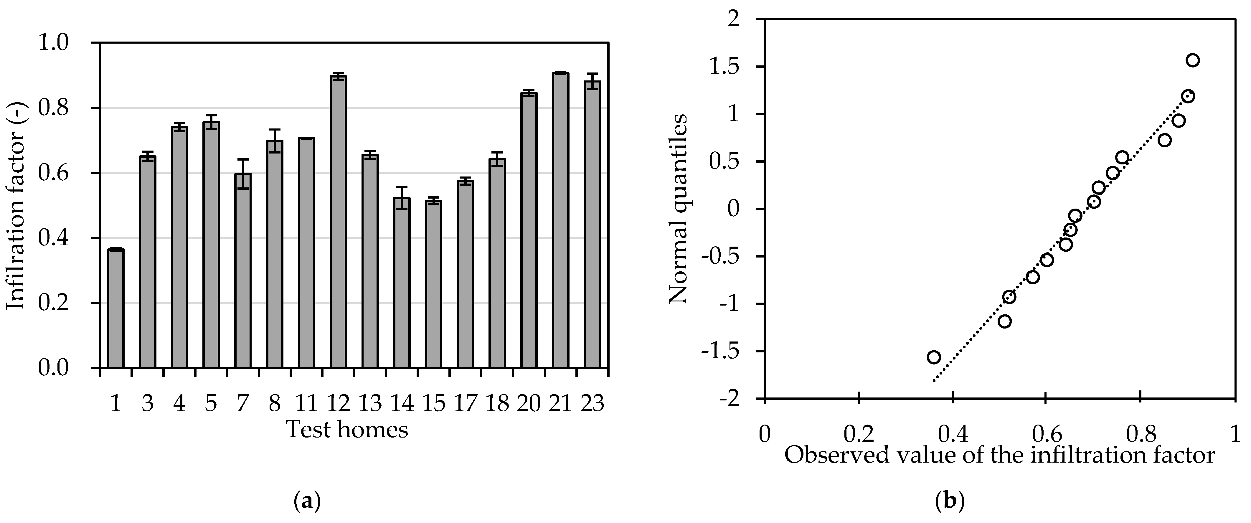
3.2. PM2.5 Infiltration Factor
3.3. Correlation between the PM2.5 Infiltration Factor and Building Factors
3.4. PM 2.5 Infiltration According to
4. Conclusions
- The infiltration analysis was conducted for 23 target units in Korea, and the effective measurement of the infiltration factor for 23 homes was 0.71 (±0.19).
- Analysis of the correlation between building characteristics and the infiltration factor showed that , ELA/FA, and NL had a statistically significant (p < 0.05), strong positive correlation (r = 0.701, 0.685, 0.684) with the infiltration factor.
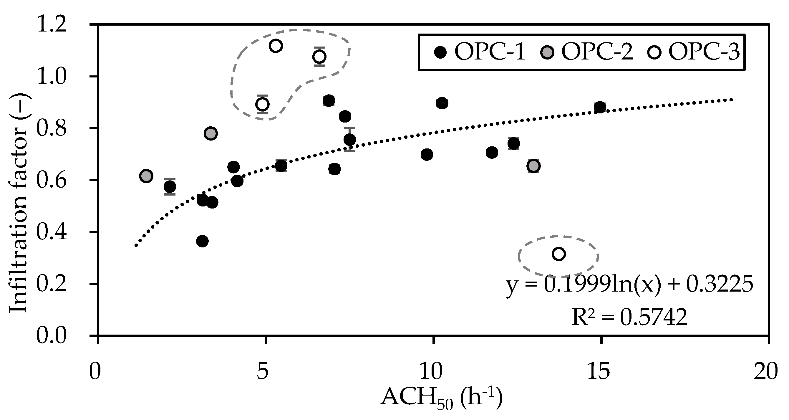
- Based on the correlation analysis, was selected as the dominant predictor for infiltration, and a regression model (0.57) was developed to explain the infiltration rate by the index: = 0.1999 ln() + 0.3225.
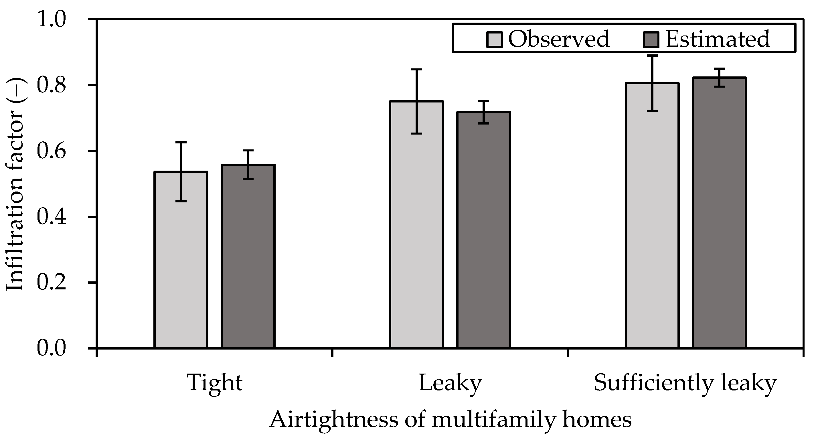
- The analysis of the infiltration rate according to the leakage class confirmed that the concentration of outdoor-origin in sufficiently leaky units can be up to 1.59 times higher than that in tight units.
Author Contributions
Funding
Conflicts of Interest
References
- Brook, R.D.; Rajagopalan, S.; Pope, C.A., 3rd; Brook, J.R.; Bhantnagar, A.; Luepker, R.V.; Mitteleman, M.A.; Peters, A.; Siscovick, D.; Simth, S.C.; et al. Particulate matter air pollution and cardiovascular disease: An update to the scientific statement from the American Heart Association. Circulation 2010, 121, 2311–2378. [Google Scholar] [CrossRef]
- Kim, I.S.; Jang, J.Y.; Kim, T.H.; Park, J.; Shim, J.; Kim, J.B.; Byun, Y.S.; Sung, J.H.; Yoon, T.W.; Kim, J.Y.; et al. Guidelines for the prevention and management of cardiovascular disease associated with fine dust/Asian dust exposure. J. Korean Med. Assoc. 2015, 58, 1044–1059. [Google Scholar] [CrossRef]
- The State Council of the People’s Republic of China. Air Pollution Prevention and Control Action Plan. Available online: http://www.gov.cn/zwgk/2013-09/12/contenst_2486773.htm (accessed on 30 December 2020).
- Liu, D.L.; Nazaroff, W.W. Particle penetration through building cracks. Aerosol Sci. Technol. 2003, 37, 563–573. [Google Scholar] [CrossRef]
- Chen, C.; Zhao, B. Review of relationship between indoor and outdoor particles: I/O ratio, infiltration factor and penetration factor. Atmos. Environ. 2011, 45, 275–288. [Google Scholar] [CrossRef]
- Long, C.; Suh, H.; Kobzik, L.; Catalano, P.; Ning, Y. A pilot investigation of the relative toxicity of indoor and outdoor fine particles: Invitro effects of endotoxin and other particulate properties. Environ. Health Perspect. 2001, 109, 1019–1026. [Google Scholar] [CrossRef]
- Wilson, W.; Brauer, M. Estimation of ambient and non-ambient components of particulate matter exposure from a personal monitoring panel study. J. Expo. Sci. Environ. Epidemiol. 2006, 16, 264–274. [Google Scholar] [CrossRef]
- Ebelt, S.T.; Wilson, W.E.; Brauer, M. Exposure to ambient and nonambient components of particulate matter: A comparison of health effects. Epidemiology 2005, 16, 227–250. [Google Scholar] [CrossRef] [PubMed]
- Clyaton, C.A.; Perritt, R.L.; Pellizzari, E.D.; Thomas, K.W.; Whitmore, R.W.; Wallace, L.A.; Ozkaynak, H.; Spengler, J.D. Particle total exposure assessment methodology (PTEAM) study: Distributions of aerosol and elemental concentrations in personal, indoor, and outdoor air samples in a southern California community. J. Expo. Anal. Environ. Epidemiol. 1993, 3, 227–250. [Google Scholar]
- Fisher, P.H.; Hoek, G.; van Reeuwijk, H.; Briggs, D.J.; Lebret, E.; van Wijnen, J.H.; Kingham, S.; Elliott, P.E. Traffic-related differences in outdoor and indoor concentrations of particles and volatile organic compounds in Amsterdam. Atmos. Environ. 2000, 34, 3713–3722. [Google Scholar] [CrossRef]
- Chao, C.Y.H.; Tung, T.C. An empirical model for outdoor contaminant transmission into residential buildings and experimental verification. Atmos. Environ. 2001, 35, 1585–1596. [Google Scholar] [CrossRef]
- Liu, L.J.S.; Box, M.; Kalman, D.; Kaufman, J.; Koenig, J.; Larson, T.; Lumley, T.; Sheppard, L.; Wallace, L. Exposure assessment of particulate matter for susceptible populations in Seattle. Environ. Health Perspect. 2003, 111, 909–918. [Google Scholar] [CrossRef]
- Lachenmyer, C.; Hidy, G.M. Urban measurements of outdoor-indoor PM2.5 concentrations and personal exposure in the Deep South. Part 1. Pilot study of mass concentrations for nonsmoking subjects. Aerosol Sci. Technol. 2000, 32, 34–51. [Google Scholar] [CrossRef]
- Landis, M.S.; Norris, G.A.; Williams, R.W.; Weinstein, J.P. Personal exposures to PM2.5 mass and trace elements in Baltimore, MD, USA. Atmos. Environ. 2001, 35, 6511–6524. [Google Scholar] [CrossRef]
- Williams, R.; Suggs, J.; Rea, A.; Sheldon, L.; Rodes, C.; Thronburg, J. The research Triangle Park particulate matter panel study: Modeling ambient source contribution to personal and residential PM mass concentrations. Atmos. Environ. 2003, 37, 5365–5378. [Google Scholar] [CrossRef]
- Wallace, L.; Williams, R. Use of personal-indoor-outdoor sulfur concentrations to estimate the infiltration factor and outdoor exposure factor for individual homes and persons. Environ. Sci. Technol. 2005, 39, 1707–1714. [Google Scholar] [CrossRef]
- Meng, Q.Y.; Spector, D.; Colome, S.; Turpin, B. Determinants of indoor and personal exposure to PM2.5 of indoor and outdoor origin during the RIOPA study. Atmos. Environ. 2009, 43, 5750–5758. [Google Scholar] [CrossRef] [PubMed]
- Choi, D.H.; Kang, D.H. Infiltration of ambient PM2.5 through building envelope in apartment housing units in Korea. Aerosol Air Qual. Res. 2017, 17, 598–607. [Google Scholar] [CrossRef]
- Chen, Z.; Chen, C.; Wei, S.; Wu, Y.; Wang, Y.; Wan, Y. Impact of the external window crack structure on indoor PM2.5 mass concentration. Build. Environ. 2016, 108, 240–251. [Google Scholar] [CrossRef]
- MacNeill, M.; Wallace, L.; Kearney, J.; Allen, R.W.; Van Ryswyk, K.; Judek, S.; Xu, X.; Wheeler, A. Factors influencing variability in the infiltration of PM2.5 mass and its components. Atmos. Environ. 2012, 37, 518–532. [Google Scholar] [CrossRef]
- Han, Y.; Qi, M.; Chen, Y.; Shen, H.; Liu, J.; Huang, Y.; Chen, H.; Liu, W.; Wang, X.; Liu, J.; et al. Influence of ambient air PM2.5 concentration and meteorological condition on the indoor PM2.5 concentrations in a residential apartment in Beijing using a new approach. Environ. Pollut. 2015, 205, 307–314. [Google Scholar] [CrossRef]
- Stephens, B.; Siegel, J.A. Penetration of ambient submicron particles into single-family residences and associations with building characteristics. Indoor Air 2012, 22, 501–513. [Google Scholar] [CrossRef]
- Population and Housing Census. Available online: http://www.census.go.kr/dat/ysr/ysrList.do?q_menu=6&q_sub=3 (accessed on 30 December 2020).
- Choi, D.H.; Kang, D.H. Indoor/outdoor relationships of airborne particles under controlled pressure difference across the building envelope in Korean multifamily apartments. Sustainability 2018, 10, 4074. [Google Scholar] [CrossRef]
- ISO. ISO 9972. Thermal Performance of Buildings-Determination of air Permeability of Buildings-Fan Pressurization Method; International Standard Organization: Geneva, Switzerland, 2015. [Google Scholar]
- ASHRAE. ANSI/ASHRAE Standard 119: Air Leakage Performance for Detached Single-Family Residential Buildings; American Society of Heating, Refrigerating & Air Conditioning Engineers: Atlanta, GA, USA, 1998. [Google Scholar]
- Walker, I.S.; Sherman, M.H.; Joh, J.; Chan, W.R. Applying Large datasets to developing a better understanding of air leakage measurement in homes. Int. J. Vent. 2013, 11, 323–337. [Google Scholar]
- Kalamees, T.; Kurnitski, J.; Jokisalo, J.; Eskola, L.; Jokiranta, K.; Vinha, J. Measured and simulated air pressure conditions in Finnish residential buildings. Build. Serv. Eng. Res. Technol. 2010, 31, 177–190. [Google Scholar] [CrossRef]
- Jo, J.H.; Lim, J.H.; Song, S.Y.; Yeo, M.S.; Kim, K.W. Characteristics of pressure distribution and solution to the problems caused by stack effect in high-rise residential buildings. Build. Environ. 2007, 42, 263–277. [Google Scholar] [CrossRef]
- Huang, L.; Hopke, P.K.; Zhao, W.; Li, M. Determinants on ambient PM2.5 infiltration in non-heating season for urban residences in Beijing: Building characteristics, interior surface covering and human behavior. Atmos. Pollut. Res. 2015, 6, 1046–1054. [Google Scholar] [CrossRef]
- Shi, Y.; Li, X.; Li, H. A new method to assess infiltration rates in large shopping centers. Build. Environ. 2017, 119, 140–152. [Google Scholar] [CrossRef]
- Li, Z.; Tong, X.; Ho, J.M.W.; Kwok, T.C.Y.; Dong, G.; Ho, K.; Yim, S.H.L. A practical framework for predicting residential indoor PM2.5 concentration using land-use regression and machine learning methods. Chemosphere 2021, 265, 129140. [Google Scholar] [CrossRef]
- Hauri, D.D.; Huss, A.; Zimmermann, F.; Kuehni, C.E.; Roosli, M. A prediction model for assessing residential radon concentration in Switzerland. J. Environ. Radioact. 2012, 112, 83–89. [Google Scholar] [CrossRef]
- Won, G.H.; Huh, J.H. Airtightness evaluation of apartments based on their deterioration length. In Proceedings of the Society of Air-Conditioning and Refrigerating Engineers of Korea, Seoul, Korea, 21 November 2002; pp. 508–513. [Google Scholar]
- Kwon, O.H.; Kim, J.H.; Kim, M.H.; Seok, Y.J.; Jeong, J.W. Case study of residential building air tightness in Korea based on blower door test approach. J. Archit. Inst. Korea Plan. Des. 2010, 26, 303–310. [Google Scholar]
- Jo, J.H. Measurements of the dwelling unit airtightness in high-rise residential buildings. J. Archit. Inst. Korea Plan. Des. 2010, 26, 337–344. [Google Scholar]
- Yoon, J.O. Field Measurement of infiltration in new apartments using de-pressurization method. Korea Inst. Ecol. Archit. Environ. J. 2013, 13, 27–32. [Google Scholar]
- Lee, S.I.; Kim, J.G.; Kim, S.H.; Kim, J.H.; Jeong, H.G.; Jang, C.Y. An analysis of the airtightness performance and heating energy demand according to building structural characteristics. Korea Inst. Ecol. Archit. Environ. J. 2015, 15, 109–115. [Google Scholar]
- Eisner, A.D.; Richmond-Bryant, J.; Hagn, I.; Drake-Richman, Z.; Brixey, L.A.; Wiener, R.W.; Ellenson, W.D. Analysis of indoor air pollution trends and characterization of infiltration delay time using a cross-correlation method. J. Environ. Monit. 2009, 11, 2201–2206. [Google Scholar] [CrossRef]
- Albuquerque, P.C.; Gomes, J.F.; Bordado, J.C. Assessment of exposure to airborne ultrafine particles in the urban environment of Lisbon, Portugal. J. Air Waste Manag. Assoc. 2012, 62, 373–380. [Google Scholar] [CrossRef] [PubMed]
- Bordado, J.C.; Gomes, J.F.; Albuquerque, P.C. Exposure to airborne ultrafine particles from cooking in Portuguese homes. J. Air Waste Manag. Assoc. 2012, 62, 1116–1126. [Google Scholar] [CrossRef]


| Building Factor | Mean | Standard Deviation | Median | Min. | Max. |
|---|---|---|---|---|---|
| Construction year | 13.6 | 10.8 | 10.0 | 1.0 | 38.0 |
| Floor area (m2) | 57.4 | 48.3 | 36.0 | 14.0 | 212.0 |
| Volume (m3) | 131.4 | 111.2 | 83.0 | 32.0 | 488.0 |
| Exterior wall area (m2) | 30.4 | 20.2 | 21.7 | 7.7 | 68.5 |
| Window area (m2) | 16.1 | 14.9 | 11.8 | 1.8 | 51.6 |
| EWA/FA (1) (-) | 0.62 | 0.27 | 0.54 | 0.25 | 1.19 |
| WA/FA (2) (-) | 0.27 | 0.11 | 0.26 | 0.10 | 0.51 |
| Leakage Class | Maximum NL | Ventilation Requirement | Airtightness | |
|---|---|---|---|---|
| A | 0.1 | 1 | Full | Sufficiently tight |
| B | 0.14 | 2 | Yes | Quite tight |
| C | 0.2 | 3 | Yes | |
| D | 0.28 | 5 | Some | Leaky |
| E | 0.4 | 7 | Likely | |
| F | 0.57 | 10 | Possible | Sufficiently leaky |
| G | 0.8 | 14 | Unlikely | |
| H | 1.13 | 20 | None | - |
| I | 1.6 | 27 | Buildings in this range may be too loose and should be tightened | |
| J | - | - | ||
| Case | |||
|---|---|---|---|
| Average | Standard Deviation | ||
| High level and low fluctuation | ≥35 | <10% of | OPC-1 |
| Low level and low fluctuation | <35 | <10% of | OPC-2 |
| High level and high fluctuation | ≥35 | >10% of | OPC-3 |
| Unit | C (m3·h−1·Pa−n) | N (−) | ELA (cm2) | Specific ELA (cm2/m2) | ACH50 | NL (−) | Leakage Class | ||
|---|---|---|---|---|---|---|---|---|---|
| ELA/EWA | ELA/WA | ELA/FA | |||||||
| 1 | 49.11 | 0.65 | 131 | 2.63 | 3.00 | 1.54 | 3.1 | 0.15 | C |
| 2 | 99.31 | 0.60 | 247 | 4.51 | 5.62 | 1.90 | 3.4 | 0.19 | C |
| 3 | 159.63 | 0.67 | 435 | 6.35 | 8.43 | 2.05 | 4.0 | 0.20 | D |
| 4 | 136.02 | 0.69 | 381 | N. A. | N. A. | 6.69 | 12.4 | 0.64 | G |
| 5 | 58.31 | 0.60 | 144 | 7.84 | 14.15 | 4.01 | 7.5 | 0.39 | E |
| 6 | 47.24 | 0.63 | 121 | 13.49 | 23.19 | 3.36 | 6.6 | 0.33 | E |
| 7 | 70.82 | 0.66 | 191 | 4.20 | 8.94 | 2.25 | 4.2 | 0.22 | D |
| 8 | 81.94 | 0.59 | 200 | 10.86 | 27.94 | 5.55 | 9.8 | 0.54 | F |
| 9 | 2.53 | 0.82 | 8 | 0.63 | 4.69 | 0.47 | 1.4 | 0.05 | A |
| 10 | 149.88 | 0.62 | 379 | 6.24 | 14.06 | 2.65 | 4.9 | 0.26 | D |
| 11 | 144.13 | 0.57 | 343 | 12.42 | 25.59 | 6.85 | 11.7 | 0.67 | G |
| 12 | 38.24 | 0.63 | 98 | 5.06 | 36.24 | 4.89 | 10.3 | 0.47 | F |
| 13 | 89.15 | 0.57 | 212 | 4.21 | 11.92 | 3.26 | 5.5 | 0.32 | E |
| 14 | 14.60 | 0.74 | 44 | 1.38 | 3.13 | 1.21 | 3.1 | 0.12 | B |
| 15 | 13.82 | 0.77 | 43 | 1.35 | 3.08 | 1.19 | 3.4 | 0.12 | B |
| 16 | 124.86 | 0.60 | 310 | 12.91 | 21.91 | 7.01 | 13.0 | 0.68 | G |
| 17 | 8.45 | 0.77 | 26 | 2.65 | 4.40 | 0.76 | 2.1 | 0.07 | A |
| 18 | 100.91 | 0.67 | 273 | 4.01 | 7.74 | 3.25 | 7.0 | 0.32 | E |
| 19 | 68.92 | 0.70 | 194 | 13.52 | 36.33 | 5.87 | 13.7 | 0.57 | G |
| 20 | 32.78 | 0.58 | 79 | 4.45 | 15.26 | 4.91 | 7.4 | 0.48 | E |
| 21 | 18.71 | 0.67 | 51 | 2.66 | 8.59 | 3.17 | 6.9 | 0.31 | D |
| 22 | 13.31 | 0.65 | 35 | 4.56 | 14.03 | 2.51 | 5.3 | 0.24 | D |
| 23 | 85.95 | 0.62 | 220 | 27.29 | 30.94 | 7.65 | 15.0 | 0.75 | G |
| Unit | |||||||||
|---|---|---|---|---|---|---|---|---|---|
| Average | Standard Deviation | Average | Standard Deviation | Average | Standard Deviation | Average | Standard Deviation | ||
| 1 | 142 | 14 | 169 | 2 | 62 | 0 | 0.36 | 0.00 | OPC-1 |
| 2 | 27 | 1 | 26 | 0 | 20 | 0 | 0.78 | 0.01 | OPC-2 |
| 3 | 159 | 4 | 160 | 4 | 104 | 1 | 0.65 | 0.01 | OPC-1 |
| 4 | 77 | 2 | 78 | 4 | 58 | 1 | 0.74 | 0.02 | OPC-1 |
| 5 | 35 | 1 | 34 | 1 | 26 | 1 | 0.76 | 0.04 | OPC-1 |
| 6 | 66 | 7 | 63 | 1 | 68 | 1 | 1.08 | 0.04 | OPC-3 |
| 7 | 132 | 3 | 133 | 1 | 79 | 1 | 0.60 | 0.00 | OPC-1 |
| 8 | 53 | 2 | 53 | 1 | 37 | 0 | 0.70 | 0.01 | OPC-1 |
| 9 | 34 | 1 | 35 | 0 | 21 | 0 | 0.62 | 0.01 | OPC-2 |
| 10 | 102 | 11 | 86 | 2 | 76 | 2 | 0.89 | 0.03 | OPC-3 |
| 11 | 189 | 10 | 192 | 2 | 135 | 1 | 0.71 | 0.01 | OPC-1 |
| 12 | 35 | 2 | 35 | 1 | 32 | 0 | 0.90 | 0.01 | OPC-1 |
| 13 | 75 | 4 | 70 | 2 | 46 | 1 | 0.66 | 0.02 | OPC-1 |
| 14 | 130 | 2 | 133 | 0 | 70 | 1 | 0.52 | 0.01 | OPC-1 |
| 15 | 266 | 25 | 296 | 1 | 152 | 1 | 0.51 | 0.00 | OPC-1 |
| 16 | 30 | 1 | 30 | 1 | 20 | 0 | 0.65 | 0.02 | OPC-2 |
| 17 | 41 | 3 | 43 | 1 | 25 | 0 | 0.57 | 0.03 | OPC-1 |
| 18 | 74 | 2 | 76 | 1 | 49 | 1 | 0.64 | 0.02 | OPC-1 |
| 19 | 82 | 9 | 94 | 2 | 30 | 1 | 0.31 | 0.01 | OPC-3 |
| 20 | 91 | 1 | 90 | 1 | 76 | 0 | 0.85 | 0.01 | OPC-1 |
| 21 | 51 | 3 | 52 | 1 | 47 | 0 | 0.91 | 0.01 | OPC-1 |
| 22 | 44 | 4 | 41 | 0 | 46 | 0 | 1.12 | 0.01 | OPC-3 |
| 23 | 70 | 3 | 73 | 2 | 64 | 1 | 0.88 | 0.01 | OPC-1 |
| Normality Test | Degrees of Freedom | t | p-Value |
|---|---|---|---|
| Kolmogorov–Smirnov | 16 | 0.107 | 0.200 * |
| Shapiro–Wilk | 16 | 0.965 | 0.755 * |
| Year of Construction | Floor Area | Volume | EWA/FA | WA/FA | ELA/FA | ACH50 | NL | Fin | |
|---|---|---|---|---|---|---|---|---|---|
| Construction year | 1.000 | 0.122 | 0.112 | −0.473 | −0.300 | 0.604 * | 0.561 * | 0.598 * | 0.341 |
| Floor area | 0.122 | 1 | 0.999 ** | −0.433 | 0.052 | −0.287 | −0.311 | −0.287 | −0.362 |
| Volume | 0.112 | 0.999 ** | 1.000 | −0.434 | 0.057 | −0.295 | −0.319 | −0.295 | −0.366 |
| EWA/FA | −0.473 | −0.433 | −0.434 | 1.000 | 0.369 | −0.083 | −0.082 | −0.082 | 0.257 |
| WA/FA | −0.300 | 0.052 | 0.057 | 0.369 | 1.000 | −0.362 | −0.354 | −0.353 | −0.489 |
| ELA/FA | 0.604 * | −0.287 | −0.295 | −0.083 | −0.362 | 1.000 | 0.979 ** | 0.999 ** | 0.685 ** |
| ACH50 | 0.561 * | −0.311 | −0.319 | −0.082 | −0.354 | 0.979 ** | 1.000 | 0.978 ** | 0.701 ** |
| NL | 0.598 * | −0.287 | −0.295 | −0.082 | −0.353 | 0.999 ** | 0.978 ** | 1.000 | 0.684 ** |
| Fin | 0.341 | −0.362 | −0.366 | 0.257 | −0.489 | 0.685 ** | 0.701 ** | 0.684 ** | 1.000 |
| Building Characteristic | Correlation Coefficient (r) | p-Value | Rank |
|---|---|---|---|
| ACH50 | 0.701 | 0.002 ** | 1 |
| ELA/FA | 0.685 | 0.003 ** | 2 |
| NL | 0.684 | 0.003 ** | 3 |
| WA/FA | −0.489 | 0.064 | 4 |
| Volume | −0.366 | 0.163 | 5 |
| Floor area | −0.362 | 0.168 | 6 |
| Construction year | 0.341 | 0.196 | 7 |
| EWA/FA | 0.257 | 0.354 | 8 |
| Regression Model | Equation | α | β | R2 |
|---|---|---|---|---|
| Linear | 0.485 ** | 0.028 ** | 0.50 | |
| Log–Linear | 0.322 ** | 0.200 ** | 0.57 | |
| Linear–Log | −0.715 ** | 0.044 ** | 0.48 | |
| Log–Log | −0.972 ** | 0.314 ** | 0.56 |
Publisher’s Note: MDPI stays neutral with regard to jurisdictional claims in published maps and institutional affiliations. |
© 2021 by the authors. Licensee MDPI, Basel, Switzerland. This article is an open access article distributed under the terms and conditions of the Creative Commons Attribution (CC BY) license (https://creativecommons.org/licenses/by/4.0/).
Share and Cite
Park, B.R.; Eom, Y.S.; Choi, D.H.; Kang, D.H. Estimation of Outdoor PM2.5 Infiltration into Multifamily Homes Depending on Building Characteristics Using Regression Models. Sustainability 2021, 13, 5708. https://doi.org/10.3390/su13105708
Park BR, Eom YS, Choi DH, Kang DH. Estimation of Outdoor PM2.5 Infiltration into Multifamily Homes Depending on Building Characteristics Using Regression Models. Sustainability. 2021; 13(10):5708. https://doi.org/10.3390/su13105708
Chicago/Turabian StylePark, Bo Ram, Ye Seul Eom, Dong Hee Choi, and Dong Hwa Kang. 2021. "Estimation of Outdoor PM2.5 Infiltration into Multifamily Homes Depending on Building Characteristics Using Regression Models" Sustainability 13, no. 10: 5708. https://doi.org/10.3390/su13105708
APA StylePark, B. R., Eom, Y. S., Choi, D. H., & Kang, D. H. (2021). Estimation of Outdoor PM2.5 Infiltration into Multifamily Homes Depending on Building Characteristics Using Regression Models. Sustainability, 13(10), 5708. https://doi.org/10.3390/su13105708