Abstract
The analysis of the local regulation effects is required for sustainable and effective land utilization because land use/land cover (LULC) changes are not only determined by human activity but are also affected by national policy and regulation; however, previous studies for land use/land cover (LULC) have mainly been conducted on the LULC changes using past experience. This study, therefore, analyzed the effects of local regulations aimed at preserving the water quality in South Korea. To this end, changes in LULC were simulated using the CA-Markov model under conditions in which two local regulations, the special countermeasure area (SCA) and total maximum daily load (TMDL), were not applied and examined the differences between the simulated LULC and the actual LULC as of 2018. In addition, the differences in the generation of pollutant loads were driven for Biochemical Oxygen Demand (BOD), Total Nitrogen (TN), and Total Phosphorus (TP) using pollutant unit-load. As a result, without SCA, the agricultural area increased by 379.0 km2, the urban area decreased by 101.8 km2, and the meadow area decreased by 176.0 km2. In addition, without TMDL, the urban area increased by 169.2 km2 and the meadow area decreased to 158.8 km2.Differences in BOD, TN, and TP pollution loads without SCA applications were shown to decrease to 22,710.5 kg·km−2 day−1, 1133.9 kg·km−2 day−1, and 429.8 kg·km−2 day−1, respectively, while BOD, TN, and TP pollution loads without TMDL applications decreased to 14,435.7 kg·km−2 day−1, 2543.6 kg·km−2 day−1, and 368.2 kg·km−2 day−1, respectively. As such, this study presents a methodology for analyzing the effects of local regulations using the CA-Markov model, which can intuitively and efficiently examine the effects of regulations by predicting LULC changes.
1. Introduction
Land use/land cover (LULC) is changing worldwide as a result of radical industrialization, with large tracts of natural land undergoing rapid transformation into agricultural or urban land under the influence of political, economic, social, and cultural requirements [1,2]. LULC changes (LUCC) generally result from the unnatural activities of human beings [3], and the term implies that natural land has been disturbed by human activity. Disturbance of natural land that is caused by LUCC can lead to environmental problems such as frequent flooding [4,5] or a decline in the quality of a water body [6,7,8]. In this regard, a review of the environmental effects of LUCC is required in the process of establishing plans for sustainable LUCC [9].
Accordingly, significant effort has been made in many countries to stably manage the quality of their main water resources. As changes in the LULC near water resources can lead directly to water pollution, many countries have implemented schemes to minimize regional development in areas where LUCC are expected via local regulation. The implementation of local regulations in the Paldang watershed is an example of LULC control in South Korea. The Paldang watershed refers to seven cities and counties that surround Paldang Lake, which is located on the eastern side of Seoul, the capital of South Korea. The lake is regarded as a crucial resource as it supplies water to approximately 50% (approximately 25 million) of the total population in South Korea. The conditions surrounding the water resources in this area are particularly rare even on a global scale, and the Korean government has adopted strict local regulations for the Paldang watershed to manage water pollution and encourage satisfactory and stable conditions in the lake. As Paldang Lake is considered one of the most important resources in South Korea the central government has prioritized the management of its water quality via policy making [10]. The national objective for the water quality in Paldang Lake has been designated 1 mg/L based on the biochemical oxygen demand (BOD) to ensure the stability of the water quality in the lake from the perspective of security. The Paldang watershed was designated an area for special countermeasures (SCA) in 1990 and a system for managing the total water pollution, or the total maximum daily load (TMDL) has been implemented in the area by restricting development and managing the amount of water pollutants reaching the lake since 2013.
However, local regulations have also led to negative results. The Paldang watershed is very close to Seoul, the capital of South Korea, and there is a high level of pressure for regional development in the area. The local regulations established by the Korean government in the Paldang watershed to preserve the water quality in this region have reduced the welfare and the quality of life for the local residents. As the local regulations suppress the significant demand for regional development in the Paldang watershed, an increasing number of residents that live in this region are protesting against the regulations. To respond to this resistance, the central government needs to verify the positive effects of these regulations with scientific methods, encourage the active participation of the residents in preserving the water quality in the watershed, which is the ultimate objective of the Korean government, and provide enhanced and logical compensation for residents that have been affected by the regulations. However, the Korean government has failed to present any data that can verify the efficacy of the regulations, and this lack of evidence has accelerated the formation of public opinion affirming the uselessness of the regulations.
With regard to these circumstances, research on the environmental effects of LUCC is required. Previous research that has examined these effects includes a study by Sarah Hasan et al. [11] in which the future radical urbanization of the southern regions in China was predicted using remote sensing data and concerns were expressed about the level of urbanization expected based on the results. Hamad et al. [12] predicted the LULC in the Halgurd-Sakran Core Zone of Iraq in 2013 by establishing two scenarios based on LandSat 5 images and the CA-Markov model and reported that accurate predictions about the LULC were made when the image data utilized described a period that was temporally close to that used in the simulation. Salem et al. [13] analyzed the driving forces of urbanization by considering LUCC, and Ansari and Golabi [14] predicted spatial changes in the desert wetlands of Iran. As such, most of the previous studies have been mainly conducted on land utilization change due to natural conditions and urban area expansion due to industrialization. However, although land use in a country frequently leads to substantial LULC control through government regulations, previous studies rarely considered the influence of regulations on LULC. In summary, LULC changes caused by regulations, as well as the effects of natural conditions and industrialization, must be continually assessed in order to continue efficient LULC.
Thus, this study focused on the Paldang watershed, which is the main water resource in South Korea, as a research target and simulated the LUCC visually in the area under conditions in which the local regulations were not applied. This study presented the difference of pollutant load change using pollutant unit-loads under the same conditions. Through these attempts, this study would like to suggest that this methodology could play a role as a decision-making tool for the field of sustainable and efficient LULC planning.
2. Materials and Methods
2.1. Study Area
Paldang watershed, the area to be investigated in this study, comprises seven cities and counties (Gapyeong county, Gwangju city, Namyangju city, Yangpyeong county, Yeoju city, Yongin city, and Icheon city) that lie near Paldang Lake. As shown in Figure 1, three rivers (Namhan River, Bukhan River, and Gyoungan River) flow into Paldang Lake via the watershed. For this reason, the water quality of Paldang Lake cannot be maintained if water pollution occurs as a result of LUCC in the Paldang watershed. The central government limits the LULC changes in the Paldang watershed to the maximum at which water pollution can be prevented. These governmental restrictions mean that the Paldang watershed is less affected by LUCC than other capital areas. The region targeted for this study comprises 61.2% forest and 18.6% agricultural land. As urban areas account for only 5.8% of the entire region, the urban area is significantly smaller than the forested and agricultural areas (Table 1).
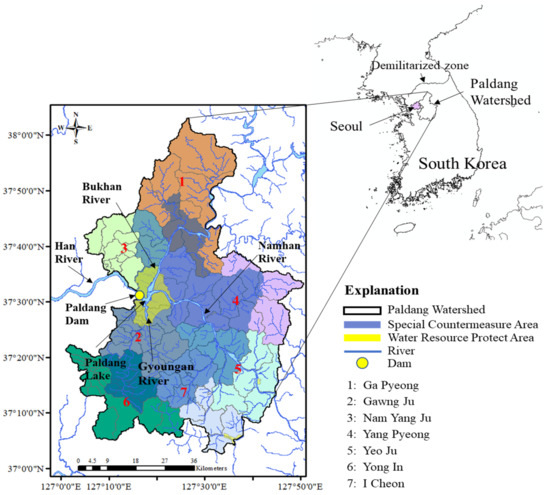
Figure 1.
Scheme of the study area.

Table 1.
Composition and description of LULC in the study area.
2.2. Data Collection
This study utilized data describing the LULC in the study area with the digital elevation model (DEM), road maps, and slope. The LULC map was sourced from the website associated with the Environmental Geographic Information Service (EGIS) [15]. This map, which is produced by the Ministry of Environment (ME) in South Korea, is provided to the public as an online open-source resource to promote active research. The LULC maps are classified as large, medium, and small and include 7, 22, and 41 LULC items, respectively. This study utilized the large LULC map that includes seven environmental parameters; urban, agricultural, mixed forest, meadow, wetland, barren, and water. The LULC map produced by EGIS is represented in the form of raster data according to the mapping guidelines for land coverage maps (Order no. 1317) that were formulated by the ME. The guidelines that were used to create the LULC map state that the following six stages should be used to produce the map. First, primary land coverage classification is carried out using a video classification method that is based on data such as videos, digital maps, and a stock map that is related to a particular region to form the LULC map. Second, secondary land coverage classification is implemented by comparing the video data with the reference data based on the result obtained through the primary land coverage classification. Third, errors are corrected by comparing the LULC classification results with the video data and the quality is inspected using the comparison data. Fourth, if the previous analyses are unlikely, a field investigation is carried out and the result of this investigation is used to produce the LULC map. Fifth, the LULC classification result is sampled, and the result is compared with the video data for verification. Several previous studies have examined the reliability of LU classification using the Kappa coefficient [16,17], whereas the ME evaluates the accuracy of the classification (AC) with Equation (1). Sixth, the final accuracy of the classification (FAC) is calculated using Equation (2). When the FAC is calculated at 95% or higher, the result is provided online. When it is below the standard, quality inspections and corrections are repeated for re-evaluation.
where N is the number of samples obtained from the LULC classification result, is the number of errors found in the samples used for classification, i is a classification item used in the LULC map, and N is the number of classification items used in the LULC map. Data describing the DEM were collected from the website from the Water Resources Management Information System (WAMIS) [18], and those detailing the road map were collected from the website of the National Transport Information Center (NTIC) [19]. Table 2 shows the data used in this study, and Figure 2 shows examples of data.
Table 2.
Description of the LULC, digital elevation model, and the road map.
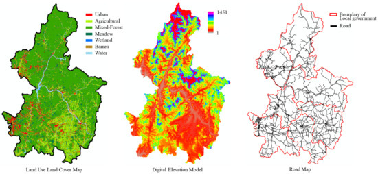
Figure 2.
Images showing the LULC, digital elevation model, and the road map.
3. Methodology
3.1. Major Local Regulations and Design of Effectiveness Analysis
As mentioned in the Introduction, the local regulations that are implemented in the study area require consideration to analyze the effects that local regulations have on LUCC prediction. The water resource protection area (WRPA) in the study area was first established and applied in 1975, the SCA was created in 1990, comprehensive measures for Han River were established in 1998, and the TMDL system was put in place in 2013. The WRPA covers a total of 158.8 km2, includes Paldang Lake and the areas surrounding Paldang Lake, and accounts for 3.7% of the entire Paldang watershed. The SCA is 2096.5 km2 in size and accounts for 49.2% of the entire Paldang watershed. The TMDL system covers the entire Paldang watershed.
As the WRPA that was originally protected occupied a very small proportion of the entire Paldang watershed, it did not have a direct impact on the development of the Paldang watershed. Furthermore, the SCA was no more than a declarative concept when it was first designed in 1990. However, when the water quality of the Han River (BOD 2.0 mg/L) was found to have deteriorated in 1998, public opinion moved toward conserving the water quality. Accordingly, the central government announced comprehensive measures for the Han River in 1998, and local regulations associated with its designation as the SCA was practically adopted in 1999. Since then, the SCA system has been the strictest regulation applied to the Paldang watershed, prohibiting the establishment of factories, livestock facilities, golf courses, mines, and collective cemeteries in this region and restricting the size of residential facilities and facilities that are to be used for hospitality. In addition, the sewage treatment plants in the Paldang watershed are set to perform water treatment based on a BOD of 10 mg/L or less.
The paradigm of water quality management in South Korea changed from qualitative management to quantitative management in the late 2000s. In accordance with these changes, the TMDL system was initiated in the Paldang watershed in 2013 and has been more strictly applied in this region than it has in the rest of Korea. The regulations have interrupted the regional development of the Paldang watershed, with sewage treatment plants required to perform water treatment based on a BOD of 5 mg/L or less.
With regards to the changes in the local regulations that have been applied to the Paldang watershed over time, the following assumptions were established in this study. First, the regulations associated with the SCA and the TMDL were established as local regulations for examination. Although the designation of the site as a SCA occurred in 1990, the effects were not observed until 1999. As mentioned above, the TMDL system was implemented in 2013. As these regulations were adopted in different years, the effects of these regulations need to be examined alongside the time difference. Figure 3 shows the concept of how the effects of these local regulations have changed over time.
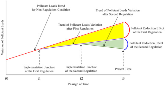
Figure 3.
Conceptual diagram of regulatory effectiveness.
The red line in Figure 3 indicates the amount of water pollution that would reach the lake if local regulations were not implemented. The purple line indicates the change in the water pollution that results from the initial regulations. The green line indicates the change in water pollution that is caused by the second round of regulations. If these conditions are applied to the study area, t1 on the x axis of the figure refers to the year 1999 when the SCA regulations were executed, t2 refers to 2013 when the TMDL regulations were executed, and t3 is the present. Based on these assumptions, the red arc implies the effects of the SCA regulation and the blue arc denotes the effects of the TMDL regulations.
This study established the year 2018 (t3 on the x axis in Figure 3) as the present time and performed a simulation of the LUCC in the Paldang watershed for 2018 under conditions in which the local regulations were not applied. LULC maps from 1989 (t0 on the x axis in Figure 3) and 1999 (t1 on the x axis in Figure 3) were utilized to simulate the LULC for 2018 without the SCA regulation. LULC maps from 1999 (t1 on the x axis in Figure 3) and 2013 (t2 on the x axis in Figure 3) were utilized to simulate the LULC in 2018 with no TMDL regulations applied. The simulated LULC maps and the present LULC map were then compared to analyze the effects of the local regulations.
Conceptual models, such as the Soil Water Assessment Tool [20], the Agricultural Non-Point Source Pollution Model [21], the Storm Water Management Model [22], and the Areal Non-point Source Watershed Environment Response Simulation [23], can be used to examine changes in the amount of water pollutants present within a water body as a result of LUCC. However, these conceptual models cannot directly calculate the water pollutant loads that are generated purely as a result of LUCC because information about the rate at which water pollutants are delivered, self-purification processes, and the effects of sewage treatment plants would be required. To solve this problem, this study applied pollutant unit-loads that are used to describe water pollutants by the Korean government in the establishment of TMDL plans, as they can provide information about the changes in the amount of water pollutants that are caused as a result of LUCC. Pollutant unit-loads have been used in several countries as they can be applied in the simple estimation of water pollutant loads when practical measurement is difficult [24,25]. The Korean government also recommends using this unit in regions where insufficient data has been collected for TMDL planning. The ME has presented pollutant unit-loads that are based on measurement and analyses conducted in several basins in South Korea under the guidelines for TMDL management technology [26], as indicated in Table 3. In this study, analysis of the difference in the water pollutant loads that are associated with LUCC is based on the pollutant unit-loads per area that are generated on a daily basis.
Table 3.
Pollutant unit-loads by LULC.
3.2. LUCC Prediction
3.2.1. CA-Markov Model
This study utilized the CA-Markov model to predict LUCC. The CA-Markov model uses a transition probability matrix (TPM) that is affected by both the Markov chain and cellular automata (CA) [3]. The model has recently been applied in the prediction of future LULC [27,28,29] and has also been adopted for use with various LULC modeling tools and techniques as it can be used effectively in simulations that concern spatial and temporal changes [30]. Generally, the TPM serves as the core element affecting the prediction of LULC [31].
The Markov chain model specifies the spatial changes that occur between two different points in time—t1 and t2—and determines the spatial change tendency as a probability [32,33]. This model has empirical properties and can be applied to LUCC to represent changes that occur in the form of the TPM, which is expressed using Equation (3). The TPM determines the LUCC generated and is close to 0 when the probability of transition decreases and closer to 1 as the probability of transition increases. Moreover, the Markov chain can present a change in LULC over a specific time period that can be used for prediction [34], as shown in Equation (4).
where is a particular condition at time t, and denotes the condition at time [35]. In this study, t was set to represent the LU during a previous period and was set to represent the LULC conditions in the subsequent period.
The CA model is a bottom-up dynamic model that integrates temporal and spatial dimensions with model directions [36]. An important characteristic of this model is that complex processes can be simulated, including discrete time-space systems [37]. Because of this characteristic, the CA model has been widely used in LU simulations [38]. The conditions within each cell of the CA model differ depending on the time-space conditions in adjacent (contiguous) cells [39]. A region that is close to an existing region with a similar category is more likely to be transferred to another category [40]. The CA model comprises parameters such as cells, cell space, neighbors, rules, and time. Neighbors are identified based on the filter used. The value of a weight factor increases as the distance between the central cell and its neighbor decreases. The CA model can be expressed using Equation (5).
where S is the set of conditions in a finite cell, and t and t + 1 indicate the previous and subsequent periods, respectively. n is a neighbor of the cell, and f is a function that denotes the transition regulations in regional space.
The CA model converts any changes in conditions to the Markov transition regulation while also considering previous conditions that are based on an adjacent (contiguous) neighbor. In this study, the standard contiguity filter (5 × 5 matrix) was applied with the CA model, as shown in Equation (6).
3.2.2. Land Change Prediction and Validity Review
This study utilized the Land Change Modeler (LCM) [41] developed by TerrSet to perform the simulation of LUCC. The LCM is based on the CA-Markov model and requires two stages for the prediction of LUCC. In the first stage, the TPM is estimated using the Markov chain. In the second stage, the estimated TPM is reflected in the CA model to simulate the changes in LULC.
1. TPM
The LCM uses the back-propagation neural network (BNN), logistic regression (LogiReg), and the similarity-weighted instance-based machine learning tool (SW) to perform transition potential mapping for TPM estimation [42,43]. Each TPM is estimated by establishing sub-models in the process of predicting LUCC for multiple LULC maps. It can also be used to simulate LUCC based on the TPM of an entire sub-model.
The LCM requires data about the DEM, SLOPE, distance from roads, distance from urban areas, and the distance from water bodies for TPM estimation to produce a LULC map in which the bias between t1 and t2 does not change. It provides variable transformation utility as a tool for removing bias in a transformed LULC map and allows users to use the six functions, namely, evidence likelihood, exponential, square root, natural log, logit, and power.
This study utilized the evidence likelihood function to estimate the TPM based on BNN, which can be used to divide sub-models into groups. This function is generally used to remove bias in the LULC map. It can also derive excellent performance for transition potential mapping based on its high level of efficiency in terms of distributed processing and goodness of fit [44].
2. Prediction of LULC
The TPMs of all the sub-models were used to calculate LUCC, with 2018 as the reference year simulated. As mentioned in Section 3.1, the LULC map in 2018 was simulated by applying two conditions to analyze the effects of the regulations, with the LULC map for the years 1989 and 1999 used for the first condition, and the LULC map for 1999 and 2013 applied as the second. The LULC map for the year 2018 was initially applied with the first condition, followed by the application of the second condition. The results obtained through practical measurement were denoted P-LULC1989–1999, P-LULC1999–2013, and LULC2018.
3. Validity Review
Generally, the validity of the LULC map is confirmed based on the Kappa coefficient [45] between the measured LULC map and the predicted or the ROC curve [13]. However, the Kappa coefficient and the ROC curve are inappropriate for confirming the validity of the LULC map in this study as it aims to predict LUCC alongside local regulations and to compare the LULC conditions of the target time with the present.
To solve this problem, this study proposed a method for confirming the validity of the LULC map based on accuracy, training the root mean square (RMS), and testing the RMS, which can be obtained through BNN training. Of these values, accuracy is the best metric with which to verify the strength of the transition potential mapping and generalize the neural network model. Generally, accuracy is expressed in a range from 0 to 1. Higher accuracy indicates the better performance of a model.
The validity of a model can be determined based on the results of BNN training and testing. Clear determination cannot be performed due to the specific standards that are established. However, a stable decrease in training and testing changes indicates a decrease in problems of over-fitting, which frequently occur in neural networks. In other words, a satisfactory level of prediction in neural networks can be ensured [46,47].
This study, therefore, examined the validity of the BNN model based on the results of calculating accuracy, training the RMS, and testing the RMS in the BNN model. Figure 4 shows the research procedures that were used to analyze the effects of local regulations based on the CA-Markov model.
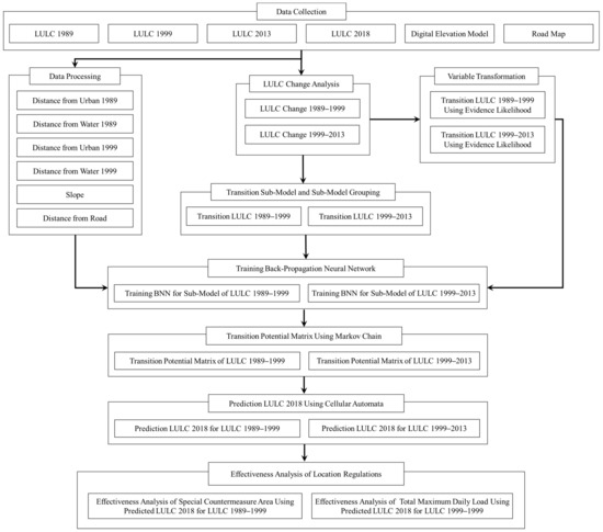
Figure 4.
Overview of this study.
4. Results and Discussion
4.1. Land Changes during 1989–1999 and 1999–2013 and the Transition Sub-Model
Table 4 shows the LUCC from 1989 to 1999, which affected 998.4 km2 with active land transformation observed in the agricultural land, mixed forests, and meadows. The amount of agricultural land increased by 86.0 km2 between 1989 and 1999, which is the largest increase observed in the study area, while the greatest decrease was observed in the mixed forests, which shrunk by 141.4 km2. It was also found that 32.4 km2 of the agricultural land significantly contributed to the increase in urbanization and that 98.4 km2 of mixed-forest land significantly contributed to the increase in agricultural land during the same period. This analysis indicates that the mixed-forest area was mainly developed for use in both urbanization and agriculture in the study area from 1989 to 1999.
Table 4.
Losses, gains, and contributors to net changes during the period 1989–1999.
Table 5 shows the LUCC from 1999 to 2013, which indicates the active land transformation of the agricultural and mixed-forest areas. This result is similar to the results for the period 1989 to 1999. However, the net change in LUCC from 1999 to 2013 includes a decrease in the amount of agricultural and mixed-forest areas by −164.9 km2 and −189.7 km2, respectively, while the urban area increased by 237.2 km2. Agriculture lost 129.3 km2 and mixed-forest lost 72.9 km2 to urbanization. This increase in urbanized land that resulted from the development of agricultural and mixed-forest areas differs significantly from the situation in 1989 to 1999.
Table 5.
Losses, gains, and contributors to the net changes during 1989–1999.
The LCM creates transition sub-models according to the number of conversions that occur for each LULC item. The maximum number of transition sub-models is equal to the number of LULC items multiplied by the number of LULC items minus one. For example, when the number of LULC items is n, the maximum number of LULC items is equal to n(n − 1), which is also relevant when a large number of LULC items are included. The BNN training becomes inefficient when it is directly reflected in the TPM estimation. Thus, the LCM groups the transition sub-models to increase the efficiency of the TPM estimation.
In this study, land changes are observed for all the LULC items, both from 1989 to 1999 and from 1999 to 2013. Therefore, the number of transition sub-models from 1989 to 1999 and 1999 to 2013 was calculated at 42, which were separated into seven groups as shown in Table 6. These groups were then used to estimate the TPM for each model.
Table 6.
Grouping of the Transition Sub-Models for LCM in this study.
4.2. Result of the BNN and TPM
As mentioned above, BNN, LogiReg, and SW are used in the transition potential mapping of each transition sub-model to estimate the TPM. This study utilized BNN because this method can reflect the entire group of variables simultaneously. Before BNN training, parameters such as hidden layer (HL), learning rate (LR), momentum factor (MF), sigmoid constant (SC), and iteration (ITER) need to be established. BNN training was with the HL, LR, MR, SC, and ITER for the transition sub-models at 9, 0.0001, 0.5, 1.0, 1, and 20,000, respectively.
The validity of the model using BNNs is largely determined by two metrics. The first is “whether the model has been learned smoothly”, and the second is “results on unexperienced inputs”. In this work, Training RMS corresponds to the first metric and Test RMS and Accuracy to the second metric. In general, if Test RMS appears to be lower than Training RMS, this phenomenon is judged to be overfitting, which means that overfitting results in poor performance on new or unexperienced data due to excessive learning. That is, stable model performance cannot be guaranteed if overfitting exists.
Table 7 shows the result of RMS, the training RMS of the 1989–1999 transition sub-model ranged from 0.2206 to 0.2496 while the test RMS ranged from 0.2201 to 0.2547. The training RMS of the 1999–2013 transition sub-model ranged from 0.2145 to 0.2496 and the test RMS ranged from 0.2201 to 0.2547. The training RMS of all the transition sub-models was, therefore, higher than the test RMS for all models. If the test RMS is lower than the training RMS, over-fitting is assumed to have occurred, which describes the situation where the performance of a model in analyzing new data is reduced due to excessive learning. In other words, stable model performance cannot be ensured when over-fitting is observed. The results of the training RMS and the test RMS obtained for the 1989–1999 and 1999–2013 transition sub-models in this study do not demonstrate over-fitting. Therefore, it can be assumed that the model training performed well in this study.
Table 7.
Results of back-propagation neural network training.
Furthermore, in predicting land-use changes, minimization of Accuracy is critical [48], and when Accuracy’s results are around 80%, we judge that the model produces good results for unexperienced inputs [31]. Table 7 shows the result of BNN training for 1989 to 1999 based on the transition sub-model and the BNN parameters. The accuracy of the transition sub-model for 1989 to 1999 was in the range of 0.7578–0.9367. Mixed-Forest_TS was the least accurate, whereas Water_TS was the highest. The accuracy of the transition sub-model from 1999 to 2013 was in the range of 0.7508–0.8764, with Urban_TS showing the lowest accuracy and Urban_TS the highest accuracy.
With regard to the results of previous studies, Mishra et al. [31] used remote sensing data to predict the LU in Muzaffarpur, India, and reported an accuracy of 0.5080 for BNN training (HL: 7, LR: 0.0005, MF: 0.5, SC: 1.0, Iter: 10,000). A study by e Silva et al. [49] reported an accuracy of 0.8969 for BNN (ITER; 10,000) in the Taperoa River basin of Brazil. Hasan et al. [11] simulated LU changes by using BNN to simulate the rapid urbanization of southern China and reported an accuracy of 0.7000 or higher for BNN. Pérez-Vega et al. [50] conducted BNN training to identify the TPMs of a recovering sub-model, deforestation sub-model, and perturbation sub-model and reported an accuracy of 0.5920, 0.3520, and 0.5960 for each model, respectively. Oñate-Valdivieso and Bosque Sendra [51] reported a total accuracy of 0.7000 or higher for BNN training. Xiao et al. [52] used GIS and remote sensing (RS) to assess changes in urban expansion and LUCC in China and reported accuracy of 85% and 88% for two testing datasets. Hassan et al. [53] also implemented a classification of Islamabad Pakistan LULC with an accuracy of 89%. In addition, Kogo et al. [54] (2021) employed GIS to analyze the spatiotemporal LULC changes in Western Kenya, which reported an accuracy of 80% in land use classification. Based on the results of the previous studies mentioned, the accuracy of the BNN training observed in this study was higher than or similar to the accuracies found.
Consequently, based on the results of accuracy, training RMS, and test RMS obtained in this study, the validity of the BNN model is ensured. In addition, the reliability of the TPMs estimated using the 1989–1999 and 1999–2013 transition sub-models and the simulation results for the 2018 LULC map based on the estimated TPMs can also be assumed accurate.
Table 8 shows the TPMs that were calculated based on the trained BNN. The TPM indicates the probability that an item in the LULC column has changed to a different item. The sum of probabilities for each row is 1. The word sum refers to the sum of each item in the probability of change column. With regards to the TPM based on the 1989–1999 transition sub-model, the probabilities of change that were related to the LULC column were mainly found to be high for agricultural and mixed-forest areas. The sum item of the LULC column was calculated to be 2.6602 based on the agricultural area and 2.1791 based on the mixed-forest area, which is higher than the other items in terms of the probability of change. Moreover, the result of the Sum-Itself item of the LULC column indicated that probabilities of change for the agricultural and mixed-forest areas were significantly high. Sum-Itself refers to the value that is obtained by subtracting the probability of change from the SUM, implying the probability that a random LULC will change to the same LULC and that a particular LULC can change to a different LULC. Consequent analysis suggested that the TPM based on the 1989–1999 transition sub-model was affected by the previous LUCC based on the 1989–1999 transition sub-model, as shown in Table 4, which indicates an increase in the area covered by agricultural land and a decrease in the mixed-forest area. Accordingly, it can be estimated that LUCC will be more likely to occur in agricultural and mixed-forest areas in the future.
Table 8.
Result of transition probability matrix during 1989–1999 and 1999–2013.
The probability of change in the LULC column based on the TPM for 1999–2013 indicates a high probability of change for the LULC among items where the probability of change columns was higher, unlike the result of the probability of change that was observed in the agricultural and mixed-forest areas for 1989–1999. However, the result of Sum-Itself indicates a value of 1.0104 for the urban area in the LULC column and 0.7752 for the agricultural area. Therefore, this item was higher than the other items. This result was affected by previous LUCC that occurred from 1999 to 2013 as seen in Table 5, indicating an increase in the urban area and a decrease in the agricultural area. This result suggests that LUCC will mainly be observed in urban and agricultural areas in the future.
Figure 5 shows the TPMs in the form of raster data. Figure 5a shows TPMs where the entire LUCC to agricultural land, and Figure 5b shows TPMs in which various LULCs undergo urbanization. The TPM for the agricultural area in Figure 5a shows an active change compared to the other land types. This result was derived from the fact that mixed-forest accounted for a large proportion of the study area and that this result was a response to the 1989–1999 result for TPM that is indicated in Table 8. Accordingly, the TPM based on agricultural land was calculated to be higher in areas near rivers, as shown in Figure 5a. This result implies that the TPM reflects the characteristics of general fields where areas that are adjacent to rivers have been transformed into agricultural land.
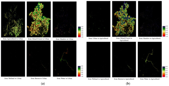
Figure 5.
Transition potential during 1989–1999 and 1999–2013. (a) Transition potential for agricultural land from 1989 to 1999. (b) Transition potential for urban land from 1999 to 2013.
Figure 5b verified an active change in the TPMs where agricultural and mixed-forest areas were transformed into urban areas. This result also responded to the 1999–2013 result for TPM indicated in Table 8. Particularly, the TPM of the mixed-forest area indicated in Figure 5b is more complex than that in Figure 5a. This result was affected by the similar types of roads seen in Figure 2. In other words, the development of the urban area was matched with the general urban development that is affected by roads.
4.3. Prediction Results and the Effectiveness of Local Regulation
As indicated in Table 9, the LUCC prediction for 2018 from the TPM obtained based on the 1989–1999 transition sub-model was named P-LULC1989–1999, the LUCC prediction for 2018 from the TPM obtained based on the 1999–2013 transition sub-model was denoted P-LULC1999–2013, and the LULC for the current year 2018 was denoted LULC2018. The differences in the LULCs were then compared.
Table 9.
Result of LULC predictions and differences: (a) LULC2018 (present); (b) P-LULC1989-1999 (prediction of LULC 2018 under condition where SCA is not enforced, (c) P-LULC1999-2013 (prediction of LULC 2018 under condition where TMDL is not enforced.
The results of examining the main LULC are as follows. Based on LULC2018 in Table 9 a, the urban, agricultural, mixed-forest, and meadow areas were calculated to cover 248.7 km2 (5.8%), 790.7 km2 (18.6%), 2607.4 km2 (61.2%), and 361.6 km2 (8.5%), respectively. Based on P-LULC1989–1999 in Table 9 b, the urban, agricultural, mixed-forest, and meadow areas were calculated at 146.9 km2 (3.4%), 1169.7 km2 (27.5%), 2595.3 km2 (60.9%), and 185.6 km2 (4.4%), respectively. LULC1999–2013 in Table 9 c suggests urban, agricultural, mixed-forest, and meadow areas of 417.9 km2 (9.8%), 852.4 km2 (20.0%), 2543.8 km2 (59.7%), and 202.8 km2 (4.8%), respectively.
Difference_1 in Table 9 describes the difference between LULC2018 and P-LULC1998–1999. The result of examining the main LULC in consideration of Difference_1 indicates that the difference in the urban, agricultural, and meadow areas was −101.8 km2, 379.0 km2, and −176.0 km2, respectively. This result also verifies a significant increase in the amount of agricultural land compared to that gained via urbanization. This result was obtained because agricultural land showed the greatest probability of change (Sum-Itself) in consideration of the TPM based on the 1999–2013 transition sub-model, as indicated in Table 8. It was assumed that this was a result of the SCA regulation, the first regulation examined in this study, as shown in Figure 3. Difference_2 in Table 9 shows the difference between LULC2018 and P-LULC1999–2013. The result of examining the main LULC in consideration of Difference_2 indicates that the area covered by urban, agricultural, mixed-forest, and meadow was 169.2 km2, 61.8 km2, −63.6 km2, and −158.8 km2, respectively. This result was derived because the urban, agricultural, mixed-forest, and meadow areas accounted for most of the probable change (Sum-Itself) if the TPM for the 1999–2013 transition sub-model in P-LULC1999–2013 is considered, as indicated in Table 8. This result is assumed to be a result of the TMDL regulation, the second regulation examined in this study, as shown in Figure 3. The LUCC can be visually observed in Figure 6. The result of LULC2018 (Figure 6a) shows that agriculture was mainly developed in the south-east of the studied basin. The result of P-LULC1989–1999 (Figure 6b) shows that this agricultural area expanded, with most changes observed near rivers. The result of LULC2018 also indicates that urbanization was concentrated in the western part of the study area as a result of the SCA regulation. Unlike this result, the result of LULC1999–2013 (Figure 6c) shows that areas lying adjacent to rivers and roads underwent equal amounts of urbanization.
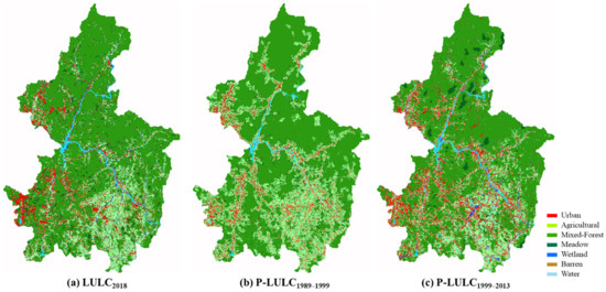
Figure 6.
Raster of the LULC prediction results: (a) LULC2018 (present); (b) P-LULC1989-1999 (prediction of LULC 2018 under condition where SCA is not enforced), (c) P-LULC1999-2013 (prediction of LULC 2018 under condition where TMDL is not enforced).
In a previous study of LULC regulation, Nixon and Newman [55] analyzed the effectiveness of the Agricultural Land Reserve (ALR) regulation for a study area in British Columbia; the study area’s southwestern region had colossal development pressure, which could affect the study area. This study evaluated that the policy successfully led to the conservation of agricultural areas and prevented urban expansion. Subiyanto and Fadilla [56] analyzed urban expansion in Indonesia and reported an increase in urban areas between 2005 and 2017, while farmland, grassland, and wetlands declined. Li [57] assessed regulations for farmland conservation in China. Although it could not provide direct evidence, the study reported that farmland increased during the study period, but forest area decreased. Zhang [58] analyzed the land use policy in Beijing from 1949 to 2009. To this end, the study divided the study period into three phases. In phases 1–2, the concept of basic urban planning and specialized agricultural land protection policies were established, and in phases 2–3, the basic plan for land use was mentioned to adjust the basic urban plan and it was reported that it was effective in the conservation of farmland in Beijing. Through the previous studies, it can be assumed that regulations can have a huge impact on LULC.
Generally, the LULC that exerts negative effects on water quality includes both urban and agricultural areas where human activities are concentrated. The results of the SCA and TMDL regulations analysis in this study and the aforementioned previous studies indicate that the SCA regulation brought about positive regulatory effects by limiting the increase in agricultural land to approximately 379 km2 and negative effects in an observed increase of approximately 102 km2 for the urban area. The TMDL regulations brought about positive regulatory effects by limiting the increase of urbanization to approximately 169.2 km2 and an increase in agricultural land to approximately 61.8 km2.
Table 10 shows the differences in the water pollutant loads based on the data indicated in Table 9. This data is used to identify changes in the amount of water pollution emitted according to the LUCC with local regulations applied. Table 10a shows the values that were obtained by subtracting the water pollutant loads in P-LULC1999–2013 from the water pollutant loads in P-LULC1989–1999. The sum of the water pollutants based on BOD, TN, and TP was calculated to be negative despite an increase in agricultural and mixed-forest areas. This result was obtained because the amount of water pollutant unit-loads emitted from the urban areas is 44–92 times greater than that released by other types of LU based on BOD, and is 8–18 times greater based on TN and 5–78 times as large in terms of TP. These differences in the water pollutant unit-loads indicate that the urban area is the main cause of water pollution compared to the other types of LULC. These results indicate that reducing the amount of water pollutants released will not occur unless LUCC is carried out over a certain scale despite the enhanced transformation of LULC to agricultural land.
Table 10.
Variation in the pollutant load difference: (a) BOD, TN and TP loads under condition where SCA is not enfoced; (b) BOD, TN and TP loads under condition where TMDL is not enforced.
Table 10b shows the result that is obtained by subtracting the water pollutant loads in P-LULC1999–2013 from the water pollutant loads in LULC2018. Unlike the results in Table 10a, this result indicates that the sum of the water pollutant loads based on BOD, TN, and TP is positive. This result verifies the positive effects of the TMDL regulation in terms of preserving the water quality under the increases in both urban and agricultural areas, as indicated in Table 9. In addition, the water pollutant unit-loads in the urban area are regarded as the main cause of the increase, as mentioned above. Particularly, Table 10b shows that the sum of water pollutant loads based on BOD, TN, and TP was similar to that observed in urban areas. This result might have been affected by a fluctuation in the LULC changes that did not include the urban area. However, the analysis suggests that the result was mainly affected by the fact that water pollutant loads generated by other types of LULCs had insignificant effects on the changes observed in terms of pollutant loading.
As a previous study of water quality change due to LUCC, Kalkidan et al. [59] reported a significant contribution to water pollution loads from urban areas and forests for deteriorating water quality. Nafi’Shehab et al. [60] analyzed the causes of water quality deterioration in the Bentong River in Malaysia and reported that urban and agricultural areas affect water quality deterioration and forests affect water quality improvement. Rajib et al. [61] examined future LUCC might affect water quality changes in South Dakota, U.S., where agricultural areas are dominant. As a result, forest, grassland, and high-input agricultural areas were transformed into urban and low-input agricultural areas, and the pollution load of nitrates and TP was reported to have decreased by 3–14%. As such, this study also showed that pollutant loads vary depending on LUCC and pollutant unit-loads. In particular, urban areas are the main source of pollutant load, which is absolute compared to other LULCs. In addition, this study found that even if LULC converted a large area to agricultural use, it could not have a positive effect on pollutant load unless a certain amount of LUCC occurs.
This result suggests that the method used to analyze the effects of local regulations based on the Ca-Markov model is an alternative tool that can be used to intuitively derive LUCC simulation results that reflect the tendencies of human activities. However, it is difficult to represent simultaneous human-social effects using the CA-Markov model. In this regard, simulating the effects that local regulations have in relation to human activities instead of simulating the effects that local regulations have on specific fields can result in generalization, as shown in the cases of the SCA and TMDL regulations. In other words, LUCC can occur rapidly or gradually over long periods according to changes in conditions such as policies implemented by the government or economic revitalization. For this reason, the tendencies of LUCC are unlikely to be generalized, and the demand for collecting LULC data with which to analyze such tendencies cannot be met. Thus, further studies will be conducted to develop a model that can reflect fluctuating conditions and analyze LUCC in consideration of more stereoscopic regulations.
5. Conclusions
This study aimed to examine the effects of local regulations that were implemented to protect the main water resources in South Korea. To this end, this study conducted LUCC simulation using the CA-Markov model without the application of the local regulations applied via the SCA and TMDL. The results of the simulation were then compared with practical LULC data to ascertain the effects of the local regulations. The results indicated that the area covered by agricultural land increased significantly when the SCA regulation was not applied while urbanization increased significantly when the TMDL regulation was not applied. Moreover, the result of examining the changes in water pollutant loading according to LUCC showed that an increase in agricultural land and a decrease in urbanization were observed when the SCA regulation was not applied and that the total amount of water pollutants in the basin decreased compared to the present LULC. In addition, it was found that the size of the urban areas increased compared to the current LULC and that the total amount of water pollutant loads increased when the TMDL regulations were not applied.
In other words, South Korea’s SCA regulation has both positive regulatory effects of the suppression of agricultural growth and negative regulatory effects of an increasing urban area, while the TMDL regulation has the positive regulatory effects of the suppression of urban growth and agricultural growth. In terms of pollutant load, urban areas are the main cause of pollutant load, which is absolute compared to other LULCs. It was also found that even if land use is concentrated and converted to agricultural, it could not have a positive effect on water pollution load unless there is a certain amount of LUCC.
However, LULC prediction using the CA-Markov model has technical limitations in that LUCC simulation is very difficult to be carried out under ever-changing conditions such as governmental policies and economic revitalization, and that human-social effects that occur simultaneously cannot be analyzed. In addition, this study could not reflect the actual water quality change mechanism in a river because the pollutant load was calculated using only pollutant unit-load. Nevertheless, using a methodology based on the CA-Markov model to analyze the effect of local regulations, as proposed in this study, is evaluated as being a better analysis tool for engineering rather than the socio-scientific fields. Therefore, the proposed methodology is a simpler, more intuitive, and efficient means of analyzing the effects of regulations and can predict the LU changes that reflect human activities well while exhibiting satisfactory prediction performance.
Funding
This research received no external funding.
Institutional Review Board Statement
Not applicable.
Informed Consent Statement
Not applicable.
Data Availability Statement
Not applicable.
Conflicts of Interest
The author declares no conflict of interest.
References
- Geist, H.J.; Lambin, E.F. Proximate causes and underlying driving forces of tropical deforestation. Bioscience 2002, 52, 143–150. [Google Scholar] [CrossRef]
- Ali, H. Land Use and Land Cover Change, Drivers and Its Impact: A Comparative Study from Kuhar Michael and Lenche Dima of Blue Nile and Awash Basins of Ethiopia. Ph.D. Thesis, Cornell University, New York, NY, USA, 2009. [Google Scholar]
- Singh, S.K.; Mustak, S.; Srivastava, P.K.; Szabó, S.; Islam, T. Predicting spatial and decadal LULC changes through cellular automata Markov chain models using earth observation datasets and geo-information. Environ. Process. 2015, 2, 61–78. [Google Scholar] [CrossRef]
- Francesch-Huidobro, M.; Dabrowski, M.; Tai, Y.; Chan, F.; Stead, D. Governance challenges of flood-prone delta cities: Integrating flood risk management and climate change in spatial planning. Prog. Plann. 2017, 114, 1–27. [Google Scholar] [CrossRef]
- Robi, M.A.; Abebe, A.; Pingale, S.M. Flood hazard mapping under a climate change scenario in a Ribb catchment of Blue Nile River basin, Ethiopia. Appl. Geomat. 2019, 11, 147–160. [Google Scholar] [CrossRef]
- Zampella, R.A.; Procopio, N.A.; Lathrop, R.G.; Dow, C.L. Relationship of Land-Use/Land-Cover Patterns and Surface-Water Quality in the Mullica River Basin. JAWRA 2007, 43, 594–604. [Google Scholar] [CrossRef]
- Meneses, B.M.; Reis, R.; Vale, M.J.; Saraiva, R. Land use and land cover changes in Zêzere watershed (Portugal)—Water quality implications. Sci. Total Environ. 2015, 527, 439–447. [Google Scholar] [CrossRef]
- Shi, P.; Zhang, Y.; Li, Z.; Li, P.; Xu, G. Influence of land use and land cover patterns on seasonal water quality at multi-spatial scales. Catena 2017, 151, 182–190. [Google Scholar] [CrossRef]
- Dezhkam, S.; Amiri, B.J.; Darvishsefat, A.A.; Sakieh, Y. Performance evaluation of land change simulation models using landscape metrics. Geocarto Int. 2017, 32, 655–677. [Google Scholar] [CrossRef]
- Hwang, J.H.; Park, S.H.; Song, C.M. A Study on an Integrated Water Quantity and Water Quality Evaluation Method for the Implementation of Integrated Water Resource Management Policies in the Republic of Korea. Water 2020, 12, 2346. [Google Scholar] [CrossRef]
- Hasan, S.; Shi, W.; Zhu, X.; Abbas, S.; Khan, H.U.A. Future Simulation of Land Use Changes in Rapidly Urbanizing South China Based on Land Change Modeler and Remote Sensing Data. Sustainability 2020, 12, 4350. [Google Scholar] [CrossRef]
- Hamad, R.; Balzter, H.; Kolo, K. Predicting Land Use/Land Cover Changes Using a CA-Markov Model under Two Different Scenarios. Sustainability 2018, 10, 3421. [Google Scholar] [CrossRef]
- Salem, M.; Tsurusaki, N.; Divigalpitiya, P. Analyzing the Driving Factors Causing Urban Expansion in the Peri-Urban Areas Using Logistic Regression: A Case Study of the Greater Cairo Region. Infrastructures 2019, 4, 4. [Google Scholar] [CrossRef]
- Ansari, A.; Golabi, M.H. Prediction of spatial land use changes based on LCM in a GIS environment for Desert Wetlands—A case study: Meighan Wetland, Iran. Int. Soil Water Conserv. Res. 2019, 7, 64–70. [Google Scholar] [CrossRef]
- EGIS: Environment Geographic Information Service. Available online: https://egis.me.go.kr (accessed on 5 November 2020).
- Ruben, G.B.; Zhang, K.; Dong, Z.; Jun, X. Analysis and Projection of Land-Use/Land-Cover Dynamics through Scenario-Based Simulations Using the CA-Markov Model: A Case Study in Guanting Reservoir Basin, China. Sustainability 2020, 12, 3747. [Google Scholar] [CrossRef]
- Omar, N.Q.; Ahamad, M.S.S.; Hussin, W.M.A.W.; Samat, N.; Ahmad, S.Z. Markov CA, Multi Regression, and Multiple Decision Making for Modeling Historical Changes in Kirkuk City, Iraq. J. Indian Soc. Remote Sens. 2013, 42, 165–178. [Google Scholar] [CrossRef]
- WAMIS: Water Management Information System, National Institute of Environmental Research. Available online: https://www.water.nier.go.kr (accessed on 7 November 2020).
- NTIC: National Transport Information Center. Available online: https://intl.its.go.kr/en/02_05_09 (accessed on 11 November 2020).
- Arnold, J.G.; Allen, P.M.; Bernhardt, G. A comprehensive surface-groundwater flow model. J. Hydrol. 1993, 142, 47–69. [Google Scholar] [CrossRef]
- Young, R.A.; Onstad, C.A.; Bosch, D.D.; Anderson, W.P. AGNPS: A Nonpoint Source Pollution Model for Evaluating Agricultural Watersheds. J. Soil Water Conserv. 1989, 44, 168–173. Available online: https://www.jswconline.org/content/44/2/168 (accessed on 1 March 2021).
- Rossman, L.A. Storm Water Management Model User’s Manual, 5th ed.; Water Supply and Water Resources Division National Risk Management Research Laboratory, Office of Research and Development: Cincinnati, OH, USA, 2010; p. 276.
- Aisha, M.S. Evaluation of SWAT Model Applicability for Water Impairment Identification and TMDL Analysis. Ph.D. Thesis, University of Maryland, College Park, MD, USA, 30 October 2007. [Google Scholar]
- EPA. Storm Water Management for Industrial Activities. Pollution Prevention Plans and Best Management Practices; Office of Water-EPA: Washington, DC, USA, 1993.
- Wanielista, M.P.; Yousef, Y.A.; McLellon, W.M. Nonpoint source effects on water quality. Water Pollut. Control Fed. 1977, 49, 441–451. Available online: https://www.jstor.org/stable/25039287 (accessed on 12 February 2021).
- NIER. Technical Guidelines for TMDLs; Korean Literature; National Institute Environment Research: Incheon, Korea, 2014.
- Parsa, V.A.; Yavari, A.; Nejadi, A. Spatio-temporal analysis of land use/land cover pattern changes in Arasbaran Biosphere Reserve: Iran. Model. Earth Syst. Environ. 2016, 2, 1–13. [Google Scholar] [CrossRef]
- Liu, Y.; Dai, L.; Xiong, H. Simulation of urban expansion patterns by integrating auto-logistic regression, Markov chain and cellular automata models. J. Environ. Plan. Manag. 2015, 58, 1113–1136. [Google Scholar] [CrossRef]
- Hsu, L.C. Applying the Grey prediction model to the global integrated circuit industry. Technol. Forecast. Soc. Chang. 2003, 70, 563–574. [Google Scholar] [CrossRef]
- Weng, Q. Land use change analysis in the Zhujiang Delta of China using satellite remote sensing, GIS and stochastic modelling. J. Environ. Manag. 2002, 64, 273–284. [Google Scholar] [CrossRef] [PubMed]
- Mishra, V.N.; Rai, P.K.; Mohan, K. Prediction of land use changes based on land change modeler (LCM) using remote sensing: A case study of Muzaffarpur (Bihar), India. J. Geogr. Inst. Jovan Cvijic SASA 2014, 64, 111–127. [Google Scholar] [CrossRef]
- Murugesan, S.; Zhang, J.; Vittal, V. Finite state Markov chain model for wind generation forecast: A data-driven spatiotemporal approach. In Proceedings of the 2012 IEEE PES Innovative Smart Grid Technologies (ISGT), Washington, DC, USA, 16–20 January 2012; pp. 1–8. [Google Scholar] [CrossRef]
- Kumar, S.; Radhakrishnan, N.; Mathew, S. Land use change modelling using a Markov model and remote sensing. Geomat. Nat. Hazards Risk 2014, 5, 145–156. [Google Scholar] [CrossRef]
- Behera, M.D.; Borate, S.N.; Panda, S.N.; Behera, P.R.; Roy, P.S. Modelling and analyzing the watershed dynamics using Cellular Automata (CA)-Markov model—A geo-information based approach. J. Earth Syst. Sci. 2012, 121, 1011–1024. [Google Scholar] [CrossRef]
- Khawaldah, H.A. A Prediction of Future Land Use/Land Cover in Amman Area Using GIS-Based Markov Model and Remote Sensing. J. Geogr. Inf. Syst. 2016, 8, 412–427. [Google Scholar] [CrossRef]
- Faichia, C.; Tong, Z.; Zhang, J.; Liu, X.; Kazuva, E.; Ullah, K.; Al-Shaibah, B. Using RS Data-Based CA-Markov Model for Dynamic Simulation of Historical and Future LUCC in Vientiane, Laos. Sustainability 2020, 12, 8410. [Google Scholar] [CrossRef]
- Subedi, P.; Subedi, K.; Thapa, B. Application of a Hybrid Cellular Automaton-Markov (CA-Markov) Model in Land-Use Change Prediction: A Case Study of Saddle Creek Drainage Basin, Florida. Appl. Ecol. Environ. Sci. 2013, 1, 126–132. [Google Scholar] [CrossRef]
- Ye, B.; Bai, Z. Simulating land use/cover changes of Nenjiang County based on CA-Markov model. Comput. Technol. Agric. 2008, 1, 321–329. [Google Scholar] [CrossRef]
- Reddy, C.S.; Singh, S.; Dadhwal, V.K.; Jha, C.S.; Rao, N.R.; Diwakar, P.G. Predictive modelling of the spatial pattern of past and future forest cover changes in India. J. Earth Syst. Sci. 2017, 126. [Google Scholar] [CrossRef]
- Tajbakhsh, S.M.; Memarian, H.; Moradi, K.; Aghakhani Afshar, A.H. Performance comparison of land change modeling techniques for land use projection of arid watersheds. Glob. J. Environ. Sci. Manag. 2018, 4, 263–280. [Google Scholar] [CrossRef]
- Clark Labs. TerrSet Geospatial Monitoring and Modeling Software. Available online: https://clarklabs.org/terrset/ (accessed on 3 July 2020).
- Eastman, J.R. Idrisi Taiga Manual; Clark Lab, Clark University: Worcester, MA, USA, 2009. [Google Scholar]
- Eastman, J.R. Idrisi TerrSet 18.00; Clark University: Worcester, MA, USA, 2014. [Google Scholar]
- Eastman, J.R.; Crema, S.C.; Rush, H.R.; Zhang, K. A weighted normalized likelihood procedure for empirical land change modeling. Model. Earth Syst. Environ. 2019, 5, 985–996. [Google Scholar] [CrossRef]
- Landis, J.R.; Koch, G.G. The Measurement of Observer Agreement for Categorical Data. Biometrics 1977, 33, 159–174. [Google Scholar] [CrossRef]
- Song, C.M. Hydrological Image Building Using Curve Number and Prediction and Evaluation of Runoff through Convolution Neural Network. Water 2020, 12, 2292. [Google Scholar] [CrossRef]
- Kim, D.Y.; Song, C.M. Developing a Discharge Estimation Model for Ungauged Watershed Using CNN and Hydrological Image. Water 2020, 12, 3534. [Google Scholar] [CrossRef]
- Alqurashi, A.; Kumar, L. Investigating the use of remote sensing and GIS techniques to detect land use and land cover change: A review. Adv. Remote Sens. 2013, 2, 193–204. [Google Scholar] [CrossRef]
- E Silva, L.P.; Xavier, A.P.C.; da Silva, R.M.; Santos, C.A.G. Modeling land cover change based on an artificial neural network for a semiarid river basin in northeastern Brazil. Glob. Ecol. Conserv. 2020, 21, e00811. [Google Scholar] [CrossRef]
- Pérez-Vega, A.; Mas, J.F.; Ligmann-Zielinska, A. Comparing two approaches to land use/cover change modeling and their implications for the assessment of biodiversity loss in a deciduous tropical forest. Environ. Model. Softw. 2012, 29, 11–23. [Google Scholar] [CrossRef]
- Oñate-Valdivieso, F.; Bosque Sendra, J. Application of GIS and remote sensing techniques in generation of land use scenarios for hydrological modeling. J. Hydrol. 2010, 395, 256–263. [Google Scholar] [CrossRef]
- Xiao, J.; Shen, Y.; Ge, J.; Tateishi, R.; Tang, C.; Liang, Y.; Huang, Z. Evaluating urban expansion and land use change in Shijiazhuang, China, by using GIS and remote sensing. Landsc. Urban Plan. 2006, 75, 69–80. [Google Scholar] [CrossRef]
- Hassan, Z.; Shabbir, R.; Ahmad, S.S.; Malik, A.H.; Aziz, N.; Butt, A.; Erum, S. Dynamics of land use and land cover change (LULCC) using geospatial techniques: A case study of Islamabad Pakistan. SpringerPlus 2016, 5, 1–11. [Google Scholar] [CrossRef] [PubMed]
- Kogo, B.K.; Kumar, L.; Koech, R. Analysis of spatio-temporal dynamics of land use and cover changes in Western Kenya. Geocarto Int. 2021, 36, 376–391. [Google Scholar] [CrossRef]
- Nixon, D.V.; Newman, L. The efficacy and politics of farmland preservation through land use regulation: Changes in southwest British Columbia’s Agricultural Land Reserve. Land Use Policy 2016, 59, 227–240. [Google Scholar] [CrossRef]
- Subiyanto, S.; Fadilla, L. Monitoring land use change and urban sprawl based on spatial structure to prioritize specific regulations in Semarang, Indonesia. IOP Conf. Ser. Earth Environ. Sci. 2018, 179, 012029. [Google Scholar] [CrossRef]
- Li, M. The effect of land use regulations on farmland protection and non-agricultural land conversions in China. Aust. J. Agric. Resour. Econ. 2019, 63, 643–667. [Google Scholar] [CrossRef]
- Zhang, J. Historical changes in the land use regulation policy system in Beijing since 1949. J. Appl. Sci. 2012, 12, 2202–2214. [Google Scholar] [CrossRef]
- Kalkidan, A.; Hailu, W.; Mekuria, A. Assessing the impact of watershed land use on Kebena river water quality in Addis Ababa, Ethiopia. Environ. Syst. Res. 2021, 10. [Google Scholar] [CrossRef]
- Nafi’Shehab, Z.; Jamil, N.R.; Aris, A.Z.; Shafie, N.S. Spatial variation impact of landscape patterns and land use on water quality across an urbanized watershed in Bentong, Malaysia. Ecol. Indic. 2021, 122, 107254. [Google Scholar] [CrossRef]
- Rajib, M.A.; Ahiablame, L.; Paul, M. Modeling the effects of future land use change on water quality under multiple scenarios: A case study of low-input agriculture with hay/pasture production. Sustain. Water Qual. Ecol. 2016, 8, 50–66. [Google Scholar] [CrossRef]


Publisher’s Note: MDPI stays neutral with regard to jurisdictional claims in published maps and institutional affiliations. |
© 2021 by the author. Licensee MDPI, Basel, Switzerland. This article is an open access article distributed under the terms and conditions of the Creative Commons Attribution (CC BY) license (https://creativecommons.org/licenses/by/4.0/).