
Flood4castRTF: A Real-Time Urban Flood Forecasting Model

 , , ,
, , ,
Abstract
1. Introduction
1.1. Urban Flood Modelling
1.2. Real-Time Flood Forecasting
1.3. Improved Flood Modelling Approach
1.4. Novelty
- Integrated modelling remains possible at this scale, incorporating all relevant flow interactions in urban and rural catchments.
- An optimal balance is offered between model accuracy, model input accuracy, output accuracy and invested time for model build-up and simulations.
- Minimal data needs and automatic model build-up, as the approach does not require detailed data, for example on sewer elements, manholes, or surface run-off structures.
- The fast engine offers the opportunity to perform real-time simulations for large areas, and in the future even for real-time scenario simulations.
2. Materials and Methods
2.1. Model Concept
2.1.1. Surface Module: General Workflow
2.1.2. Surface Module: Stream Burning
2.1.3. Surface Module: Subgrid Approach
- A detailed water level–storage relationship per model cell also benefits these simplified approaches, especially for coarser grid cells that typically contain large topographic variations and therefore often are only partly flooded.
- The calculation of representative cross-sectional areas and hydraulic radii are facilitated by the detailed terrain data, as these can be processed to representative terrain profiles in-between two cell centres.
- A connectivity analysis at a variety of depths teaches how model cell sides are connected in different states of flooding. This way, cell internal throughflow can be blocked or limited when physical blockages occur in the terrain.
- Water level
- Storage volume
- Hydraulic radius and cross-sectional area (in 4 directions)
- Connectivity coefficients between each model cell side (12 combinations)
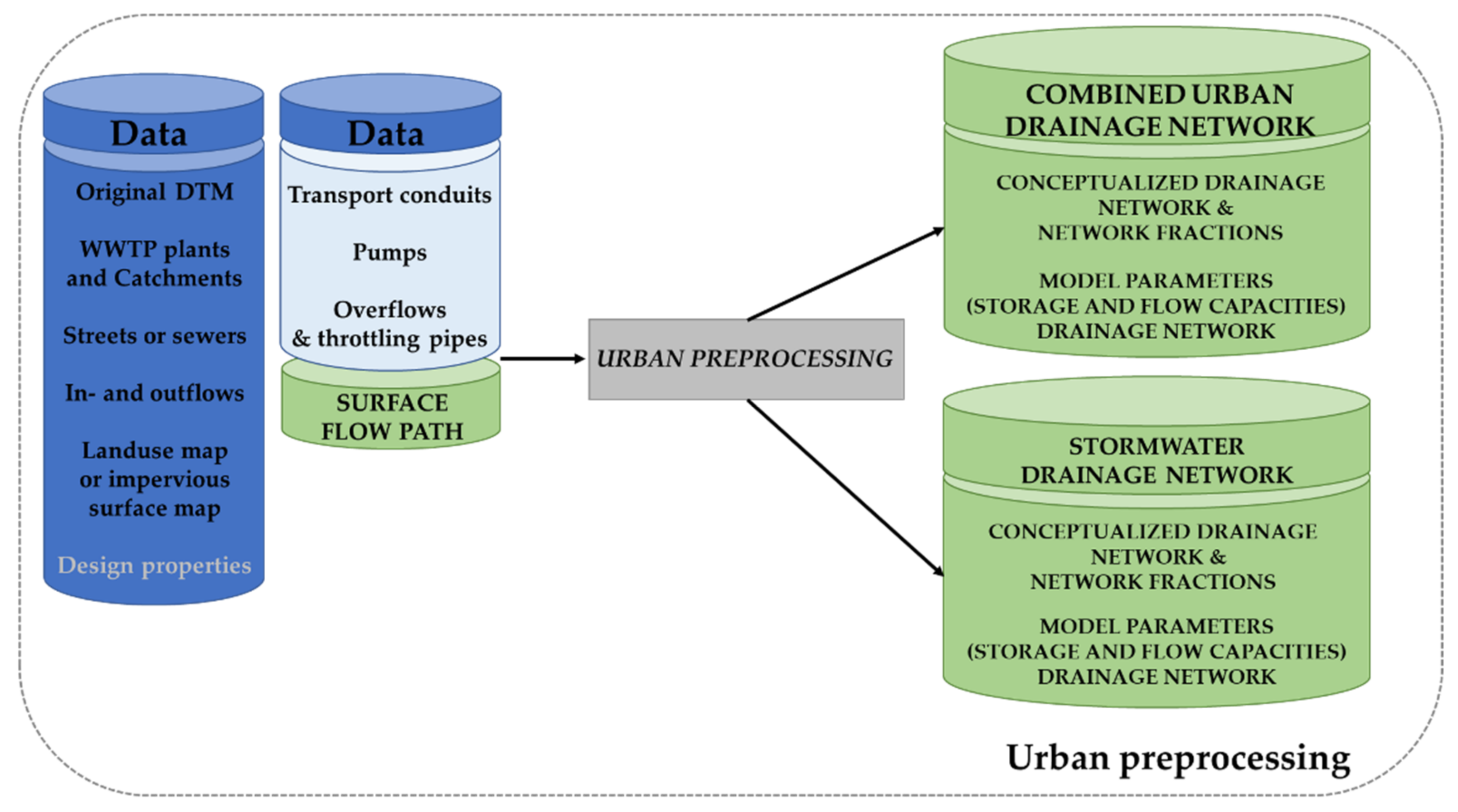
2.1.4. Urban Drainage Module: Sewer and Stormwater Network Conceptualisation
2.2. Case Study and Model Build-Up
2.2.1. Overview of Needed Data
- ○
- DTM data (the resolution of the terrain model determines the resolution of the flood maps);
- ○
- Information on the approximate location of the main stream network.
- ○
- Sewer network or street network;
- ○
- Land use map or impervious surface map;
- ○
- Location of urban structures like pumps, wastewater treatment plants, overflows, throttling locations and interactions with the surface layer.
2.2.2. Description Pilot Case
2.2.3. Surface Data
2.2.4. Urban Drainage Data
2.2.5. Rainfall Data and Climate Scenarios
2.2.6. Post-Processing
3. Results and Discussion
3.1. General
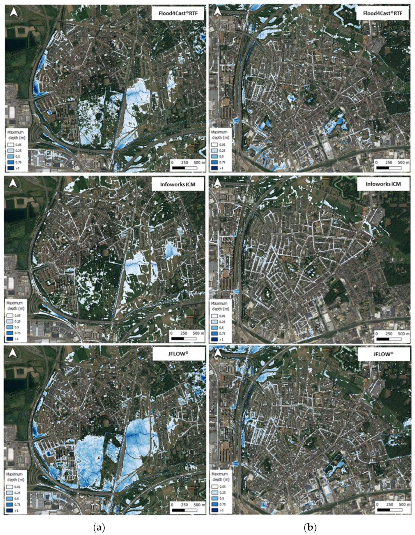
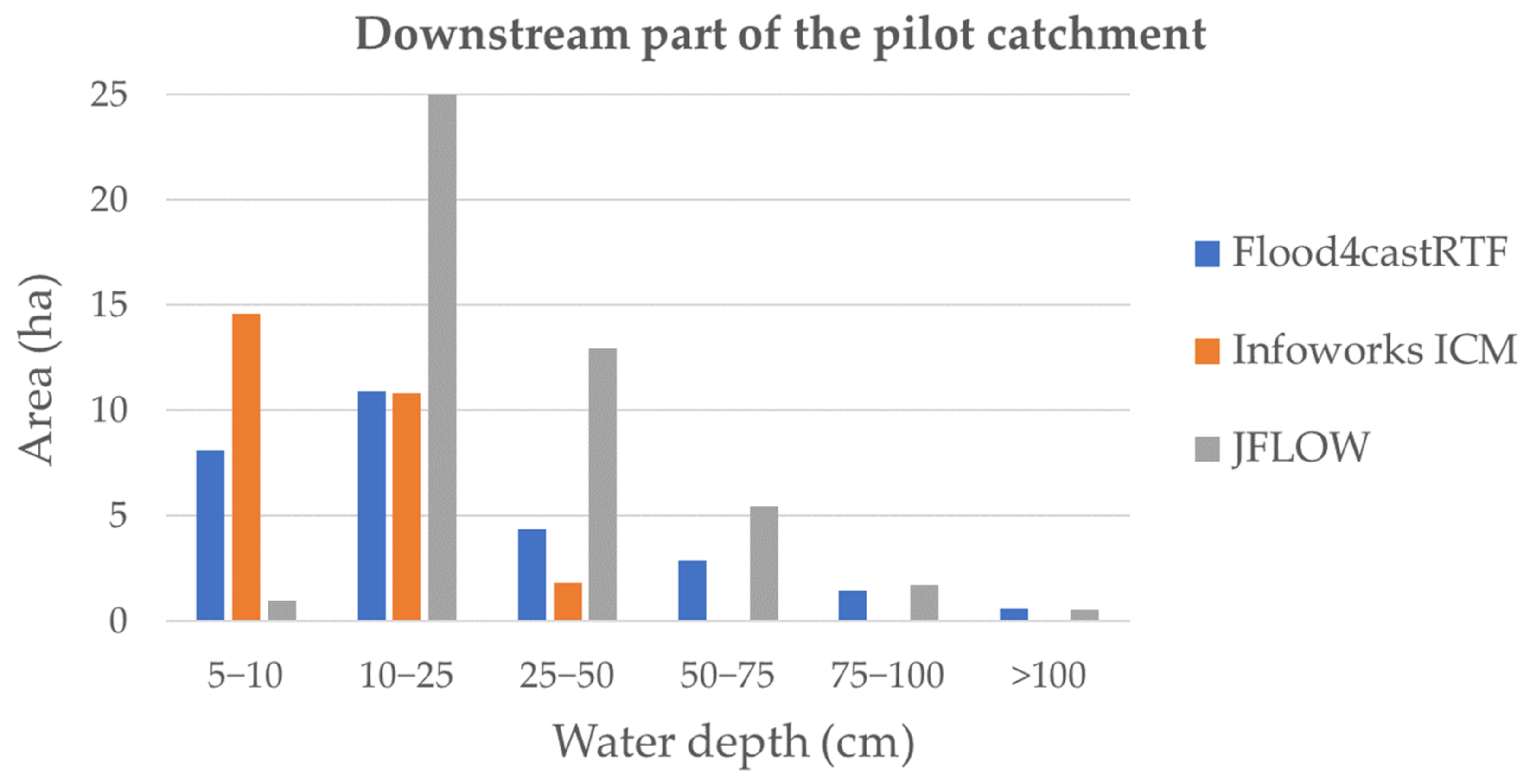
3.2. Flood Maps
3.3. Climate Change Scenario
3.4. Performance
3.4.1. Model Build-Up
3.4.2. Run-Time
3.4.3. Post-Processing
3.5. On the Use of the MANNING Equation
3.6. Applicability in Data-Scarce Areas
4. Conclusions
Author Contributions
Funding
Institutional Review Board Statement
Informed Consent Statement
Data Availability Statement
Conflicts of Interest
References
- Teng, J.; Jakeman, A.; Vaze, J.; Croke, B.F.W.; Dutta, D.; Kim, S. Flood inundation modelling: A review of methods, recent advances and uncertainty analysis. Environ. Model. Softw. 2017, 90, 201–216. [Google Scholar] [CrossRef]
- Bulti, D.T.; Abebe, B.G. A review of flood modeling methods for urban pluvial flood application. Model. Earth Syst. Environ. 2020, 6, 1293–1302. [Google Scholar] [CrossRef]
- Salvadore, E.; Bronders, J.; Batelaan, O. Hydrological modelling of urbanized catchments: A review and future directions. J. Hydrol. 2015, 529, 62–81. [Google Scholar] [CrossRef]
- Fatichi, S.; Vivoni, E.R.; Ogden, F.L.; Ivanov, V.Y.; Mirus, B.; Gochis, D.; Downer, C.W.; Camporese, M.; Davison, J.H.; Ebel, B.; et al. An overview of current applications, challenges, and future trends in distributed process-based models in hydrology. J. Hydrol. 2016, 537, 45–60. [Google Scholar] [CrossRef]
- Vivoni, E.R.; Mascaro, G.; Mniszewski, S.; Fasel, P.; Springer, E.P.; Ivanov, V.Y.; Bras, R.L. Real-world hydrologic assessment of a fully-distributed hydrological model in a parallel computing environment. J. Hydrol. 2011, 409, 483–496. [Google Scholar] [CrossRef]
- Costabile, P.; Costanzo, C.; De Lorenzo, G.; Macchione, F. Is local flood hazard assessment in urban areas significantly influenced by the physical complexity of the hydrodynamic inundation model? J. Hydrol. 2020, 580, 124231. [Google Scholar] [CrossRef]
- Arrighi, C.; Pregnolato, M.; Dawson, R.J.; Castelli, F. Preparedness against mobility disruption by floods. Sci. Total Environ. 2019, 654, 1010–1022. [Google Scholar] [CrossRef]
- Beven, K. Prophecy, reality and uncertainty in distributed hydrological modelling. Adv. Water Resour. 1993, 16, 41–51. [Google Scholar] [CrossRef]
- Van Dijk, E.; Van Der Meulen, J.; Kluck, J.; Straatman, J.H.M. Comparing modelling techniques for analysing urban pluvial flooding. Water Sci. Technol. 2013, 69, 305–311. [Google Scholar] [CrossRef]
- Cristiano, E.; Veldhuis, M.-C.T.; Van De Giesen, N. Spatial and temporal variability of rainfall and their effects on hydrological response in urban areas—A review. Hydrol. Earth Syst. Sci. 2017, 21, 3859–3878. [Google Scholar] [CrossRef]
- Hoch, J.M.; Van Beek, R.; Winsemius, H.C.; Bierkens, M.F. Benchmarking flexible meshes and regular grids for large-scale fluvial inundation modelling. Adv. Water Resour. 2018, 121, 350–360. [Google Scholar] [CrossRef]
- Ferraro, D.; Costabile, P.; Costanzo, C.; Petaccia, G.; Macchione, F. A spectral analysis approach for the a priori generation of computational grids in the 2-D hydrodynamic-based runoff simulations at a basin scale. J. Hydrol. 2020, 582, 124508. [Google Scholar] [CrossRef]
- Innovyze. InfoWorks ICM Product Page. Available online: https://www.innovyze.com/en-us/products/infoworks-icm (accessed on 21 January 2021).
- Casulli, V. A high-resolution wetting and drying algorithm for free-surface hydrodynamics. Int. J. Numer. Methods Fluids 2009, 60, 391–408. [Google Scholar] [CrossRef]
- Jamali, B.; Löwe, R.; Bach, P.M.; Urich, C.; Arnbjerg-Nielsen, K.; Deletic, A. A rapid urban flood inundation and damage assessment model. J. Hydrol. 2018, 564, 1085–1098. [Google Scholar] [CrossRef]
- Burger, G.; Sitzenfrei, R.; Kleidorfer, M.; Rauch, W. Parallel flow routing in SWMM 5. Environ. Model. Softw. 2014, 53, 27–34. [Google Scholar] [CrossRef]
- Kalyanapu, A.J.; Shankar, S.; Pardyjak, E.R.; Judi, D.R.; Burian, S.J. Assessment of GPU computational enhancement to a 2D flood model. Environ. Model. Softw. 2011, 26, 1009–1016. [Google Scholar] [CrossRef]
- Bates, P.D.; Horritt, M.S.; Fewtrell, T.J. A simple inertial formulation of the shallow water equations for efficient two-dimensional flood inundation modelling. J. Hydrol. 2010, 387, 33–45. [Google Scholar] [CrossRef]
- Guidolin, M.; Chen, A.S.; Ghimire, B.; Keedwell, E.C.; Djordjević, S.; Savić, D.A. A weighted cellular automata 2D inundation model for rapid flood analysis. Environ. Model. Softw. 2016, 84, 378–394. [Google Scholar] [CrossRef]
- Wolfs, V.; Willems, P. A data driven approach using Takagi–Sugeno models for computationally efficient lumped floodplain modelling. J. Hydrol. 2013, 503, 222–232. [Google Scholar] [CrossRef]
- Li, X.; Willems, P. A Hybrid Model for Fast and Probabilistic Urban Pluvial Flood Prediction. Water Resour. Res. 2020, 56, e2019WR025128. [Google Scholar] [CrossRef]
- Courant, R.; Friedrichs, K.; Lewy, H. Über die partiellen Differenzengleichungen der mathematischen Physik. Math. Ann. 1928, 100, 32–74. [Google Scholar] [CrossRef]
- Lindsay, J.B. Efficient hybrid breaching-filling sink removal methods for flow path enforcement in digital elevation models. Hydrol. Process. 2015, 30, 846–857. [Google Scholar] [CrossRef]
- Bates, P.D. Development and testing of a sub-grid scale model for moving-boundary hydrodynamic problems in shal-low water. Hydrol. Process. 2000, 14, 2073–2088. [Google Scholar] [CrossRef]
- Yu, D.; Lane, S.N. Urban fluvial flood modelling using a two-dimensional diffusion-wave treatment, part 2: Development of a sub-grid-scale treatment. Hydrol. Process. 2005, 20, 1567–1583. [Google Scholar] [CrossRef]
- Cea, L.; Vázquez-Cendon, M.E. Unstructured finite volume discretization of two-dimensional depth-averaged shallow water equations with porosity. Int. J. Numer. Methods Fluids 2009, 63, 903–930. [Google Scholar] [CrossRef]
- Stelling, G.S. Quadtree flood simulations with sub-grid digital elevation models. Proc. Inst. Civ. Eng. Water Manag. 2012, 165, 567–580. [Google Scholar] [CrossRef]
- Volp, N.D.; Van Prooijen, B.C.; Stelling, G.S. A finite volume approach for shallow water flow accounting for high-resolution bathymetry and roughness data. Water Resour. Res. 2013, 49, 4126–4135. [Google Scholar] [CrossRef]
- Geopunt Vlaanderen. Available online: https://www.geopunt.be (accessed on 29 April 2021).
- Vaes, G. The Influence of Rainfall and Model Simplification on the Design of Combined Sewer Systems. Ph.D. Thesis, Katholieke Universiteit Leuven, Leuven, Belgium, 1999. [Google Scholar]
- Brouwers, J.; Peeters, B.; Van Steertegem, M.; Van Lipzig, N.; Wouters, H.; Beullens, J.; Demuzere, M.; Willems, P.; De Ridder, K.; Maiheu, B.; et al. MIRA Climate Report 2015, about Observed and Future Climate Changes in Flanders and Belgium; Flanders Environment Agency: Aalst, Belgium, 2015. [Google Scholar] [CrossRef]
- Flemish Environmental Agency. Calculation of Fluvial Flood Maps for Flanders. 2018. Available online: https://www.vmm.be/publicaties/aanmaak-van-een-afstromingsgevoelige-kaart-voor-vlaanderen# (accessed on 29 April 2021). (In Dutch).
- JBA Consulting. JFLOW Product Page. Available online: https://www.jbaconsulting.com/knowledge-hub/jflow/ (accessed on 21 January 2021).
- Flemish Environmental Agency. Climate Portal Flanders. Available online: https://klimaat.vmm.be/nl (accessed on 21 January 2021). (In Dutch).
- Wang, Y.; Chen, A.S.; Fu, G.; Djordjević, S.; Zhang, C.; Savić, D.A. An integrated framework for high-resolution urban flood modelling considering multiple information sources and urban features. Environ. Model. Softw. 2018, 107, 85–95. [Google Scholar] [CrossRef]
- Chang, T.-J.; Wang, C.-H.; Chen, A.S. A novel approach to model dynamic flow interactions between storm sewer system and overland surface for different land covers in urban areas. J. Hydrol. 2015, 524, 662–679. [Google Scholar] [CrossRef]
- De Almeida, G.A.M.; Bates, P.; Ozdemir, H. Modelling urban floods at submetre resolution: Challenges or opportunities for flood risk management? J. Flood Risk Manag. 2016, 11, S855–S865. [Google Scholar] [CrossRef]
- Ozdemir, H.; Sampson, C.C.; De Almeida, G.A.M.; Bates, P.D. Evaluating scale and roughness effects in urban flood modelling using terrestrial LIDAR data. Hydrol. Earth Syst. Sci. 2013, 17, 4015–4030. [Google Scholar] [CrossRef]
- Farr, T.G.; Rosen, P.A.; Caro, E.; Crippen, R.; Duren, R.; Hensley, S.; Kobrick, M.; Paller, M.; Rodriguez, E.; Roth, L.; et al. The Shuttle Radar Topography Mission. Rev. Geophys. 2007, 45. [Google Scholar] [CrossRef]
- Gong, P.; Wang, J.; Yu, L.; Zhao, Y.; Zhao, Y.; Liang, L.; Niu, Z.; Huang, X.; Fu, H.; Liu, S.; et al. Finer resolution observation and monitoring of global land cover: First mapping results with Landsat TM and ETM+ data. Int. J. Remote Sens. 2012, 34, 2607–2654. [Google Scholar] [CrossRef]


| Observation | |||
|---|---|---|---|
| Positive | Negative | ||
| Simulation | Positive | True positive (TP) | False positive (FP) |
| Negative | False Negative (FN) | True Negative | |
| JFLOW | Flood4castRTF | ||||
|---|---|---|---|---|---|
| flooded | not flooded | TPR | PPV | ||
| Ekeren | flooded | 19.5 | 27.5 | 0.42 | 0.69 |
| not flooded | 8.9 | ||||
| Infoworks ICM | 0.37 | 0.63 | |||
| Merksem | flooded | 45.0 | 31.9 | 0.59 | 0.58 |
| not flooded | 33.2 | ||||
| Infoworks ICM | 0.53 | 0.60 | |||
| Infoworks ICM | Flood4castRTF | ||||
| flooded | not flooded | TPR | PPV | ||
| Ekeren | flooded | 11.6 | 15.8 | 0.42 | 0.41 |
| not flooded | 16.8 | ||||
| JFLOW | 0.63 | 0.37 | |||
| Merksem | flooded | 34.0 | 34.8 | 0.49 | 0.44 |
| not flooded | 44.2 | ||||
| JFLOW | 0.60 | 0.53 | |||
| Process | Specification | Time | Repetition |
|---|---|---|---|
| General GIS pre-processing | Model mask, DTM, imperviousness | 1 min | 1 |
| Surface layer pre-processing | Stream burning | 5 min | 1 (1) |
| Local drain direction (LDD) | 6.3 h | 1 (1) | |
| Subgrids | 10 h | 1 (1) | |
| Urban drainage pre-processing | Cell-to-cell runoff fractions and objects | 32 min | 1 |
| Optimisation of parameters | 32 min | O(10) (2) |
| Process | Specification | Time | Repetition |
|---|---|---|---|
| Run-time | Initialisation | 19 s. | 1 (per scenario) |
| Rain module | 2 s. | ||
| Surface module | 126 s. | ||
| Urban drainage module | 21 s. | ||
| Output module | 23 s. | ||
| Total | 191 s. |
Publisher’s Note: MDPI stays neutral with regard to jurisdictional claims in published maps and institutional affiliations. |
© 2021 by the authors. Licensee MDPI, Basel, Switzerland. This article is an open access article distributed under the terms and conditions of the Creative Commons Attribution (CC BY) license (https://creativecommons.org/licenses/by/4.0/).
Share and Cite
Craninx, M.; Hilgersom, K.; Dams, J.; Vaes, G.; Danckaert, T.; Bronders, J. Flood4castRTF: A Real-Time Urban Flood Forecasting Model. Sustainability 2021, 13, 5651. https://doi.org/10.3390/su13105651
Craninx M, Hilgersom K, Dams J, Vaes G, Danckaert T, Bronders J. Flood4castRTF: A Real-Time Urban Flood Forecasting Model. Sustainability. 2021; 13(10):5651. https://doi.org/10.3390/su13105651
Chicago/Turabian StyleCraninx, Michel, Koen Hilgersom, Jef Dams, Guido Vaes, Thomas Danckaert, and Jan Bronders. 2021. "Flood4castRTF: A Real-Time Urban Flood Forecasting Model" Sustainability 13, no. 10: 5651. https://doi.org/10.3390/su13105651
APA StyleCraninx, M., Hilgersom, K., Dams, J., Vaes, G., Danckaert, T., & Bronders, J. (2021). Flood4castRTF: A Real-Time Urban Flood Forecasting Model. Sustainability, 13(10), 5651. https://doi.org/10.3390/su13105651