Improving the Performance of Single-Intersection Urban Traffic Networks Based on a Model Predictive Controller

Abstract

The use of a Model Predictive Controller (MPC) in an urban traffic network allows for controlling the infrastructure of a traffic network and errors in its operations. In this research, a novel, stable predictive controller for urban traffic is proposed and state-space dynamics are used to estimate the number of vehicles at an isolated intersection and the length of its queue. This is a novel control strategy based on the type of traffic light and on the duration of the green-light phase and aims to achieve an optimal balance at intersections. This balance should be adaptable to the unchanging behavior of time and to the randomness of traffic situations. The proposed method reduces traffic volumes and the number of crashes involving cars by controlling traffic on an urban road using model predictive control. A single intersection in Tehran, the capital city of Iran, was considered in our study to control traffic signal timing, and model predictive control was used to reduce traffic. A model of traffic systems was extracted at the intersection, and the state-space parameters of the intersection were designed using the model predictive controller to control traffic signals based on the length of the vehicle queue and on the number of inbound and outbound vehicles, which were used as inputs. This process demonstrates that this method is able to reduce traffic volumes at each leg of an intersection and to optimize flow in a road network compared to the fixed-time method.

1. Introduction

Due to population growth, economics, social and cultural changes, and immigration [1,2], communities are rapidly developing and changing. With this urbanization, the number of vehicles has increased, especially in large cities, and problems involving these vehicles have arisen. Although it is very costly to build new roads every year, traffic is still an ongoing problem and causes congestion, especially at rush hour. Traffic peaks wordwide have become some of the biggest problems in urban areas, increasing traffic flow and imposing high costs for society at various levels. The importance of traffic control has increased due to its close relationship with issues such as air pollution, fuel consumption, and security issues, and traffic control systems are being used worldwide to improve the impact of traffic flow [3,4,5]. According to Chedjou et al. [6], this problem has become serious in developing countries in Asia because the vehicle ownership ratio and freight traffic volume have increased.

In the work by Papageorgiou and Araghi et al. [7,8], traffic lights at intersections were considered one of the most effective means of controlling urban traffic. Traffic-reduction and better-optimized control methods can reduce travel times along a route and vehicle queues. Zhao et al. [9] suggested that traffic can be controlled using fixed-time and smart methods. According to the work by Zhao et al. [10], the time constant of an intersection control method was either local or coordinated and the implementation of their method was set as offline for some hours of the day for optimization. Different dynamical models in traffic control have also been discussed. Silva et al. [11] established a multi-objective signal-timing optimization model to optimize average vehicle delay, slow traffic delay, vehicle stopping times, and traffic capacity. The experimental results showed that the model optimized traffic by reducing vehicle delays, slow traffic delays, stopping times at an intersection, and increasing traffic capacity.

Ye et al. [12] presented a novel traffic device (Lan-Pro) that avoids vehicles stopping at junctions in low-traffic conditions. The results show that the proposal may ensure non-stop crossing of intersections when traffic volume is expected to be high, and their primary goal is to handle low-traffic conditions.

Stochastic model predictive control for signal coordination and control of transactions in urban pedestrian networks was presented in the work by Shihuang et al. [13]. One important feature in stochastic model predictive control (MPC) is that uncertain traffic demands and stochastic disturbances are considered. This is a random value model with odds limits used in a random targeted performance. The purpose is to model uncertainties and to prevent queuing at traffic networks to minimize queue length and green-light duration fluctuations between the two control stages. Finally, a hybrid smart algorithm (neural networks in the genetic algorithm) was proposed to solve random model predictive control (MPC). Thus far, traffic control processes have been based on classic control methods, which use statistical methods. However, due to the complex traffic control structure, an adequate response cannot be obtained using these methods. For this reason, with the development of smart methods, including artificial intelligence, fuzzy logic, neural networks, multiprocessor systems, etc., they can help solve and improve urban management problems.

Zhao et al. [9] used a neural network with a training set. Brian et al. [14] used an intersectional neural network and intersection to create a smart agent varying the green-light duration of each cycle based on the information presented to improve its accuracy. Fiore et al. [15] presented a genetic algorithm to optimize traffic signals for saturated conditions. Various optimization strategies were used to provide minimal delay and were evaluated to maximize power at various intersections. Lin et al. [16] presented a model for traffic queue using the average vehicle wait time. Push control is an optimal control method based on the theory of transverse horizons. Including smart control methods, a pre-control method was developed. In Li et al. [17], model predictive control was used to control and coordinate urban transport networks; optimization of the pre-control nonlinear model requires long computational times due to the nonlinearity of the problem of optimizing combined logical programming.

Following these developments, new dynamic multipurpose optimization systems for the predictive control of existing network signals have been designed and presented. Two network models have been proposed. A network signal prediction control algorithm has been developed for online multi-objective optimization. A Genetic Algorithm (GA) was used to solve the optimization problem in the work by Zhou et al. [18]. The authors of [19] focused on controlling the uncertainties associated with traffic flow rate, which can be successfully used to control urban traffic system signals.

Various traffic diversion studies have shown that controllers have been designed for a traffic light based on the length of the vehicle queue and on the number of input and output vehicles. In this paper, using a pre-control method, traffic-light control is achieved by considering the controller’s inputs, the traffic queue length (number of vehicles), the number of input and output vehicles, and the output problem parameters. This controller has the potential to minimize the difference between the outputted values and future occurrences. Model predictive control improves traffic flow better than a fixed-time method. One of the advantages of this smart method is the reduction in queue length, which ultimately reduces traffic congestion. One of the most significant advantages of using this controller is the reduction in the effect of uncertainties in the system because traffic is complex. The remainder of this paper is as follows: Section 2 presents a brief explanation of related work. Section 3 details the dynamic model. Section 4 describes the data set applied in the proposed system. Section 5 details the controller design. Section 6 presents the simulation results, and finally, we conclude this paper in the Conclusion section.

The main contributions of this paper are as follow:

• Obtaining a traffic model and state-space parameters to prove the stability of the system by applying the MPC model;
• Designing the predictive controller to reduce the number of cars waiting at a red light;
• Simulating the process and comparing it with other state-of-the-art methods;
• Providing a comprehensive model for vehicle behavior in the urban traffic system for a two-phase intersection; and
• Evaluating the average number of cars at an intersection when using the controller and when not using the controller.

Table 1 presents a comparison of the existing work using predictive controllers. The model, the queue length, the sample time, and the limitations of the processes were considered.

Table 1. Comparison of predictive controllers from other work.

Author	Model	Queue Length	Sample Time	Limitations
Taiping et al. [20]	Two-stage fuzzy control	-	15 min	Urban traffic signals at intersection
Li et al. [21]	Backpressure control	Maximum stopped queue	25 min	Urban network traffic
Milan et al. [22]	The adaptive algorithm	-	1000 s	Traffic lights
Zhe et al. [23]	System based on machine vision	Reduce queue length	3600 s	Traffic signals control
Junchen et al. [24]	Hierarchical multi-agent control	-	18 s	Traffic lights
Proposed model	Model predictive control	Reduce queue length	0.1 s	Urban traffic signal at an intersection

2. Related Work

This section presents relevant work about urban traffic using model predictive control and other work on urban traffic control. Additionally, any background information beneficial to realizing our study aims are introduced.

2.1. Urban Traffic Control with Model Predictive Control

A model for traffic at an intersection was presented in the work by [25] based on a car-moving-speed schedule. This research’s main goal was to minimize the number of cars waiting at an intersection. A model predictive control (MPC) prediction algorithm was applied for this process. Control swarm physics in traffic was considered the optimal input for road networks to assess movement in road networks [26]. A two-layer controller was applied to explore and design the route projected to improve the safety of the driver. The first layer created a dynamic model, and the second layer was designed based on model predictive control. The fuzzy adaptive PID was used to track the controller, which encountered vehicles. Wu et al. [27] offered a distributed threshold-based incident-operated control strategy to update traffic signals. One paper summarized the latest expansions, research orientations, and control traffic networks using MPC approximates to reduce traffic congestion [28]. Zuo et al. [29] offered model predictive-based route planning and route tracking for smart cars and applied the MPC scheme to reflect the cooperative control of local planning and path exploration for smart vehicles. In the work by Wang et al. [30], traffic control transmission based on model predictive control (MPC) was proposed for urban traffic and a new model predictive controller for optimal flows at urban intersections was designed. KeLu et al. [31] proposed a reduction in the general calculation complexity by adding a real transportation system to a new traffic light. This was the system of Optimal Urban Traffic Model Predictive Control (OUTMPC) for the National Electrical Manufacturing Association Standards (NEMAS) that offers large-scale urban traffic optimal slot control [32]. Yao et al. [33] used MPC to resolve disputes in an smart intersection traffic model. The main goal was to minimize vehicle wait times at the intersection. In El Hatri et al. [34], the main focus was traffic flows and a mathematical model for traffic lights at intersections was created using model predictive control. The system is nonlinear and describes interactions between input and output roads in networks using a neural network. Chaudhuri et al. [35] suggested an economic control strategy for vehicles in urban road situations with fast MPC-based control using a developed fuel economy and reduced time computations at red lights.

2.2. Urban Traffic Control Based on Fuzzy Controller and Multi-Agent Controller

This article is about inter-communication between urban street networks using a macroscopic fundamental diagram that affects traffic flow [36,37,38]. This process solves urban traffic incident detection using deep fuzzy learning. Fuzzy logic is used to control the learning parameters. Additionally, a higher tracing value is one of its advantages [39,40]. Xu et al. [41] used flow prediction machine learning in intelligent support vector regression for short-term traffic flow prediction. Time-change, phase optimization in traffic lights, and a fuzzy control method were presented to reduce the delay in vehicles and to improve traffic valency at an intersection in [42,43]. Xu et al. [44] presented a multi-agent to manage signal control using fuzzy logic to control conflicting traffic networks. That model’s main goal was the simulation of urban traffic in the present and future [45] by considering the macro-micro and mesoscopic levels. A fuzzy controller on urban traffic control systems was also applied for adaptive strategies in Sao Paulo, Brazil. This process was optimized and regulated [46,47]. Fuzzy control can also be processed in a polling-based traffic signal control strategy. The core of this system is the efficient resolution of single-point intersection traffic signals. It offers a part of the time cycle based on data system and fuzzy control to adjust the signal timing in a multi-agent environment. The online agent system communicates between different agent’s intersections to reduce the average travel delay and to improve the average vehicle speed. This process uses Artificial Intelligence (AI) and the Internet-of-Things (IoT) to control traffic lights to improve cities’ road systems by multi-agent Q-learning.

3. Dynamic Intersection Model

As can be seen, the two signal phases that characterize the shape of a single intersection are shown in Figure 1. One quadratic mode was required for real-state equations of the model in a reak traffic network to control traffic.

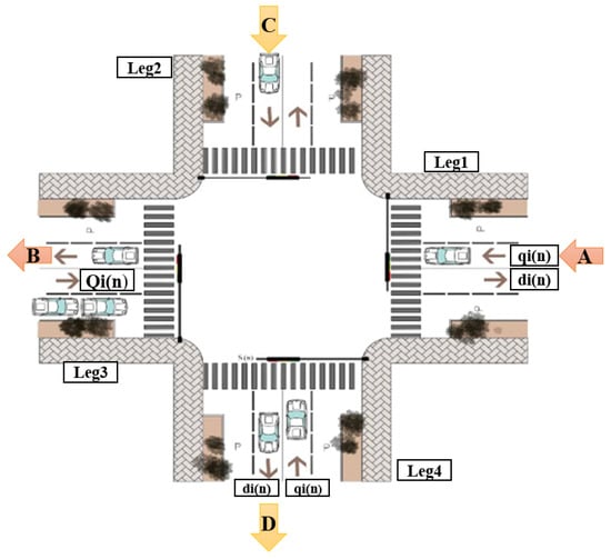
Figure 1. A two-phase signal at an intersection.

In Equation (1), $i=1,2,3,\dots ,n$ represents the legs at an intersection with four legs. The first is leg 1, the second is leg 2, the third is leg 3, and the fourth is leg 4. At this intersection, cars are the input and output. The greater the number of entrances and exits from one leg to another, the more traffic increases. According to Figure 1, the vehicles enter from A, from the leg in that direction, and exit from B, thus entering the third leg. In leg 2, the cars enter from C and exit from D, entering leg 4. At this intersection, the issue of queue length is an important parameter in traffic flow. Vehicles are inputs to a leg and outputs from another leg and increase the length of the vehicles’ queue. As mentioned in this case, the length of the queue is one of the important parameters of the traffic flow, which indicates the state and traffic situation at an intersection and is represented as follows.

$$Q_i(n+1)=Q_i\left(n\right)+q_i\left(n\right)-d_i\left(n\right)s_i\left(n\right)$$

(1)

where $i=1,2,3,\dots ,n$ is the index of legs at the intersection; $n=0,1,2,\dots ,N-1$ is the index of discrete time intervals; N is the horizon of the simulation; $Q_i\left(n\right)$ is the length of the queue consisting of the number of vehicles; $q_i\left(n\right)$ is the number of vehicles entering the queue as inputs; and $d_i\left(n\right)$ is the number of vehicles leaving the queue as outputs. Each intersection has a traffic light that indicates the status of the control signal at the intersection. Legs 1 and 3 have a connected traffic light, and legs 2 and 4 have a connected traffic light. $s_i\in [0,1]$ indicates the status of the signal at an intersection. When $s=1$, the traffic light is green and vehicles move; when $s=0$, the light is red and vehicles are stopped. According to Figure 1, at the intersection, a signal status of $s1,s2,s3,s4=(0,1,0,1)$ means that the traffic light is green in lanes 1 and 3 and red in lanes 2 and 4 and, as a result, vehicles can move in lanes 1 and 3 but are stopped in lanes 2 and 4. If T is considered the discretized time interval and is short enough, then the vehicle’s arrival can be assumed uniform at every time interval, and as a result, the overall wait time of vehicles is calculated using Equation (2):

$$W_i(n+1)=W_i+TQi\left(n\right)+q_i\left(n\right)-d_i\left(n\right)s_i\left(n\right)1/2q_i\left(n\right)$$

(2)

where $W_i\left(n\right)$ is the average vehicle wait time of i queue from the beginning of the average period to the onset of n time interval. The wait time and the number of vehicles are popular performance indices for the signal controls defined in Equation (2). To facilitate its formulation, the state-space equations and the optimization objective can be rewritten in the matrix form as follows:

$$\left\{\begin{array}{c}X(n+1)=AX\left(n\right)+B\left(n\right)S+C\left(n\right)\\ Y\left(n\right)=CX\left(n\right)\end{array}\right.$$

(3)

where

$$W_i(n+1)=W_i+TQi\left(n\right)+q_i\left(n\right)-d_i\left(n\right)s_i\left(n\right)1/2T{q}_i\left(n\right)$$

(4)

$$X\left(n\right)={[Q_1\left(n\right)Q_2\left(n\right)\dots Q_M\left(n\right)W_1\left(n\right)W_2\left(n\right)\dots W_M\left(n\right)]}^T$$

(5)

are the vectors of state variables and

$$S\left(n\right)={[S_1\left(n\right)S_2\left(n\right)\dots S_M\left(n\right)]}^T.$$

(6)

Various coefficient matrices and vectors were considered, which are as follows:

$$C=\left[\begin{array}{cc}{I}_M& 0\\ 0& I_M\end{array}\right]$$

(7)

$$A=\left[\begin{array}{cc}{I}_M& 0\\ T{I}_M& I_M\end{array}\right]$$

(8)

$$B\left(n\right)=-\left[\begin{array}{cccccc}{d}_1\left(n\right)& 0& .& .& .& 0\\ 0& d_2\left(n\right)& .& .& .& 0\\ .& .& .& .& .& .\\ .& .& .& .& .& .\\ .& .& .& .& .& .\\ 0& .& .& .& .& d_M\left(n\right)\\ 1/2T{d}_1\left(n\right)& 0& .& .& .& 0\\ 0& 1/2T{d}_2\left(n\right)& 0& 0& 0& 0\\ .& .& .& .& .& .\\ .& .& .& .& .& .\\ .& .& .& .& .& .\\ 0& 0& .& .& .& 1/2T{d}_M\left(n\right)\end{array}\right]$$

(9)

$$C_n={[q_1\left(n\right)q_2\left(n\right)\dots q_M\left(n\right)1/2T{q}_1\left(n\right)1/2T{q}_2\left(n\right)\dots 1/2T{q}_M\left(n\right)]}^T$$

(10)

where

$$X\left(n\right)={[Q_1\left(n\right)Q_2\left(n\right)\dots Q_M\left(n\right)W_1\left(n\right)W_2\left(n\right)\dots 1/2T{q}_M\left(n\right)]}^T.$$

(11)

are state variables and $Q_i\left(n\right)$ denotes the queue length and delays in vehicles.

4. Data

According to the Table 2, the data were divided into two main parts: components and the number of components. The data are described in summary below:

Table 2. Data.

Components	Total Number
Number of data	1000
Total length	4
Signal traffic	0 and 1

• The data contain the queue length and traffic signal.
• The data consist of four main parts in a signal intersection. In a simulation of the proposed model, each traffic light cycle’s sampling time was $0.1$ s.
• The simulation was executed in under 100 s. This shows that the queue length was reduced by a fixed amount of time using controller design data.
• This process was considered randomly at one of the intersections in Tehran, Iran.

5. Controller Design

Predictive control is a model-based controller affecting model accuracy significantly. It can apply constraints on both input and output signals and can control signal generation. It can also be easily used in multivariate systems. The general diagram of the predictive control is shown in Figure 2.

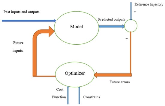
Figure 2. General diagram of model predictive control.

The predictive control structure has a process model, cost function, and control law. The predictive control was derived from a set of control rules such as predicting the future output of a system over a specified period using the initial process model of computed control signals in the forecast horizon by minimizing a cost function and by applying the first control signal, then calculating it within the system, and repeating the whole process in the next steps. The main purpose is to predict the queue length decrease concerning future system inputs at each sampling time, optimizing the system’s future behavior. In this controller, the inputs include the length of the queue of vehicles and the number of inbound and outbound vehicles per leg. The state-space equation is defined in Equation (3). T indicates an optional sampling time. Assume that the sampling time is sufficiently uniform when the vehicle arrives at any time interval and that the intersection has four legs. Each leg has three lines, the vehicles are independent in each line, and a normal distribution is used for generating inputs. The cost function is defined as follows:

$$J=X^T(n+1)QX(n+1)\mathsf{\Delta }{S}^T\left(n\right)W\mathsf{\Delta }S\left(n\right)$$

(12)

and we suggest:

$$\mathsf{\Delta }S={(-2(\mathsf{\Delta }{X}^T{A}^T{\xi }^{T}B+C^T{\xi }^T\xi B){(B^T{\xi }^T\xi B+R^T)}^{-1})}^T$$

(13)

Theorem 1.

Consider the dynamic equation in Equation (3), which satisfies the above assumptions. The control input in Equation (13) that minimizes the cost function in Equation (12) causes the vehicles in the queue of each leg to be constrained in all four directions.

Proof. 

Sustainability of this model is proven as follows:

$$\left(\begin{array}{c}\mathsf{\Delta }(n+1)\\ Y\left(n\right)\end{array}\right)=\left(\begin{array}{cc}A& 0\\ C& I\end{array}\right)\left(\begin{array}{c}\mathsf{\Delta }(n+1)\\ Y\left(n\right)\end{array}\right)+\left(\begin{array}{c}B\\ 0\end{array}\right)+\left(\begin{array}{c}I\\ 0\end{array}\right)\mathsf{\Delta }C\left(n\right)$$

(14)

$$y^{\prime }\left(n\right)=\left[\begin{array}{ccc}[cI& 0]& 0\end{array}\right]\left(\begin{array}{c}\mathsf{\Delta }X\left(n\right)\\ y\left(n\right)\end{array}\right)$$

(15)

Equations (14) and (15) show the output-based prediction in a previous sample, according to which the forward state vectors of the future state are defined as follows:

$$\begin{array}{cc}\hfill x(n_i+1|n_i)=Ax\left(n_i\right)+B\mathsf{\Delta }S\left(n_i\right)+\mathsf{\Delta }C\left(n_i\right)& \hfill =\\ \hfill Ax(n_i+1|n_i)+B\mathsf{\Delta }S(n_i+1|n_i)+C(n_i+1|n_i)& \hfill =\\ \hfill A^{2}x\left(n_i\right)+AB\mathsf{\Delta }S\left(n_i\right)+B\mathsf{\Delta }S(n_i+1)+AC\left(n_i\right)+C(n_i+1)\end{array}$$

(16)

Continue the equation to $N_P$:

$$\begin{array}{cc}\hfill x(n_i+N_p|n_i)=A^{N_p}x\left(n_i\right)+A^{N_p-1}B\mathsf{\Delta }S\left(n_i\right)& +\hfill \\ \hfill A^{N_p-2}B\mathsf{\Delta }S(n_i+1)+A^{N_p-N_c}B\mathsf{\Delta }S(n_i+N_c-1)& +\hfill \\ \hfill A^{N_p}C\left(n_i\right)+A^{N_p}C(n_i+1|n_i)+\dots +C(n_i+N_P-1|n_i)\end{array}$$

Considering the predicted state vectors, the predicted output is expressed as follows:

$$\begin{array}{c}\hfill y(n_i+1|n_i)=CAx\left(n_i\right)+CB\mathsf{\Delta }S\left(n_i\right)+C\mathsf{\Delta }n\left(n_i\right)y(n_i+2|n_i)=\\ \hfill C{A}^{2}x\left(n_i\right)+CAB\mathsf{\Delta }S\left(n_i\right)\&+CB\mathsf{\Delta }S(n_i+1)+C\mathsf{\Delta }C(n_i+1)\end{array}$$

(17)

Continue the equation to $N_P$:

$$\begin{array}{c}\hfill y(n_i+N_p|n_i)=C{A}^{N_p}x\left(n_i\right)+C{A}^{N_p-1}B\mathsf{\Delta }S\left(n_i\right)+C{A}^{N_p-2}B\mathsf{\Delta }S(n_i+1)+\\ \hfill \dots +C{A}^{N_p-N_c}B\mathsf{\Delta }S(n_i+N_c-1)+C{A}^{N_p-1}\mathsf{\Delta }C\left(n_i\right)+C\mathsf{\Delta }C(n_i+1)\end{array}$$

By combining Equations (14)–(17), we can show the output prediction vector as follows:

$$Y=Fx\left(n_i\right)+\varphi \mathsf{\Delta }S$$

(18)

$$Y=\left[\begin{array}{c}CA\\ C{A}^2\\ .\\ .\\ .\\ C{A}^{N_p}\end{array}\right]$$

(19)

$$\varphi =\left[\begin{array}{cccccc}CB& 0& .& .& .& 0\\ CAB& CB& .& .& .& 0\\ C{A}^{2}B& CAB& .& .& .& .\\ .& .& .& .& .& .\\ .& .& .& .& .& .\\ .& .& .& .& .& .\\ C{A}^{N_p-1}B& C{A}^{N_p-2}B& .& .& .& C{A}^{N_p-N_c}B\end{array}\right]$$

(20)

$$C=\left[\begin{array}{cccccc}C& 0& .& .& .& 0\\ CA& C& .& .& .& 0\\ C{A}^2& CA& .& .& .& .\\ .& .& .& .& .& .\\ .& .& .& .& .& .\\ .& .& .& .& .& .\\ C{A}^{N_p-1}& C{A}^{N_p-2}& .& .& .& C{A}^{N_p-N_c}\end{array}\right]$$

(21)

The optimization based on Equation (15) is given by considering a four-way path:

$$\mathsf{\Delta }{x}_m\left(n\right)=\left[\begin{array}{c}{Q}_1\\ .\\ .\\ .\\ Q_M\\ W_1\\ .\\ .\\ .\\ W_M\end{array}\right]$$

(22)

$$y^{\prime }=\left[\begin{array}{cccccccc}1& 1& 1& 1& 0& 0& 0& 0\end{array}\right]\left[\begin{array}{c}\mathsf{\Delta }{x}_1\left(n\right)\\ .\\ .\\ .\\ \mathsf{\Delta }{x}_8\left(n\right)\end{array}\right]=1\left(\mathsf{\Delta }{x}_1\left(n\right)\right)+\dots +\mathsf{\Delta }{x}_4\left(n\right))+0$$

(23)

$$H={y\prime }^{T}y+\mathsf{\Delta }{S}^{T}R\mathsf{\Delta }S$$

(24)

Additionally, by putting Equations (22) and (23) into Equation (24), we obtain the following:

$$H={\left(\xi \mathsf{\Delta }X(n+1)\right)}^T\left(\xi \mathsf{\Delta }X(n+1)\right)+\mathsf{\Delta }{S}^{T}R\mathsf{\Delta }S$$

(25)

In Equation (24), $\xi$= [1 1 1 1 0 0 0 0] is considered and results in the following:

$$\mathsf{\Delta }X(n+1)=A\mathsf{\Delta }X+B\mathsf{\Delta }S+C$$

(26)

In Equation (14), we obtain the following:

$$H={(A\mathsf{\Delta }X+B\mathsf{\Delta }S+C)}^T{\xi }^T\xi (A\mathsf{\Delta }X+\mathsf{\Delta }S+C)+\mathsf{\Delta }{S}^{T}R\mathsf{\Delta }S$$

(27)

Finally, by deriving the cost function of the control effort and by equalizing Equation (28), we have the following:

$$\frac{\partial H}{\partial \mathsf{\Delta }S}=0$$

(28)

The result is shown as follows in Equations (28) and (29).

$$\begin{array}{cc}\hfill \partial H/\partial \mathsf{\Delta }S=\mathsf{\Delta }{X}^T{A}^T{\xi }^T\xi B+\mathsf{\Delta }{X}^T{A}^T{\xi }^T\xi B& +\hfill \\ \hfill \mathsf{\Delta }{S}^T{B}^T{\xi }^T\xi B+C^T{\xi }^T\xi B+\mathsf{\Delta }{S}^T(R+R^T)=0\end{array}$$

(29)

From Equation (28), the optimal solution is obtained to compute the control effort. □

6. Simulation Results

The simulation aims to reduce the queue length of vehicles at an intersection with two constant-time modes using a predictive model based on a steady-state intelligent controller and sampling time $T=0.1$s. Table 3 shows the different traffic positions with specified values of $\beta$.

Table 3. Values at different traffic positions $\beta$.

Traffic Status	$\mathit{\beta }$
No Saturation	$\beta$ >= 0.7
Saturation	0.4 <=$\beta$ <= 0.6
Over-Saturated	0.1 <=$\beta$ <= 0.3
Unstable	0 = $\beta$

The following equation gives the number of vehicles departing from the line to the interval:

$$d_i\left(n\right)=min(Q_i\left(n\right)+q_i\left(n\right),d_{si}\left(n\right))$$

(30)

Additionally, the saturation flow rate over time interval T is as follows:

$$d_{si}\left(n\right)=d_{cons}\left(n\right)+\beta q_i\left(n\right),i=0,1,2,3,4$$

(31)

The parameters $d_{cons}$ >= 50 and 0 <= $\beta$ <= 1 can be randomly defined as $q_i$, $d_i$ in Equation (26). The simulation results are compared to constant time control using the designed control.

6.1. Constant Time Control

In constant time control, the simulation results for the number of vehicles in the line without the use of the controller are such that the control variables represent the green and red timing of the traffic light in a four-way direction. In this case, red represents the traffic light at the first and third legs in Figure 3 while green represents the traffic light at the second and fourth legs in Figure 4.

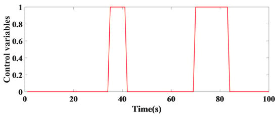
Figure 3. The traffic light is red at the first and third legs of a single intersection.

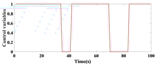
Figure 4. The traffic light is green at the second and fourth legs of a single intersection.

The lengths of the vehicle queue at the first leg in Figure 5 and at the second leg in an intersection in Figure 6 are presented, indicating constant time control and improving the predictive controller.

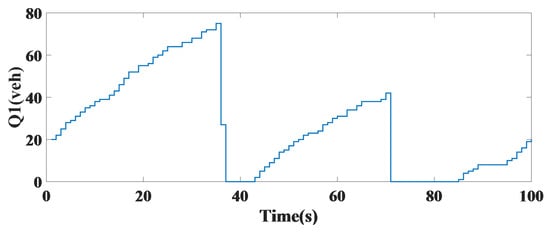
Figure 5. The length of the vehicle queue at the first leg of a single intersection.

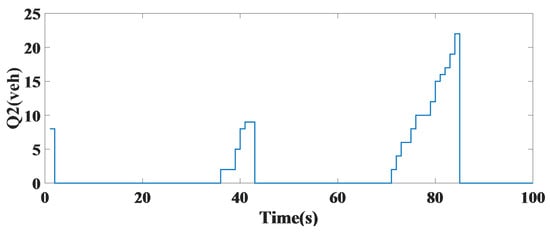
Figure 6. The length of the vehicle queue at the second leg of a single intersection.

Figure 7 shows the number of vehicles in the third leg at a single intersection with constant time control, initially increasing and then decreasing in length over time.

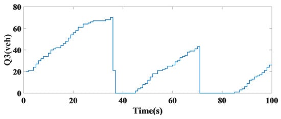
Figure 7. The length of the queue of vehicles in the third leg of a single intersection.

In Figure 8, the volume of traffic generated in the fourth leg also increased over time.

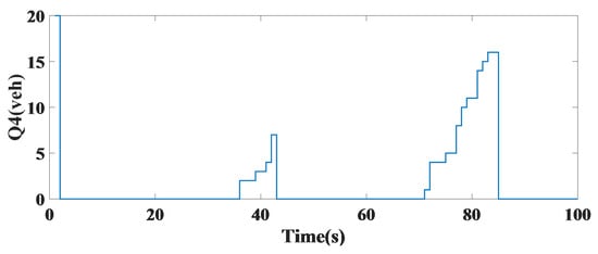
Figure 8. Vehicle queue length at the fourth leg of a single intersection.

6.2. Model-Based Predictive Smart Controller

In this section, the controller designed in Equation (10) was implemented in an intersection’s dynamic system. As shown in Figure 9 and Figure 10, the control variables represent when the traffic light is green or red by applying a model-based predictor controller at an intersection.

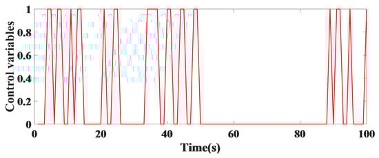
Figure 9. Traffic light being green or red for the first and third legs of a single intersection.

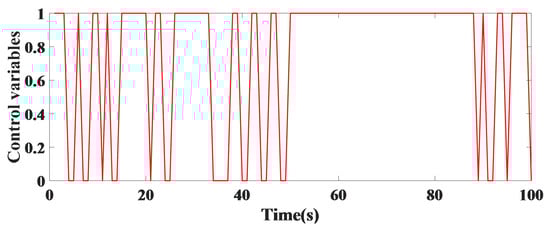
Figure 10. Traffic light being green or red for the second and fourth legs of a single intersection.

The length of the vehicle queue within the first stretch of an intersection is reduced when the controller is implemented compared to that for the case without the controller, as shown in Figure 10. The vehicle queue length at the second leg of the intersection in the case using the controller decreased significantly without considering constant time, as shown in Figure 11.

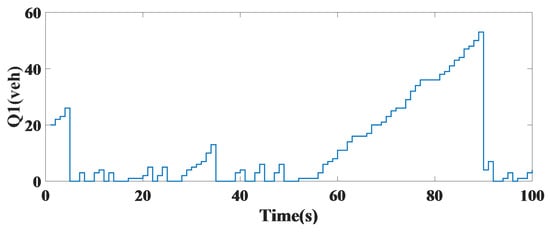
Figure 11. The length of the vehicle queue for the first leg of a single intersection.

The length of the vehicle queue at the third leg of the crossing shown in Figure 12 where the controller was applied was minimized and somewhat improved.

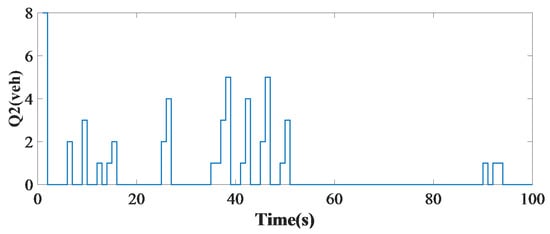
Figure 12. The length of the vehicle queue at the second leg of a single intersection.

Figure 13 shows the length of the vehicle queue at the fourth leg of an intersection. The number of vehicles in the traffic queue is reduced to a minimum using the predictive controller; it decreased significantly compared to the non-controller mode.

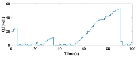
Figure 13. The length of the vehicle queue at the third leg of a single intersection.

The length of the car queue at each leg was compared with the fixed-time control method at each of the four legs using the predictive controller and the number of vehicles in terms of sampling time per $0.1$ s. In the first leg, the number of vehicles stationary in the four-way intersection was reduced to 3 using the controller. In the second leg, the number of vehicles was reduced from 21 to 1. Additionally, in the third leg, the number of vehicles using a steady-state model decreased from 70 to 7 using the predictive controller to improve the queue. The fourth leg of the intersection minimized the number of vehicles optimally, as seen in Figure 14. In Table 4, the results are shown with constant time control and the predictive controller.

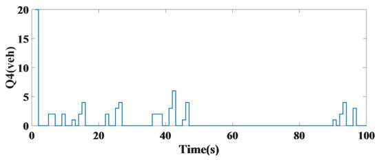
Figure 14. The length of the vehicle queue in the fourth leg of a single intersection.

Table 4. A comparison of the results for the length of the vehicle queue using model predictive control at an intersection.

Queue Length Vehicles	Q1	Q2	Q3	Q4	Total
Control fixed time	62	21	70	16	169
Model predictive control	3	1	7	4	15
Improvement percentage	95.23	95.23	94.78	75	91.12

7. Conclusions

In this paper, a model predictive controller was designed to generate and tune traffic light signals at an intersection and their stability was investigated. Among the advantages of the model proposed, model predictive control has the ability to compensate for low-traffic times and it identifies reference paths for use in the future. The proposed model predictive controller was designed for an intersection based on two basic parameters that determine the length of a queue, and vehicle latency was considered. We studied the stability of the intersection using model predictive control, and the Hamiltonian equation was used to prove this stability. By applying a controller based on discrete-time state-space equations, the length of the vehicle queue was minimized compared to the fixed-time mode, and the volume created in each leg also obtained similar results. The proposed method had a better performance compared to the fixed-time controller in all lanes of the intersection. Moreover, the effectiveness of the proposed controller was proven via simulation results.

References

- Ye, B.L.; Wu, W.; Ruan, K.; Li, L.; Chen, T.; Gao, H.; Chen, Y. A survey of model predictive control methods for traffic signal control. IEEE/CAA J. Autom. Sin. 2019, 6, 623–640. [Google Scholar] [CrossRef]
- Sumi, L.; Ranga, V. Intelligent traffic management system for prioritizing emergency vehicles in a smart city. Int. J. Eng. 2018, 31, 278–283. [Google Scholar]
- Li, D.; Deng, L.; Cai, Z.; Franks, B.; Yao, X. Intelligent transportation system in Macao based on deep self-coding learning. IEEE Trans. Ind. Inform. 2018, 14, 3253–3260. [Google Scholar] [CrossRef]
- Khan, P.W.; Byun, Y.C.; Park, N. A data verification system for CCTV surveillance cameras using blockchain technology in smart cities. Electronics 2020, 9, 484. [Google Scholar] [CrossRef]
- Khan, P.W.; Byun, Y.C. Smart contract centric inference engine for intelligent electric vehicle transportation system. Sensors 2020, 20, 4252. [Google Scholar] [CrossRef] [PubMed]
- Chedjou, J.C.; Kyamakya, K. A review of traffic light control systems and introduction of a control concept based on coupled nonlinear oscillators. Recent Adv. Nonlinear Dyn. Synchronization 2018, 109, 113–149. [Google Scholar]
- Papageorgiou, M.; Diakaki, C.; Dinopoulou, V.; Kotsialos, A.; Wang, Y. Review of road traffic control strategies. Proc. IEEE 2003, 91, 2043–2067. [Google Scholar] [CrossRef]
- Araghi, S.; Khosravi, A.; Creighton, D. A review on computational intelligence methods for controlling traffic signal timing. Expert Syst. Appl. 2015, 42, 1538–1550. [Google Scholar] [CrossRef]
- Zhao, D.; Dai, Y.; Zhang, Z. Computational intelligence in urban traffic signal control: A survey. IEEE Trans. Syst. Man Cybern. Part C (Appl. Rev.) 2011, 42, 485–494. [Google Scholar] [CrossRef]
- Zhao, H.; Han, G.; Niu, X. The signal control optimization of road intersections with slow traffic based on improved PSO. Mob. Netw. Appl. 2019, 1–9. [Google Scholar] [CrossRef]
- Silva, C.M.; Aquino, A.L.; Meira, W. Smart traffic light for low traffic conditions. Mob. Netw. Appl. 2015, 20, 285–293. [Google Scholar] [CrossRef]
- Ye, B.L.; Wu, W.; Gao, H.; Lu, Y.; Cao, Q.; Zhu, L. Stochastic model predictive control for urban traffic networks. Appl. Sci. 2017, 7, 588. [Google Scholar] [CrossRef]
- Dongling, X.; Jianan, F.; Shihuang, S. A fuzzy controller of traffic systems and its neural network implementation. Inf. Control 1992, 2. Available online: https://en.cnki.com.cn/Article_en/CJFDTotal-XXYK199202001.htm (accessed on 10 February 2021).
- “Brian” Park, B.; Messer, C.J.; Urbanik, T., II. Enhanced genetic algorithm for signal-timing optimization of oversaturated intersections. Transp. Res. Rec. 2000, 1727, 32–41. [Google Scholar] [CrossRef]
- Fiore, M. Mobility models in inter-vehicle communications literature. Politec. Torino 2006, 147. Available online: http://citeseerx.ist.psu.edu/viewdoc/download?doi=10.1.1.103.4702&rep=rep1&type=pdf (accessed on 17 May 2021).
- Lin, S.; De Schutter, B.; Xi, Y.; Hellendoorn, H. Fast model predictive control for urban road networks via MILP. IEEE Trans. Intell. Transp. Syst. 2011, 12, 846–856. [Google Scholar] [CrossRef]
- Li, X.; Sun, J.Q. Multi-objective optimal predictive control of signals in urban traffic network. J. Intell. Transp. Syst. 2019, 23, 370–388. [Google Scholar] [CrossRef]
- Zhou, X.; Ye, B.L.; Lu, Y.; Xiong, R. A novel MPC with chance constraints for signal splits control in urban traffic network. IFAC Proc. Vol. 2014, 47, 11311–11317. [Google Scholar] [CrossRef]
- de Souza, F.A.; Camponogara, E.; Kraus, W.; Peccin, V.B. Distributed MPC for urban traffic networks: A simulation-based performance analysis. Optim. Control. Appl. Methods 2015, 36, 353–368. [Google Scholar] [CrossRef]
- Jiang, T.; Wang, Z.; Chen, F. Urban Traffic Signals Timing at Four-Phase Signalized Intersection Based on Optimized Two-Stage Fuzzy Control Scheme. Math. Probl. Eng. 2021, 2021. [Google Scholar] [CrossRef]
- Li, L.; Okoth, V.; Jabari, S.E. Backpressure control with estimated queue lengths for urban network traffic. IET Intell. Transp. Syst. 2021, 15, 320–330. [Google Scholar] [CrossRef]
- Radivojević, M.; Tanasković, M.; Stević, Z. The adaptive algorithm of a four way intersection regulated by traffic lights with four phases within a cycle. Expert Syst. Appl. 2021, 166, 114073. [Google Scholar] [CrossRef]
- Dai, Z.; Song, H.; Liang, H.; Wu, F.; Wang, X.; Jia, J.; Fang, Y. Traffic parameter estimation and control system based on machine vision. J. Ambient. Intell. Humaniz. Comput. 2020, 1–13. [Google Scholar] [CrossRef]
- Jin, J.; Ma, X. Hierarchical multi-agent control of traffic lights based on collective learning. Eng. Appl. Artif. Intell. 2018, 68, 236–248. [Google Scholar] [CrossRef]
- Rastgoftar, H.; Jeannin, J.B. A Physics-Based Finite-State Abstraction for Traffic Congestion Control. arXiv 2021, arXiv:2101.07865. [Google Scholar]
- Wu, N.; Li, D.; Xi, Y.; de Schutter, B. Distributed event-triggered model predictive control for urban traffic lights. IEEE Trans. Intell. Transp. Syst. 2020. [Google Scholar] [CrossRef]
- Zuo, Z.; Yang, X.; Li, Z.; Wang, Y.; Han, Q.; Wang, L.; Luo, X. MPC-based Cooperative Control Strategy of Path Planning and Trajectory Tracking for Intelligent Vehicles. IEEE Trans. Intell. Veh. 2020. [Google Scholar] [CrossRef]
- van de Weg, G.S.; Keyvan-Ekbatani, M.; Hegyi, A.; Hoogendoorn, S.P. Linear MPC-Based Urban Traffic Control Using the Link Transmission Model. IEEE Trans. Intell. Transp. Syst. 2019, 21, 4133–4148. [Google Scholar] [CrossRef]
- Lu, K.; Du, P.; Cao, J.; Zou, Q.; He, T.; Huang, W. A novel traffic signal split approach based on explicit model predictive control. Math. Comput. Simul. 2019, 155, 105–114. [Google Scholar] [CrossRef]
- Wang, Q.; Abbas, M. Optimal urban traffic model predictive control for nema standards. Transp. Res. Rec. 2019, 2673, 413–424. [Google Scholar] [CrossRef]
- Yao, N.; Zhang, F. Contention-resolving model predictive control for an intelligent intersection traffic model. Discret. Event Dyn. Syst. 2021, 1–31. [Google Scholar] [CrossRef]
- HomChaudhuri, B.; Vahidi, A.; Pisu, P. Fast model predictive control-based fuel efficient control strategy for a group of connected vehicles in urban road conditions. IEEE Trans. Control. Syst. Technol. 2016, 25, 760–767. [Google Scholar] [CrossRef]
- Wu, C.Y.; Hu, M.B.; Jiang, R.; Hao, Q.Y. Effects of road network structure on the performance of urban traffic systems. Phys. A Stat. Mech. Its Appl. 2021, 563, 125361. [Google Scholar] [CrossRef]
- El Hatri, C.; Boumhidi, J. Fuzzy deep learning based urban traffic incident detection. Cogn. Syst. Res. 2018, 50, 206–213. [Google Scholar] [CrossRef]
- Li, C.; Xu, P. Application on traffic flow prediction of machine learning in intelligent transportation. Neural Comput. Appl. 2021, 33, 613–624. [Google Scholar] [CrossRef]
- Qiao, F.; Liu, T.; Sun, H.; Guo, L.; Chen, Y. Modelling and simulation of urban traffic systems: Present and future. Int. J. Cybern. Cyber-Phys. Syst. 2021, 1, 1–32. [Google Scholar] [CrossRef]
- Shahbazi, Z.; Byun, Y.C. A Procedure for Tracing Supply Chains for Perishable Food Based on Blockchain, Machine Learning and Fuzzy Logic. Electronics 2021, 10, 41. [Google Scholar] [CrossRef]
- Shahbazi, Z.; Byun, Y.C. Improving Transactional Data System Based on an Edge Computing–Blockchain–Machine Learning Integrated Framework. Processes 2021, 9, 92. [Google Scholar] [CrossRef]
- Zhou, C.; Mo, H.; Chen, X.; Wen, H. Fuzzy Control Under Time-Varying Universe and Phase Optimization in Traffic Lights (ICSSE 2020). Int. J. Fuzzy Syst. 2021, 1–12. [Google Scholar] [CrossRef]
- Shahbazi, Z.; Byun, Y.C. Smart Manufacturing Real-Time Analysis Based on Blockchain and Machine Learning Approaches. Appl. Sci. 2021, 11, 3535. [Google Scholar] [CrossRef]
- Xu, M.; Chai, J.; Yan, Y.; Qu, X. Multi-Agent Fuzzy-Based Transit Signal Priority Control for Traffic Network Considering Conflicting Priority Requests. IEEE Trans. Intell. Transp. Syst. 2021. [Google Scholar] [CrossRef]
- Xu, M.; An, K.; Vu, L.H.; Ye, Z.; Feng, J.; Chen, E. Optimizing multi-agent based urban traffic signal control system. J. Intell. Transp. Syst. 2019, 23, 357–369. [Google Scholar] [CrossRef]
- Shahbazi, Z.; Byun, Y.C. Integration of Blockchain, IoT and Machine Learning for Multistage Quality Control and Enhancing Security in Smart Manufacturing. Sensors 2021, 21, 1467. [Google Scholar] [CrossRef] [PubMed]
- Azimirad, E.; Pariz, N.; Sistani, M.B.N. A novel fuzzy model and control of single intersection at urban traffic network. IEEE Syst. J. 2010, 4, 107–111. [Google Scholar] [CrossRef]
- Arehpanahi, M.; Fazli, M. Position control improvement of permanent magnet motor using model predictive control. Int. J. Eng. 2018, 31, 1044–1049. [Google Scholar]
- Akbar Ghafouri Rokn Abadi, A. Constrained model predictive control of low-power industrial gas turbine. Int. J. Eng. 2017, 30, 207–214. [Google Scholar]
- Shahbazi, Z.; Byun, Y.C. Topic prediction and knowledge discovery based on integrated topic modeling and deep neural networks approaches. J. Intell. Fuzzy Syst. 2021, 1–17. [Google Scholar] [CrossRef]
Publisher’s Note: MDPI stays neutral with regard to jurisdictional claims in published maps and institutional affiliations. |
© 2021 by the authors. Licensee MDPI, Basel, Switzerland. This article is an open access article distributed under the terms and conditions of the Creative Commons Attribution (CC BY) license (https://creativecommons.org/licenses/by/4.0/).