A Pro-Environmental Method of Sample Size Determination to Predict the Quality Level of Products Considering Current Customers’ Expectations

Abstract

The main factor that conditions the success of organizations is the development of products oriented toward customer satisfaction. An additional attribute of organizations is the use of sustainable development rules. The use of these rules and the simultaneous desire to create high-quality products encourage organizations to apply different methods to, for example, eliminate waste. This study aimed to develop a method to determine the research sample size required to predict a product’s quality level, taking into account current customers’ expectations. This method was developed by modifying a procedure to determine the research sample size as part of the calculated estimator of the mean value in the general population. Based on the concept of product sustainability development, the goal of the developed method was to determine the number of potential customers (respondents) needed to provide product requirements, which were then processed and used to predict the quality level of the product. This method was applied to simultaneously test a number of hypotheses, determine the test power, and detect statistically significant differences for several relationships of the sample sizes and the test power. This was achieved using universal hypotheses and the popular alternative-punctual (MAP) method. Testing of the proposed method showed that it was able to predict the quality level of products based on current expectations of customers.

1. Introduction

Due to dynamic technological changes and a competitive environment, the development of products oriented toward customers is a growing trend in the production field [1,2,3,4]. This orientation includes customer expectations to ensure a satisfactory level of product quality. Mentioned product quality level is referred to the compatibility of product with customers’ requirements and it concerns only concrete intended use of the product. The quality of product is determined, e.g., with including customers’ satisfaction, that is, customers’ contentment from what received (current product) and what expected (future product). In turn, the aforementioned customer expectations concern what the customers want, believes, and expects in the context of the future. Simultaneously, pro-environmental changes are taking place at the society level, which are mainly manifested by the use of sustainability rules. This coexistence of aspirations to achieve high quality and sustainable development appears to be a natural competitive action of any well-managed organization [4,5,6], which concerns the sustainable design of new products and improvement of the quality level of existing products [7,8,9,10,11]. This process not only results in higher satisfaction of customers and good economic results, but also, and most importantly, the effective implementation of sustainable development [12,13,14,15,16]. In this context, there appears to be a lack of a single, consistent method that allows the determination of the number of customers from whom expectations should be obtained to predict a product’s quality level.

A literature review of this subject indicates that methods to determine the research sample size were used to test preconceived hypotheses [17,18,19,20,21,22,23]. In addition, customer requirements have been obtained using, for example, traditional methods, such as interviews or survey research [24,25]. Other tools have also been used; for example, the ladder technique to trigger customer requirements using the so-called customer attribute hierarchy (CAH) [26,27]. The Delphi method has been used [28] to select the most important product features according to the customer. In previous research [29], the DBC method has been used, which allows for customers to participate in the process of product design, resulting in modification and adjustment of the product to the customers’ requirements. Therefore, in the context of processing and determination of products’ quality level, the main methods used have been Kansei (KE) [24,30,31,32], Quality Function Deployment (QFD) [33,34,35,36], Kano [16,34,37,38], and the Bayesian Network (Naive Bayesian Classifier) [39,40,41,42,43]. These methods were also integrated [31,32,34,38,44]. The use of the Kansei method (KE) [24,30,31,32] included determination of the psychology of customers, and then matching customers to Kansei words. This method was integrated with the QFD method to precisely determine both quantitative (technical) and qualitative (emotional) requirements [31,44]. In addition, the Kansei method was integrated with the Kano model [32] to organize product features into categories in accordance with customer requirements. The mentioned QFD method (Quality Function Deployment or Product Planning House of Quality (PPHOQ)) [38] has been widely used to translate customer requirements onto the technical attributes of a product [33,34,35,36]. For example, the authors of article [35] presented the QFD method for ordering the importance of customer requirements, taking into account information about the competition. Another example is article [34], in which authors integrated the QFD method with the Kano model to quantitatively and qualitatively analyze the relationship between the requirements and satisfaction of the customer. In turn, the mentioned Kano model [16,34,37,38] has been applied to the qualitative analysis of customer requirements [45] and the improvement of products [46]. This approach allows identification of attractive or mandatory requirements in accordance with customers’ needs; however, it is not possible to identify a degree of satisfaction or dissatisfaction with the features of a product [37]. In article [38], the authors combined the Kano model with other techniques, i.e., rough set theory, the analytical hierarchy process (AHP) [47], and the scale method [38], to precisely define the requirements of customers as part of the House of Quality (QFD). In turn, the above-mentioned Bayesian network (i.e., the so-called Naive Bayesian Classifier), is a probabilistic classifier based on independent, conditional assumptions. Examples in the literature, e.g., [39,40,41,42,43], apply the Bayesian network to adjust the level of product quality to meet customers’ requirements. Forecasting or prediction of products’ quality level has been analyzed in which authors applied a hidden Markov chain model [16,33,36]. The aim was to analyze the past and present customer requirements from a set of probabilities to predict the requirements of customers. Additionally, with the same aim, the Markov chain model was integrated with the Kano model and grey theory [16].

Following this literature review, it was concluded that previous research has determined the required number of customers [17,18,19,20,21,22,23]; furthermore, customers’ expectations have been obtained and processed to determine the quality level of products (for example: [24,25,30,34,35,38]). Methods to forecast or predict the quality level of products have also been implemented [27,33,36]. However, these studies did not use a single, consistent method that would allow the determination of the number of customers from whom expectations should be obtained, so that a product’s quality level can be predicted. This indicates the lack of a consistent method to determine the sample size for prediction of a product’s quality level, taking into account customers’ expectations. Therefore, the aim of this article is to propose a method to determine the research sample size to predict a product’s quality level, taking into account current customer expectations. This approach results from modification of a method used to determine the size of the research sample, thus helping to fulfil the rules of sustainable development and meet the aim of organizations to maximize quality. Therefore, two theses were adopted:

Thesis 1.

It is possible to determine the number of customers from whom expectations should be obtained and processed to predict a product’s quality level, taking into account customers’ expectations. This prediction encompasses both actual and modified product quality levels.

Thesis 2.

It is possible to determine the sample size required to predict the product quality level taking into account customers’ expectations, in addition to determining the sample size to test a number of hypotheses, providing a test power for this sample size, and detecting the statistically significant differences for several relationships between this sample size and the test power.

To verify these theses, a test was undertaken of the proposed method for predicting a product’s quality product level taking into account current customers’ expectations.

This method is ideal for the topic under investigation, because is a single method that allows to addiction the sample size into the modification of product attributes, and customers’ satisfaction from quality product level for these modifications in the context of predicting future design product changes.

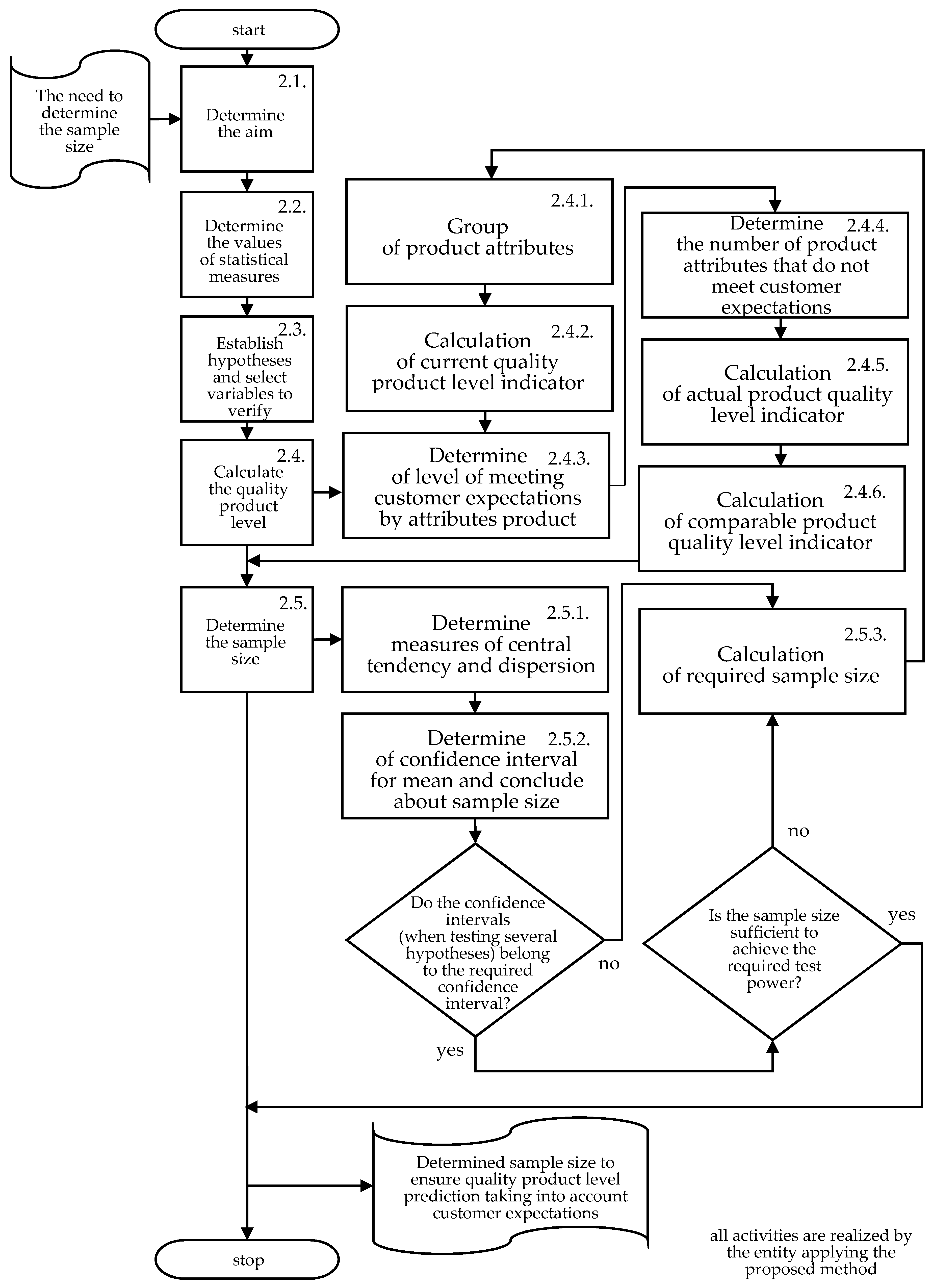
2. Methods

By referring to accepted theses, modification of the existing method of sample size determination, in which the mean value of the general population (i.e., arithmetic mean of the sample) is calculated, was undertaken [48,49]. This was because the estimator met the attributes required to determine the sample size, i.e., compliant, unbiased, effective, and sufficient [48]. The modification of the method of sample size determination considered a number of factors, namely, universal hypotheses, the method of choosing variables, and determination of the relationships of these variables to verify hypotheses. Then, the method to determine the product’s quality level was used, namely, the alternative-punctual (MAP) method. The product quality level determined in this manner was then included in the method of sample size determination. Additionally, modification consisted of simultaneously determining the sample size to test a number of hypotheses, provide a test power for this sample size, and to detect statistically significant differences for several relationships between the sample size and the test power. This approach allows the determination of the customer sample size required to predict a product’s quality level, taking into account customer expectations. Thus, it was possible to determine the number of customers from whom expectations should be obtained and processed, to allow the product’s quality level to be predicted, for which this prediction is realized based on actual and modified product quality level. The proposed method of sample size determination includes five main stages (Figure 1).

2.1. Determine the Aim

The first step is to determine the aim of the entity applying the proposed method. The aim should be determined as part of the calculation of the sample size to predict the product quality level taking into account customers’ expectations. Furthermore, the aim should include the possibility of simultaneously determining the sample size to test hypotheses, provide a test power for the sample size, and to detect a statistically significant difference for several relationships between the sample size and the test power. In this case, relationships are understood to exist between the current product quality level and the level resulting from the modified attributes of the product. In this process, it was necessary to use the SMART method, which is illustrated in the relevant literature, e.g., [50].

2.2. Determine the Values of Statistical Measures

The second step is to determine the selected statistical measures. These measures are determined by the entity applying the proposed method. According to authors of previous research [17,18,19,20,21,22,23], it was assumed that it is necessary to determine the values of the following statistical measures:

• The significance level (α) (the probability of making a type I error);
• The probability of making a type II error (β);
• The power of the statistical test (µ = 1 − β);
• The accuracy of analysis results (the so-called error of respect) (d).

The indicated statistical measures are used to verify research hypotheses, about which two types of errors may be made. The probabilities of these errors are represented as α and β [20]. The significance level (α), i.e., the probability of making a type I error (α), refers to the incorrect confirmation of an alternative hypothesis (i.e., H₁) [18,22,23]. By comparison, the probability of making a type II error (β) refers to the detection efficiency of the incorrect alternative hypothesis (H₁), for which negation is the null hypothesis (i.e., H₀) [18]. Recognizing that the null hypothesis is unlikely provides the basis for adopting an alternative hypothesis, which is the intention of the process of statistical hypothesis verification [18]. This process of verification of statistical hypotheses, in which the null hypothesis is the opposite of the alternative hypothesis, is considered to be reject-confirmatory testing (OP) [20]. This decision making is presented in

Table 1. Making decisions while verifying hypotheses. Own study based on [18].

		Hypothesis—Probability
		H0	H1
Decision about choice of hypothesis	H0	Correct acceptance H0 1-β	Type II error β
	H1	Type I error α	Correct rejection H0 1- α

.

Therefore, the entity applying the proposed method first determines the significance level (α). It is possible to set the significance level equal to 0.10, 0.05, 0.01, or 0.001 [18], and the choice is dependent on the entity applying the method. The lower the significance level, the more difficult it is to reject the null hypothesis (H₀). Therefore, a significance level equal to 0.01 or 0.001 is preferred for demanding analysis, e.g., in medical research [17,18]. As indicated by the authors of works [17,18,21,22], a significance level of α = 0.05 is preferred because this value represents a compromise between the possibilities of error and the effectiveness of applying statistical testing.

The entity applying the method then determines the probability of making a type II error (β) and the power of the statistical test (µ = 1 − β), which refers to the test’s ability (in terms of probability) to identify an incorrect null hypothesis (H₀) when it is actually unlikely [19,23]. It is assumed that a large difference between the value in the null hypothesis (H₀) and the postulated value in the alternative hypothesis (H₁) increases the test power compared to the case of small differences [18]. Because statistical tests are significance tests in practice, and do not control the probability of a type II error (β), this probably should not be high. Because the minimum power of the statistical test is µ ≥ 0.8 [20,21,23], the probability of a type II error (β) should be determined to be β ≥ 0.2 (which results from the dependence: µ = 1 − β) [18,20,23].

The entity applying the proposed method then determines the accuracy of the analysis results (the so-called error of respect) based on previous research [18,51]. In this case, the accuracy of the product quality level (actual and modified) and the accuracy of the assessment of the product’s attributes are determined a priori.

Subsequently, for the adopted values of the statistical measures, statistical tables are necessary to determine [17,52,53]:

• The confidence level (p = α − 1);
• The critical values of the normal standardized distribution (_αu);
• t-statistics with Student’s t-distribution and n-1 degrees of freedom (_αt);

which, as indicated in previous research [17,18,19,20,21], are necessary to determine the sample size.

Based on the values of these statistical measures it is possible to verify the accepted theses. Following the determination of the values of these statistical measures, the next step of the proposed method can be undertaken.

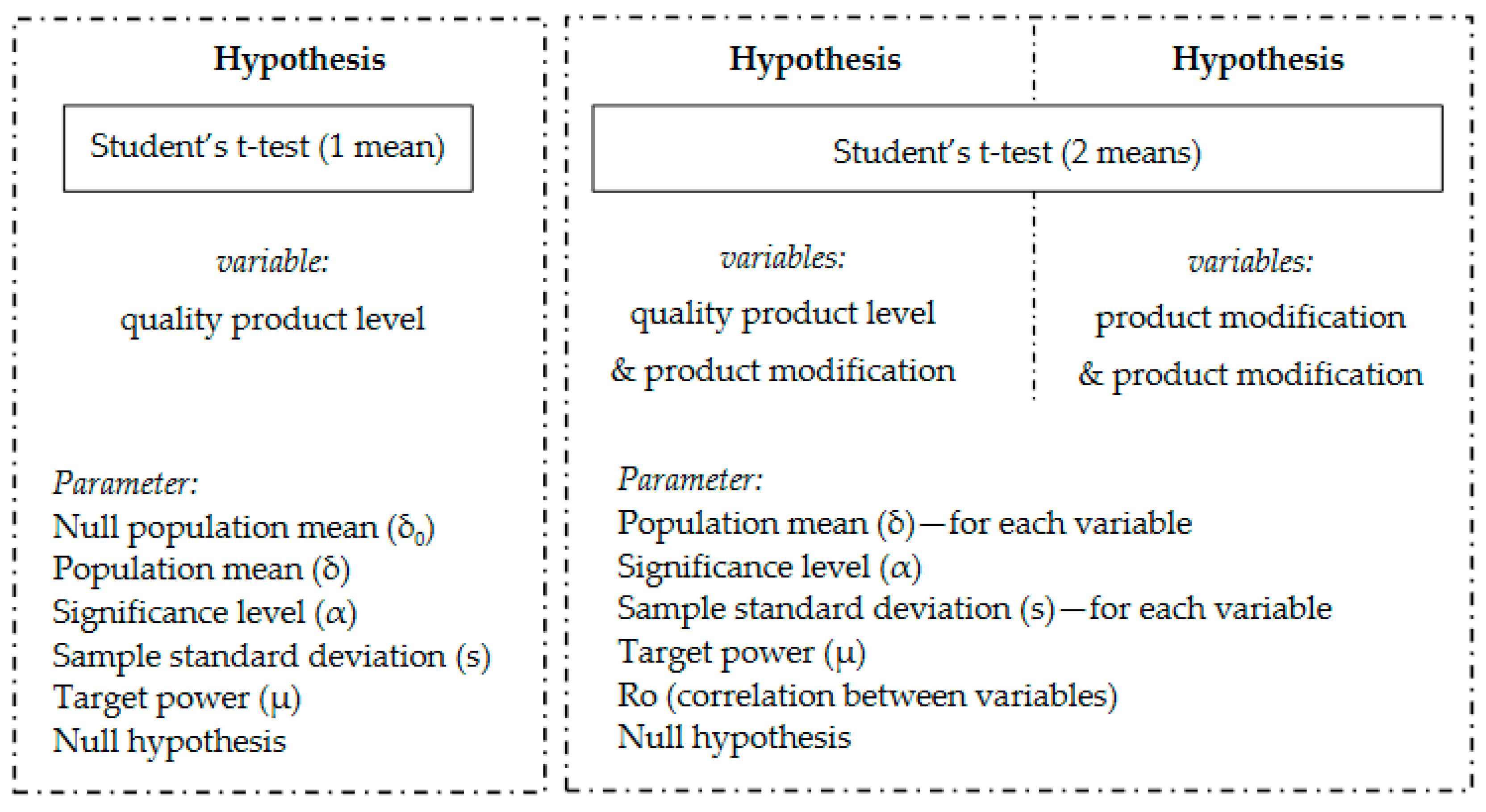
2.3. Establish Hypotheses and Select Variables to Verify Hypotheses

The third step of the proposed method is to establish research hypotheses and variables to verify these hypotheses. The hypotheses are established by the entity applying the method in the context of the aim of the research [18,20]. Based on this aim, the current authors propose the adoption of three alternative hypotheses and their opposite hypotheses.

The first hypothesis refers to the detection of statistically significant differences in product quality level depending on its modification:

• H₀: There is no difference in the quality product level when the product is modified.
• H₁: There is a difference in the quality product level when the product is modified.

The second hypothesis refers to the detection of statistically significant differences in the case of customers’ assessments of product modification:

• H₀: There is no difference in the evaluation of product modification.
• H₁: There is a difference in the evaluation of product modification.

As part of the third hypothesis, it is proposed to verify the statistically significant difference between the number of observations available to the entity applying the method at a given moment, and the number of observations required to obtain the product quality level with the accepted accuracy as part of ensuring the required test power:

• H₀: There is no difference in the actual and required number of observations to ensure the accepted accuracy of the product quality level and the test power.
• H₁: There is a difference in the actual and required number of observations to ensure the accepted accuracy of the product quality level and the test power.

It was assumed that the proposed hypotheses would allow for the verification of statistically significant differences and the prediction of the level of a product’s quality, taking into account customer expectations. However, these hypotheses are not a rule and can be modified depending on the needs of the entity applying the proposed method. Subsequently, based on the constructed hypotheses, the entity applying the proposed method chooses the number and type of variables to ensure the research hypotheses can be verified; for example, the choice of variables is characterized in the article [54]. This applies to the determination of independent (explanatory) variables and dependent (explained) variables. The independent variables are those that are controlled and that may influence dependent variables. By compaison, the dependent variables are those whose values are measured [54]. In the analysed context, the dependent variable is the product quality level, and the independent variables are those relating to product modification. Based on the established research hypotheses and the selected variables, the next stage of the proposed method can be implemented.

2.4. Calculate the Quality Product Level

The fourth stage of the method is to calculate the product quality level. The product quality level can be calculated by any appropriate method; commonly used methods include Quality Function Deployment (QFD) [33,34,35,36], integrated Fuzzy Analytical Hierarchy Process (FAHP) and quality–cost analysis [55], the Formalized Punctation (PS) method [56], or the alternative-point method (the MAP method, also called the Czechowski method) [57,58,59]. The choice of method to calculate the product quality level depends on the entity applying the proposed method. As part of the test of the method for determining the sample size, it is proposed to use the uncomplicated MAP method (Czechowski’s method), which has been applied to calculate the product quality level, taking into account the importance of the criteria [57,58,59]. The process of calculating the product quality level using the MAP method is presented in six steps.

2.4.1. Group of Product Attributes

The first step is to group all of the product attributes selected by the entity applying the method to determine the quality product level. Any number of attributes of the product can be chosen, during brainstorming (BM) or by using the multiple-voting technique, as shown in [47]. Then, to group product attributes, it is necessary to make assessments of the importance of these attributes. This assessment can be done in a subjective manner by the entity applying the method (i.e., experts) [57,58]. However, in the context of determining the product quality level taking into account customers’ expectations, the importance of the attributes should be determined based on customers’ assessments [4,5,6]. To achieve this aim, survey research can be conducted [24,25]. Assessment of the importance of product attributes can be undertaken using Saaty scales (i.e., 1–9 or 1–7) [47], the commonly used Likert scale [60], or another scale chosen by the entity applying the method. Then, the ratings provided by customers to product attributes are used to group individual product attributes according to their importance. In accordance with the MAP method, the grouping of product attributes can be performed for a group of attributes, i.e., critical (k), important (w), moderately important (s), and not very important (m). However, it is preferable to identify a group of critical attributes with a group of important attributes. This is due to the need to interpret critical attributes as being absolutely necessary [57,58].

As part of the grouped product attributes, the average value from all customer assessments is determined for each attribute (1) [17]:

$$\overline{\mathrm{x}}=\frac{{{\displaystyle \sum }}_{\mathrm{i}=1}^{\mathrm{n}}{\mathrm{x}}_{\mathrm{i}}}{\mathrm{n}}$$

(1)

where:

x_i is the value of variable for the i-th element of the general population selected for the sample,

n is sample size.

The arithmetic mean was used because it is an unbiased estimator [48,49], and has the highest reliability of the value of an expected random variable when the number of events is sufficiently large (>100) [17] or the variable distribution is normal. In the case when the entity applying the method has a small number of observations or the distribution is not normal, e.g., there are outliers, the median may provide more reliable results [49].

Then, it is possible to group the product attributes into groups: important (w), moderately important (s), and not very important (m). For this purpose, the maximum (${\overline{\mathrm{x}}}_{\max })$ and minimum (${\overline{\mathrm{x}}}_{\min })$ average values of all of the values are determined. Subsequently, the quotient of the obtained maximum and minimum values to the number of groups of attributes is calculated (2):

$$\mathrm{z}=\frac{{\overline{\mathrm{x}}}_{\max }-{\overline{\mathrm{x}}}_{\min }}{{\mathrm{n}}_{\mathrm{g}}}$$

(2)

where:

z is the value that determines the extent to which the attribute belongs to the group,

${\overline{\mathrm{x}}}_{\max }$ is the maximum rating value,

${\overline{\mathrm{x}}}_{\min }$ is the minimum rating value,

n_g is the number of attribute groups.

Then, in order to determine the range of attribute belonging to the group, the following formulas are used (3–4):

$$\begin{gathered} {\mathrm{z}}_{{\mathrm{w}}_{\mathrm{i}}}={\overline{\mathrm{x}}}_{\max }-\mathrm{z};{\mathrm{z}}_{{\mathrm{s}}_{\mathrm{i}}}={\mathrm{z}}_{{\mathrm{w}}_{\mathrm{i}}}-\mathrm{z};{\mathrm{z}}_{{\mathrm{m}}_{\mathrm{i}}}={\mathrm{z}}_{{\mathrm{s}}_{\mathrm{i}}}-\mathrm{z}; \\ \mathrm{where}:{\mathrm{z}}_{{\mathrm{m}}_{\mathrm{i}}}={\overline{\mathrm{x}}}_{\min } \end{gathered}$$

(3)

$$\begin{gathered} {\mathrm{z}}_{\mathrm{w}}\in \langle {\overline{\mathrm{x}}}_{\max };{\mathrm{z}}_{{\mathrm{w}}_{\mathrm{i}}}\rangle \\ {\mathrm{z}}_{\mathrm{s}}\in ({\mathrm{z}}_{{\mathrm{w}}_{\mathrm{i}}};{\mathrm{z}}_{{\mathrm{s}}_{\mathrm{i}}}> \\ {\mathrm{z}}_{\mathrm{m}}\in ({\mathrm{z}}_{{\mathrm{s}}_{\mathrm{i}}};{\mathrm{z}}_{{\mathrm{m}}_{\mathrm{i}}}> \end{gathered}$$

(4)

where:

${\mathrm{z}}_{{\mathrm{w}}_{\mathrm{i}}}$ is the value determining the extent to which the attributes belong to important groups,

${\mathrm{z}}_{{\mathrm{s}}_{\mathrm{i}}}$ is the value determining the extent to which the attributes belong to moderately important groups,

${\mathrm{z}}_{{\mathrm{m}}_{\mathrm{i}}}$ is the value determining the extent to which the attributes belong to not very important groups,

z, ${\overline{\mathrm{x}}}_{\max }$ and ${\overline{\mathrm{x}}}_{\min }$ is as above,

z_w is the scope of belonging of attributes of important groups,

z_s is the scope of belonging of attributes of moderately important groups,

z_m is the scope of belonging of attributes of not very important groups.

After determining the scope of belonging (z_w, z_s, z_m), the attributes of the product are grouped. Then, the number of product attributes in the groups is determined, taking into account fixed attribute weights according to the MAP method, i.e., 50:10:1 for important, moderately important, and not very important, respectively.

2.4.2. Calculation of Current Quality Product Level Indicator

The second step is the calculation of the current quality product level indicator (Qo). This indicator is calculated by the entity applying the method for each observation (i.e., for assessments by each customer). The indicator Qo refers to the situation in which the product attributes fully meet the customer’s expectations. According to the authors of works [57,58], the indicator of the current product quality level is determined by Formula (5):

$${\mathrm{Q}}_{\mathrm{o}}=50{\mathrm{n}}_{\mathrm{w}}+10{\mathrm{n}}_{\mathrm{s}}+1{\mathrm{n}}_{\mathrm{m}}$$

(5)

where:

n_w is the number of product attributes in the important group;

n_s is the number of product attributes in the moderately important group;

n_m is the number of product attributes in the not very important group;

50; 10; 1 is fixed attribute weights according to the MAP method.

After calculating the indicator of the current product quality level, it is possible to perform the next step of the method.

2.4.3. Determine of Level of Meeting Customer Expectations by Product Attributes

The third step is to determine the level of meeting customer expectations by product attribute (q_s). This level is determined by the entity applying the proposed method, based on the scale of meeting customer expectations by product attribute, as shown in

Table 2. Interpretation of the product quality compliance level. Own study based on [57].

Interpretation of the Product Quality Compliance Level		Numerical Range of the Quality Level
Verbal Interpretation	Numerical Interpretation
Bad	9	<0; 0.1)
Critical	8	<0.1; 0.2)
Unfavorable	7	<0.2; 0.3)
Unsatisfactory	6	<0.3; 0.4)
Sufficient	5	<0.4; 0.5)
Moderate	4	<0.5; 0.6)
Satisfactory	3	<0.6; 0.7)
Beneficial	2	<0.7; 0.8)
Distinctive	1	<0.8; 0.9)
Excellent	0	<0.9; 1>

.

According to works [57,58], the current authors propose determining the level of product quality compliance at a minimum level of 0.6, which is a satisfactory level. However, the final decision on whether the product quality level is met depends on the entity applying the method.

2.4.4. Determine the Number of Product Attributes that Do Not Meet Customer Expectations

The fourth step is to determine the number of product attributes that do not meet customers’ expectations [57,58]. The cardinality is determined by the entity applying the proposed method for each observation (i.e., for assessments by each customer). The cardinality is determined based on the level of product quality compliance (Section 2.4.3). The number of product attributes that do not meet customer expectations should be categorized into groups of product attributes (important, moderately important, not very important). Then, the entity applying the method (for each attribute of the product) compares the current product quality indicator (Q_o) (calculated in Section 2.4.2) with the level of product quality compliance (q_s) (Section 2.4.3), using Dependence (6):

$$\begin{array}{cc}\mathrm{if} {\mathrm{Q}}_{\mathrm{o}}\ge {\mathrm{q}}_{\mathrm{s}}\hfill & \hfill \mathrm{product} \mathrm{attribute} \mathrm{meets} \mathrm{the} \mathrm{customer} \mathrm{expectations} \mathrm{and} \in ({\mathrm{m}}_{\mathrm{w}};{\mathrm{m}}_{\mathrm{s}};{\mathrm{m}}_{\mathrm{m}})\hfill \\ \mathrm{if} {\mathrm{Q}}_{\mathrm{o}}<{\mathrm{q}}_{\mathrm{s}}\hfill & \hfill \mathrm{product} \mathrm{attribute} \mathrm{does} \mathrm{not} \mathrm{meets} \mathrm{the} \mathrm{customer} \mathrm{expectations} \mathrm{and} \in ({\mathrm{m}}_{\mathrm{w}};{\mathrm{m}}_{\mathrm{s}};{\mathrm{m}}_{\mathrm{m}})\hfill \end{array}$$

(6)

where:

Q₀ is the indicator of current quality product level;

q_s is the level of product quality compliance;

m_w is the number of important product attributes that the product does not meet;

m_s is the number of moderately important product attributes that the product does not meet;

m_m is the number of not very important product attributes that the product does not meet.

Then, it is possible to carry out the next step of the method.

2.4.5. Calculation of Actual Product Quality Level Indicator

The fifth step is the calculation of the actual product quality level indicator (Q_i), which is the indicator that includes the attributes that do not meet customer expectations [57,58]. This indicator is calculated by the entity applying the proposed method for each observation (i.e., for assessments by each customer). According to authors of works [57,58], it is necessary to use Formula (7):

$${\mathrm{Q}}_{\mathrm{i}}=50\left({\mathrm{n}}_{\mathrm{w}}-{\mathrm{m}}_{\mathrm{w}}\right)+10\left({\mathrm{n}}_{\mathrm{s}}-{\mathrm{m}}_{\mathrm{s}}\right)+\left({\mathrm{n}}_{\mathrm{m}}-{\mathrm{m}}_{\mathrm{m}}\right)$$

(7)

where:

n_w is the number of product attributes in the important group;

n_s is the number of product attributes in the moderately important group;

n_m is the number of product attributes in the not very important group;

m_w is the number of important product attributes that the product does not meet;

m_s is the number of moderately important product attributes that the product does not meet;

m_m is the number of not very important product attributes that the product does not meet;

50; 10; 1 is fixed attribute weights according to the MAP method.

After calculating the actual product quality level indicator, it is possible to perform the next step.

2.4.6. Calculation of Comparable Product Quality Level Indicator

The sixth step of the method is the calculation of the comparable product quality level indicator (q_i) [57,58]. This indicator is calculated by the entity applying the proposed method using Formula (8), i.e., the quotient of the actual product quality level indicator (Q_i) and the current quality product level indicator (Q_o) [57,58]:

$${\mathrm{q}}_{\mathrm{i}}=\frac{{\mathrm{Q}}_{\mathrm{i}}}{{\mathrm{Q}}_{\mathrm{o}}}$$

(8)

where:

Q_i is the actual product quality level indicator;

Q_o is the current quality product level indicator.

The comparable product quality level indicator is calculated for each observation (i.e., for assessments by each customer). In accordance with the assumptions of the MAP method, the q_i indicator has values with the range 0 ≤ q_i ≤ 1 [57,58]. If the resulting value q_i does not fall within the range 0 ≤ q_i ≤ 1, the process of quality product level determination should be repeated from Section 2.4.1. The process should be repeated until the calculations are correct.

The values of q_i represent the product quality level required by customers. Interpretation of this indicator is shown in Table 2 (in Section 2.4.3). Therefore, based on values of the q_i indicator, the minimum value of the sample size to predict the product quality level, taking into account customers’ expectations, was assumed.

2.5. Determine the Sample Size

The fifth stage is to determine the research sample size that allows the prediction of the product quality level taking into account customers’ expectations. Following the authors of works [17,18,61], it was necessary to determine selected values of measure of central tendency, spread, and confidence interval. Additionally, as part of the method, the process of determining the sample size was modified. The process of calculating the sample size is presented using both a traditional approach (mathematical equations) and Statistica 13.3. This stage is presented in three steps.

2.5.1. Determine Measures of Central Tendency and Dispersion

The first step for the entity applying the proposed method is to determine the selected measures of central tendency and dispersion. The values necessary to calculate the sample size are [17,18,61]:

• The current sample size (n);
• The sample mean ($\overline{\mathrm{x}}$);
• The sample variance (s²);
• The sample standard deviation (s).

These measures of central tendency and dispersion are characterized in the literature, e.g., [17].

The current sample size (n) represents the number of samples available to the entity applying the method, at the time of determining the sample size, to predict the product quality level taking into account customer expectations.

Then, the entity calculates for each variable (selected in Section 2.3) the sample mean $\left(\overline{\mathrm{x}}\right)$ using Formula (9) [17]:

$$\mathrm{x}¯=\frac{{{\displaystyle \sum }}_{\mathrm{i}=1}^{\mathrm{n}}{\mathrm{x}}_{\mathrm{i}}}{\mathrm{n}}$$

(9)

where:

x_i is the value of variable for the i-th element of the general population selected for the sample;

n is sample size.

Then, the entity applying the method calculates for each variable (selected in Section 2.3) the sample variance (s²) using Formula (10) [17]:

$${\mathrm{s}}^2=\frac{{{\displaystyle \sum }}_{\mathrm{i}=1}^{\mathrm{n}}{\left({\mathrm{x}}_{\mathrm{i}}-\overline{\mathrm{x}}\right)}^2}{\mathrm{n}-1}$$

(10)

where:

x_i is the value of variable for the i-th element of the general population selected for the sample;

$\overline{\mathrm{x}}$ is the sample mean;

n is the current sample size.

Then, it is possible to calculate the sample standard deviation (s) for each variable selected in Section 2.3. The sample standard deviation (s) is calculated by the entity applying method using Formula (11) [17]:

$$\mathrm{s}=\sqrt{{\mathrm{s}}^2}$$

(11)

where:

s² is the sample variance.

The indicated values can be calculated using Statistica 13.3. (via basic statistics or descriptive statistics) [18,20]. Then, it is possible to perform the next step of the method.

2.5.2. Determine the Confidence Interval for Mean and Determine the Sample Size

The second step is to determine the confidence interval (CI) for the mean and reach a conclusion about the sample size. The confidence interval is a statistic used to determine the true result with an assumed probability [61]. The confidence interval is determined for each variable selected in Section 2.3 to calculate the unknown parameters of the population with an assumed probability, i.e., the confidence level (p = 1 − α) (assumed in Section 2.2). The confidence interval is determined for the mean value resulting from the method, which was used to modify part of the calculation of the estimator of the mean value of the general population (i.e., the arithmetic mean of the sample) [48,49]. In the case in which the mean of the population is unknown, by assuming that the sample size is large, i.e., n > 100 [17,21], the confidence interval can be determined be taking into account the sample standard deviation (12) [17]:

$$\overline{\mathrm{x}}-\frac{{}_{\propto }\mathrm{u}\times \mathrm{s}}{\sqrt{\mathrm{n}}}<\mathsf{\mu }<\overline{\mathrm{x}}+\frac{{}_{\propto }\mathrm{u}\times \mathrm{s}}{\sqrt{\mathrm{n}}}$$

(12)

where:

$\overline{\mathrm{x}}$ is the sample mean (calculated in Section 2.5.1);

s is the sample standard deviation (calculated in Section 2.5.1);

_αu is the critical values to normal standardized distribution (determined in Section 2.2);

n is the sample size (determined in Section 2.5.1).

Subsequently, the entity applying the method can make a decision about the sample size. The entity thus considers whether the current research sample size has ensured the accuracy of the analysis results (d) for the assumed significance level (α).

Following [17], it was assumed that the required range of the confidence interval is determined as (13):

$$\mathsf{\mu }=2\mathrm{d}$$

(13)

where:

µ is the span of confidence interval;

d is the accuracy of analysis results (d) (determined in Section 2.2).

Because the range of the confidence interval is determined for each variable selected in Section 2.3, it was considered that inference should be undertaken for two cases:

Case 1. When at least one of the determined confidence intervals (as part of testing several hypotheses) does not belong to the required confidence interval, then it is necessary to determine the number of additional observations (n_d) required in the sample to achieve the desired test power.

Case 2. When all of the determined confidence intervals (as part of testing several hypotheses) belong to the required confidence interval, then it is necessary to determine (as part of testing research hypotheses), whether the current sample size will achieve the assumed test power.

The applications of these cases are shown in the next step of the method.

2.5.3. Calculation of Required Sample Size

The third step is to calculate the required sample size to predict the product quality level taking into account customers’ expectations. To test the method, two techniques are proposed to calculate the required sample size, i.e., the traditional approach (mathematical equations) or using the tools of Statistica 13.3. This step is performed by the entity applying the method as appropriate for case 1 or case 2.

Procedure for the Occurrence of the First Case:

If the entity concludes that at least one of the determined confidence intervals (as part of testing several hypotheses) does not belong to the required confidence interval, then it is necessary to present the confidence interval as a sample size function [17], for which the confidence interval and accuracy are calculated from Formulas (14) and (15). Furthermore, the required number of observations in sample n₀ that results in a confidence interval that is not greater than an assumed range equal to 2d, is determined from Formula (16) [17]:

$$\overline{\mathrm{x}}-\mathrm{d}<\mathsf{\mu }<\overline{\mathrm{x}}-\mathrm{d}$$

(14)

$$\mathrm{d}={}_{\propto }\mathrm{t}\frac{\mathrm{s}}{\sqrt{\mathrm{n}}}$$

(15)

$${\mathrm{n}}_0=\frac{{}_{\propto }\mathrm{t}{}_{ }^2{\mathrm{s}}^2}{{\mathrm{d}}^2}$$

(16)

where:

µ is the span of confidence interval;

$\overline{\mathrm{x}}$ is the sample mean (calculated in Section 2.5.1);

d is the accuracy of analysis results (d) (determined in Section 2.2);

_αt is t-statistics with Student’s t-distribution and n-1 degrees of freedom (determined in Section 2.2);

s is the sample standard deviation (calculated in Section 2.5.1);

n is the sample size (determined in Section 2.5.1);

n₀ is the required number of observations in sample.

After determining the required number of observations in the sample (n₀), which is not greater than the current sample size (n), it is possible to determine the additional number of observations in the sample (17) [17]:

$${\mathrm{n}}_{\mathrm{d}}={\mathrm{n}}_0-\mathrm{n}$$

(17)

where:

n_d is the number of additional observations in the sample;

n₀ is the required number of observations in the sample (calculated according to Formula 16);

n is the sample size (determined in Section 2.5.1).

Then, it is possible to check if the number of observations in the sample achieves the desired test power. For this purpose, it is proposed to use computer tools, i.e., Statistica 13.3. [18,20], as shown in the next section.

Procedure for the Occurrence of the Second Case:

If the entity applying the method concludes that all of the determined confidence intervals (as part of testing several hypotheses) belong to the required confidence interval, then it is necessary to determine (as part of testing research hypotheses) whether the current sample size (n₀) can achieve the assumed test power. For this case, the advanced and multidimensional tools of Statistica are used, i.e., test power analysis [18,20]. In the context of research about the determination of sample size (adopting the three hypotheses presented in Section 2.3), Student’s t-test is commonly applied for one and two means, separately [21,54,62]. For this purpose, it is necessary to determine the parameters shown in Figure 2.

The measure of the population mean (δ) refers to the accuracy of the analysis results (i.e., estimation error of the analyzed value compared the real value), and requires calculation of the potential difference between the average value and the actual value. The measure of population mean (δ) is determined by Formula (18) [18]:

$$\mathsf{\delta }=\pm \mathrm{d}\overline{\mathrm{x}}$$

(18)

where:

δ is the population mean;

d is the accuracy of analysis results;

$\overline{\mathrm{x}}$ is the sample mean for the variable.

In the context of determining the null population mean (δ₀) and the null hypothesis, following [18], the following hypotheses were assumed: H₀: δ₀ = 0 and H₁: δ₀ ≠ 0, wherein the null population mean has value δ₀ = 0. Following [17], it was also assumed that the null hypothesis is a two-sided hypothesis (H₀ = H₁). This assumption was based on the following hypotheses:

• Student’s t-test for one mean: H₀: δ = δ₀ and H₁: δ ≠ δ₀;
• Student’s t-test for two means, dependent samples: H₀: δ₁ = δ₂ and H₁: δ₁ ≠ δ₂;

where:

• δ, δ₁, δ₂ is the population mean;
• δ₀ is the null population mean.

The value of correlation can be determined using the tools of Statistica 13.3. (via basic statistical–correlation matrices). The significance level (α) and target power are the same as the measures determined in Section 2.2, and the sample standard deviation (s) was calculated in Section 2.5.1. After determining the values of all measures, it is necessary to enter these values into Statistica 13.3. (in: test power analysis), initiate a test run, and estimate the required sample size.

The number of determined sample sizes, taking into account the achievement of the required test power, is equal to the number of defined research hypotheses. First, it is necessary to verify that, given the power of the statistical test, the current sample size is greater than or equal to each of the sample sizes that were calculated as part of the hypothesis verification:

• If the current sample size is greater or equal to each of the obtained sample sizes, it can be concluded that the current sample size achieves the assumed test power for verifying the research hypotheses. This sample size is sufficient to predict the product quality level taking into account customers’ expectations; thus, the process of determination of the sample size can be stopped (19) [17]:

  $$\mathrm{n}={\mathrm{n}}_0$$

  (19)

  where:
  n is the current sample size;
  n₀ is the required number of observations in sample.
• If the current sample size is less than at least one of the obtained sample sizes, it can be concluded that current sample size does not allow the assumed test power to be to achieved for verifying the research hypotheses. Then, the required sample size (n₀) that allows the established research hypotheses to be verified is the maximum sample size (n_max) among all of those analyzed (20):

  $${\mathrm{n}}_0={\mathrm{n}}_{\max },\mathrm{where}{\mathrm{n}}_{\max }\in \left\{\mathrm{n},{\mathrm{n}}_1,{\mathrm{n}}_2,\dots ,{\mathrm{n}}_{\mathrm{n}}\right\}$$

  (20)

  where:
  n₀ is the required number of observations in sample;
  n_max is the maximum sample size among all sample sizes;
  n is the current sample size;
  n_1, n₂,…, n_n is the required sample size as part of the verification of the adopted research hypotheses.

The determination that the required sample size is the largest sample size among all of those analyzed is confirmed by the fact that, as the sample size increases, the power of the test increases [18]. The process ends when all assumptions of the method are met and the sample size is sufficiently large.

3. Results

The method to determine the sample size was modified for this research, which concerns the prediction of a product’s quality level, taking into account customers’ expectations. In this research, the predicted product quality level is estimated based on the current and modified product quality, and the customers are buyers or potential buyers of the product. To account for customers’ expectations, following [24,25,36], survey research was undertaken to obtain the assessments of the importance of the product attributes, and the current and modified product quality level. To determine the current level of the product quality, the customers in the survey assess the product in its existing physical state (i.e., selected product attributes) using a Likert scale [60]. When determining the levels resulting from product modification (i.e., modification of selected product attributes), again using the Likert scale [60], the surveyed customers assess the proposed changes in the product attributes. The aim of distinguishing between the attributes of the current and modified products is to predict the product’s quality level and to ensure that it satisfies the customers’ expectations. To determine the level of product attributes at which the customers’ expectations were satisfied, the preferred Kolman scale was adopted (Table 2) [57,58]. Following [57,58], a value of 0.6 was assumed as the boundary at which the satisfactory and unsatisfactory levels of the product’s quality could be determined. The range of <1; 0.6> represents the satisfactory level, comprising the levels of moderate, satisfactory, beneficial, distinctive, and excellent. Furthermore, the unsatisfactory product quality level refers to the range (0.6; 0>, and comprises the levels sufficient, unsatisfactory, unfavorable, critical, and bad. To determine product quality levels, statistical tests using Statistica 13.3 were carried out, and the uncomplicated MAP method was used [57,58,59], which allowed the importance of product attributes to be included. This made it necessary to determine the size of the research sample. For this purpose, the modified method to determine the research sample size presented in this article was developed. When testing the proposed method, a research sample of n = 157 customers was used. Based on the method and following [17,18,20,21,22,51,52,53], the statistical measures noted previously were estimated. The statistical measures used in the research are shown in

Table 3. Estimated statistical measures.

Mark	Statistical Measure	Value
α	the significance level (α) (the probability of making a type I error)	0.05
α − 1	the confidence interval	0.95
αu	the critical value to normal standardized distribution which meets the condition: $P\left\{-{}_{\propto }u<{}_{\propto }u\right\}=1-\propto$	1.960
αt	value of t-statistics with t-Student distribution and n-1 degrees of freedom	1.960
d1	the accuracy (so-called error of respect) for quality product level	0.05
d2	the accuracy (so-called error of respect) for assessments product attributes	0.5
β	the probability of making a type II error	≤0.2
µ = 1 − β	the power of statistical test	≥0.8

.

Then, the research hypotheses and variables for testing these hypotheses were assumed (as shown in Section 2.3). Then, in accordance with Section 2.4, the product quality level was calculated using the MAP method [57,58,59]. First, to determine the product quality level, all attributes of the product were grouped. Twenty-two product attributes were used to calculate the product quality level. For this purpose, the arithmetic mean value of all customers’ assessments was calculated using Formula (1) for each analyzed product attribute (

Table 4. The mean values of the assessments of product attributes.

Attribute	A1	A2	A3	A4	A5	A6	A7	A8	A9	A10	A11
$\overline{x}$	4.07	4.04	4.21	3.73	4.13	2.89	3.40	3.68	3.79	3.27	3.10
Attribute	A12	A13	A14	A15	A16	A17	A18	A19	A20	A21	A22
$\overline{x}$	2.45	2.99	3.20	3.35	2.86	2.62	3.78	3.47	3.75	4.06	2.66

).

Then, the maximum (${\overline{\mathrm{x}}}_{\max })$ and minimum (${\overline{\mathrm{x}}}_{\min })$ mean values from all obtained values were determined, where ${\overline{\mathrm{x}}}_{\max }$ = 4.21 and ${\overline{\mathrm{x}}}_{\min }$ = 2.45. Next, the quotient of the obtained maximum and minimum values to the number of groups of attributes was calculated using Formulas (2) and (21):

$$\begin{gathered} \mathrm{z}=\frac{4.21-2.45}{3} \\ \mathrm{z}=0.59 \end{gathered}$$

(21)

Then, using Formulas (3) and (4) the scope of the attributes belonging to groups was determined (22)–(23):

$$\begin{gathered} {\mathrm{z}}_{{\mathrm{w}}_{\mathrm{i}}}=4.21-0.59=3.62 \\ {\mathrm{z}}_{{\mathrm{s}}_{\mathrm{i}}}=3.62-0.59=3.04 \\ {\mathrm{z}}_{{\mathrm{m}}_{\mathrm{i}}}=3.04-0.59=2.45 \end{gathered}$$

(22)

$$\begin{gathered} {\mathrm{z}}_{\mathrm{w}}\in \langle 4.21;3.62\rangle \\ {\mathrm{z}}_{\mathrm{s}}\in (3.62;3.04> \\ {\mathrm{z}}_{\mathrm{m}}\in (3.04;2.45> \end{gathered}$$

(23)

where all marks are the same as in Formulas (3) and (4).

After grouping all of the product attributes into groups (important, moderately important, and not very important), the number of these attributes in each group was determined (

Table 5. The number of product attributes in each group.

Marks and Weights of Attributes Product			the Number of Attributes in Groups
mark	description	weight	number
nw	number of product attributes in important group	50	5
ns	number of product attributes in moderately important group	10	11
nm	number of product attributes in not very important group	1	6

).

Then, using Formula (5), the current product quality level indicator (Q_o) was calculated (24):

$$\begin{gathered} {\mathrm{Q}}_{\mathrm{o}}=50\times 5+10\times 11+1\times 6 \\ {\mathrm{Q}}_{\mathrm{o}}=366 \end{gathered}$$

(24)

The indicator of the current product quality level was equal to Q_o = 366. Next, following [57,58], the level at which customer expectations by product attribute was considered to be satisfactory was set, i.e., q_s = 0.6. For this reason, based on the assumed satisfactory level (q_s = 0.6), the number of product attributes that did not meet customers’ expectations was determined (i.e., m_w, m_s, m_m, as shown in Section 2.4.4). Then, using Formulas (7) and (8), the actual product quality level (Q_i) and comparable product quality indicator were calculated (q_i). Because the calculation was performed for the sample size n = 157,

Table 6. An fragment of the obtained results.

Observation Number	mw	ms	mm	Qi	qi
1	0	2	1	345	0.94
2	1	1	0	306	0.84
3	0	0	0	366	1.00
4	0	3	0	336	0.92
5	1	4	3	273	0.75
6	0	0	1	365	1.00
7	0	0	2	364	0.99
8	0	0	1	365	1.00
9	0	2	0	346	0.95
10	1	2	2	294	0.80
157	0	0	1	365	1.00

shows only a fragment of the obtained results.

It was concluded that the calculation was correctly realized and the results were fully consistent, because the comparable product quality indicator (q_i) for each observation was in the range of the MAP method, i.e., <0; 1> [57,58]. For each variable (quality product level and two product modifications), Formulas (9)–(11) were used to calculate the values of the measures of central tendency and dispersion (

Table 7. The values of measures of central tendency and dispersion for the analyzed variables.

Measure	Quality Product Level	Modification 1	Modification 2
the sample size (n)	157	157	157
the sample mean ($\overline{\mathrm{x}})$	0.88	3.60	4.45
the sample variance (s2)	0.04	2.23	1.08
the sample standard deviation (s)	0.19	1.50	1.04

).

Then, using Formula (12) and the adopted values of statistical measures, the confidence interval was determined for each of the analyzed variables, i.e., for product quality level (25), the first modification of the product (26), and the second modification of the product (27):

$$\begin{gathered} 0.88-\frac{1.960\times 0.19}{\sqrt{157}}<\mathsf{\mu }<0.88+\frac{1.960\times 0.19}{\sqrt{157}} \\ 0.85<\mathsf{\mu }<0.91 \\ \mathrm{LL}-\mathrm{UL}=0.91-0.85=0.06 \end{gathered}$$

(25)

$$\begin{gathered} 3.60-\frac{1.960\times 1.50}{\sqrt{157}}<\mathsf{\mu }<3.60+\frac{1.960\times 1.50}{\sqrt{157}} \\ 3.37<\mathsf{\mu }<3.83 \\ \mathrm{LL}-\mathrm{UL}=3.83-3.37=0.47 \end{gathered}$$

(26)

$$\begin{gathered} 4.45-\frac{1.960\times 1.04}{\sqrt[]{157}}<\mathsf{\mu }<4.45+\frac{1.960\times 1.04}{\sqrt[]{157}} \\ 4.29<\mathsf{\mu }<4.61 \\ \mathrm{LL}-\mathrm{UL}=4.61-4.29=0.33 \end{gathered}$$

(27)

where:

LL is upper bound of the confidence interval;

UL is lower bound of the confidence interval.

Subsequently, it was determined if the current research sample size ensured the accuracy of analysis results (d) was achieved for the assumed the significance level (α). For this purpose, Formula (13) was used to calculate the range of the confidence interval for each variable. Then, it was found that each of the confidence intervals belongs to the required spread of the confidence interval (28)–(30):

$$\begin{array}{cc}\mathrm{Quality}\mathrm{product}\mathrm{level}:\hfill & \\ & \hfill \mathsf{\mu }=0.1\ge 0.06\end{array}$$

(28)

$$\begin{array}{cc}\mathrm{Modification}\mathrm{of}1\mathrm{product}:\hfill & \\ & \hfill \mathsf{\mu }=1\ge 0.47\end{array}$$

(29)

$$\begin{array}{cc}\mathrm{Modification}\mathrm{of}2\mathrm{product}:\hfill & \\ & \hfill \mathsf{\mu }=1\ge 0.33\end{array}$$

(30)

Then, it was determined that the current sample size allowed the assumed test power to be achieved. For this purpose, Statistica 13.3. and Student’s t-test (for one mean and for two means) were used. The results are shown in

Table 8. Student’s t-test for one mean—sample size.

Parameter	Quality Product Level
Null population mean (δ0)	0.00
Population mean (δ)	0.04
Standard deviation in population (σ)	0.19
Standardized effect (Es)	0.21
The probability of making a type I error (α)	0.05
Target power	0.80
Power for the required sample size	0.80
Sample size required (n0)	180.00

;

Table 9. Student’s t-test for two means—sample size.

Parameter	Quality Product Level and Modification of 1 Product	Modification of 1 Product and Modification of 2 Product
Average in population (δ1)	1.80	2.23
Average in population (δ2)	0.04	1.80
Standard deviation in population (σ1)	1.50	1.04
Standard deviation in population (σ2)	0.19	1.50
Correlation between groups	0.33	0.35
Error std. for the difference of means	1.45	1.50
Standardized effect (Es)	1.21	0.29
The probability of making a type I error (α)	0.05	0.05
The critical value of t	2.36	1.98
Target power	0.80	0.80
Power for the required sample size	0.84	0.80
Sample size required (n0)	8.00	98.00

.

As result, three different values of the sample size were obtained (i.e., n₁ = 180, n₂ = 8, n₃ = 98). Because the current sample size (n = 157) was less than one of the obtained sample sizes (i.e., n₁ = 180), it was concluded that the current sample size does not allow the adopted test power to be achieved in the verification of the research hypotheses. Therefore, using Formula (20), the required sample size (n₀) was determined based on the maximum sample size (n_max) of all of analyzed values (31):

$${\mathrm{n}}_0=180,\mathrm{where}{\mathrm{n}}_{\max }\in \left\{157;180;8;98\right\}$$

(31)

where:

n₀ is the required number of observations in the sample;

n_max is the maximum sample size of all of the analyzed values (sample sizes).

The analysis was concluded at this stage because, according to the authors of [18], as the sample size increases, the test power increases.

4. Discussion

The main determinant of an organization’s success is consideration of customers’ expectations to ensure a satisfactory level of product quality [4,5,6,63,64,65,66]. This refers to undertaking sustainable development actions, i.e., obtaining, processing, and determining the product quality level [6,11,12]. In this manner, it is possible to improve, for example, current products, and to predict their quality level, taking into account customer satisfaction [5,14,67]. Realization of these actions in an effective manner is problematic in, for example, plan and control processes [11] in series production, in which it is necessary to analyze and simultaneously include different expectations and preferences of a large number of customers [9]. Therefore, the aim of the article was to propose a method to determine the research sample size to predict the product quality level, taking into account current customer expectations. This method resulted from the modification of the method for determining the size of the research sample. After testing of the method, the validity of the adopted research theses was confirmed.

Therefore, the main predicted benefits of the proposed method are as follows:

• Determination of the number of customers as part of assessing customers’ expectations about the product quality level, which may be obtained by any method, e.g., survey, questionnaire, interview [24,25];
• Processing of obtained expectations by any method (for example, the MAP method) [57,58,59] to determine the number of customers required to predict the product quality level based on the current and modified product quality levels;
• Determination of the number of customers to test research hypotheses as part of the prediction of the product quality level (as shown in Section 2.3);
• Determination of the number of customers while ensuring the test power for this sample size, and detection of statistically significant differences between several relationships for this sample size and test power, as shown in Section 2.3, i.e., product quality level, the modified product, and two different product modifications;
• Use of the method in the context of predicting customers’ expectations about the quality of any product.

In the context of series production mentioned above, an advantage is the identification of possible solutions relating to existing products, thus adapting and predicting product quality while taking into account customer expectations. Then, these organizations can gain a competitive advantage as part of fulfilling the assessed expectations using their production capabilities [2,13], which can be implemented at the product design stage [2,6,7,14]. This procedure not only results in higher satisfaction among customers, and improved economic results, but also leads to the effective implementation of sustainable development. Another advantage of the proposed method for the entity concerned is the possibility of alternative use of mathematical formulas or Statistica 13.3 to determine the sample size. The choice of technique to determine the sample size is open and depends on the preference of the individual entity. Additionally, the method has business implications, e.g., is a low costed tool for supporting preparatory activities of organizations as part of improving quality of product, by which it is possible in advance to determine the number of customers, who will be allowed to precisely determine satisfactory changes of product design. Nonetheless, a limitation of the proposed, modified method is that it refers to a situation in which the entity has an initial research sample (of any size) [48,49].

As part of subsequent research, it is planned to extend the proposed modified method to include the process of selecting customers to determine the sample size as part of the prediction of the product quality level while taking into account customer expectations. In addition, future studies will examine the prediction of the product quality level taking into account customer expectations.

5. Conclusions

A key trend in the production is customer-oriented product development. This refers to undertaking actions that take into account customers’ expectations about products. These actions include determining the number of customers from whom it is necessary to obtain expectations, and then obtaining and processing these expectations. In addition, an advantage is gained by those organizations that apply various solutions to already existing products, thus adapting these products to enhance their quality. Among other factors, this relates to the prediction of the product’s quality level. However, as shown in this paper, a single consistent method is lacking for the determination of the number of customers from whom expectations should be obtained, for processing and subsequent prediction of the product quality level. Therefore, the aim of the article was to propose a method to determine the research sample size required to predict the product quality level while taking into account current customer expectations. This approach resulted from modification of the method for determining the size of the research sample, helping organizations to achieve sustainable development and maximize product quality. Testing of the method was conducted as part of the research, in which the prediction of product quality was made on the basis of the current and modified product quality. This testing showed that the proposed method allows determination of the sample size to predict the product quality level, taking into account customer expectations about current and modified quality levels. It was shown, that in the proposed approach the sample size should be equal to 180 customers. It was also shown that this method allows prediction of the product quality level as part of the testing of a few, selected hypotheses, simultaneously provided a test power for this sample size, and detected the statistically significant differences between the relationships of several indicated variables and the specified sample size and test power. The application of the proposed method can be an effective part of the sustainable development of products. Thus, different solutions for existing products can be identified, allowing their quality to be predicted while taking into account customer expectations.

References

- Alt, R.; Ehmke, J.F.; Haux, R.; Henke, T.; Mattfeld, D.C.; Oberweis, A.; Paech, B.; Winter, A. Towards customer-induced service orchestration-requirements for the next step of customer orientation. Electron. Mark. 2019, 29, 79–91. [Google Scholar] [CrossRef]
- Zheng, P.; Xu, X.; Xie, S.Q. A weighted interval rough number based method to determine relative importance ratings of customer requirements in QFD product planning. J. Intell. Manuf. 2019, 30, 3–16. [Google Scholar] [CrossRef]
- Wang, P.; Gong, Y.; Xie, H.; Liu, Y.; Nee, A.Y. Applying CBR to machine tool product configuration design oriented to customer requirements. Chin. J. Mech. Eng. 2017, 30, 60–76. [Google Scholar] [CrossRef]
- Ostasz, G.; Czerwińska, K.; Pacana, A. Quality management of aluminum pistons with the use of quality control points. Manag. Syst. Eng. 2020, 28, 771–773. [Google Scholar] [CrossRef]
- Liu, C.; Ramirez-Serrano, A.; Yin, G. An optimum design selection approach for product customization development. J. Intell. Manuf. 2010, 23, 1433–1443. [Google Scholar] [CrossRef]
- Huang, H.-Z.; Li, Y.; Liu, W.; Liu, Y.; Wang, Z. Evaluation and decision of products conceptual design schemes based on customer requirements. J. Mech. Sci. Technol. 2011, 25, 2413–2425. [Google Scholar] [CrossRef]
- Stylidis, K.; Rossi, M.; Wickman, C.; Söderberg, R. The Communication Strategies and Customer’s Requirements Definition at the Early Design Stages: An Empirical Study on Italian Luxury Automotive Brands. Procedia CIRP 2016, 50, 553–558. [Google Scholar] [CrossRef]
- Madzik, P.; Chocholakova, A. Structured Transfer of Customer’s Requirements into Product Quality Attributes-A University Case Study. Qual. Access Success 2016, 17, 38–45. [Google Scholar]
- Pacana, A.; Pasternak-Malicka, M.; Zawada, M.; Radon-Cholewa, A. Decision support in the production of packaging films by cost-quality analysis. Przemysł Chem. 2016, 95, 1042–1044. [Google Scholar] [CrossRef]
- Koomsap, P. Design by customer: Concept and applications. J. Intell. Manuf. 2013, 24, 295–311. [Google Scholar] [CrossRef]
- Gupta, M.; Shri, C. Understanding customer requirements of corrugated industry using Kano model. Int. J. Qual. Reliab. Manag. 2018, 35, 1653–1670. [Google Scholar] [CrossRef]
- Li, Y.L.; Du, Y.F.; Chin, K.S. Determining the importance ratings of customer requirements in quality function deployment based on interval linguistic information. Int. J. Prod. Res. 2018, 56, 4692–4708. [Google Scholar] [CrossRef]
- Madzík, P.; Budaj, P.; Mikuláš, D.; Zimon, D. Application of the Kano Model for a Better Understanding of Customer Requirements in Higher Education—A Pilot Study. Adm. Sci. 2019, 9, 11. [Google Scholar] [CrossRef]
- Esser, C.; Refflinghaus, R. Optimizing the evaluation of eye tracking data to validate requirements in virtual space to improve customer satisfaction. Acta Tech. Napoc. Ser. Appl. Math. Mech. Eng. 2018, 61, 459–468. [Google Scholar]
- Chena, C.-H.; Yan, W. An in-process customer utility prediction system for product conceptualisation. Expert Syst. Appl. 2008, 34, 2555–2567. [Google Scholar] [CrossRef]
- Song, W.Y.; Ming, X.G.; Xu, Z.T. Integrating Kano model and grey-Markov chain to predict customer requirement states. Proc. Inst. Mech. Eng. Part B J. Eng. Manuf. 2013, 227, 1232–1244. [Google Scholar] [CrossRef]
- Tadeusiewicz, R.; Izworski, A.; Majewski, J. Biometria; AGH: Cracow, Poland, 1993; pp. 1–379. Available online: http://winntbg.bg.agh.edu.pl/skrypty2/0086/main.html (accessed on 9 December 2020).
- Ruta, R. Wykorzystanie analizy mocy testów do wyznaczenia liczności próby w badaniach tribologicznych. Tribologia 2012, 6, 147–159. [Google Scholar]
- Szymczak, W. Pojęcie wielkości efektu na tle teorii Neymana-Pearsona testowania hipotez statystycznych. Acta Universistatis Lodz. Folia Psychol. 2015, 19, 5–41. [Google Scholar] [CrossRef]
- Harańczyk, G.; Gurycz, J. Analiza Mocy Testu i Jej Znaczenie w Badaniach Empirycznych; StatSoft Polska: Kraków, Poland, 2006; pp. 59–70. [Google Scholar]
- Mishra, P.; Pandey, C.; Keshri, A.; Sabaretnam, M. Selection of Appropriate Statistical Methods for Data Analysis. Ann. Card. Anaesth. 2019, 22, 297–301. [Google Scholar] [CrossRef]
- Chittaranjan, A. The P Value and Statistical Significance: Misunderstandings, Explanations, Challenges, and Alternatives. Indian J. Psychol. Med. 2019, 41, 210–215. [Google Scholar] [CrossRef]
- Schmidt, S.; Lo, S.; Hollestein, L. Research Techniques Made Simple: Sample Size Estimation and Power Calculation. J. Investig. Dermatol. 2018, 138, 1678–1682. [Google Scholar] [CrossRef]
- Altuntas, S.; Özsoy, E.B.; Mor, Ş. Innovative new product development: A case study. Procedia Comput. Sci. 2019, 158, 214–221. [Google Scholar] [CrossRef]
- International Standard Organization. ISO 16355-1:2015. Application of Statistical and Related Methods to New Technology and Product Development Process. Part 1: General Principles and Perspectives of Quality Function Deployment (QFD); International Standard Organization: Geneva, Switzerland, 2015. [Google Scholar]
- Chen, C.H.; Khoo, L.P.; Yan, W. Evaluation of multicultural factors from elicited customer requirements for new product development. Res. Eng. Des. Theory Appl. Concurr. Eng. 2003, 14, 119–130. [Google Scholar] [CrossRef]
- Wang, Y.; Yseng, M.M. Integrating comprehensive customer requirements into product design. CIRP Ann. 2011, 60, 175–178. [Google Scholar] [CrossRef]
- Sun, N.; Mei, X.; Zhang, Y. A simplified systematic method of acquiring design specifications from customer requirements. J. Comput. Inf. Sci. Eng. 2009, 9, 44105. [Google Scholar] [CrossRef]
- Borgianni, Y. Verifying dynamic Kano’s model to support new product/service development. J. Ind. Eng. Manag. 2018, 11, 569–587. [Google Scholar] [CrossRef]
- Yamagishi, K.; Seki, K.; Nishimura, H. Requirement analysis considering uncertain customer preference for Kansei quality of product. J. Adv. Mech. Des. Syst. Manuf. 2018, 12. [Google Scholar] [CrossRef]
- Ginting, R.; Ali, A.Y. Improved Kansei Engineering with Quality Function Deployment Integration: A Comparative Case Study. Mater. Sci. Eng. 2019, 505. [Google Scholar] [CrossRef]
- Syaifoelida, F.; Megat Hamdan, M.; Murrad, M.; Aminuddin, H. The Qualitative Measurement towards Emotional Feeling of Design for Product Development. Mater. Sci. Eng. 2018, 344. [Google Scholar] [CrossRef]
- Shi, Y.L.; Peng, Q.J. A spectral clustering method to improve importance rating accuracy of customer requirements in QFD. Int. J. Adv. Manuf. Technol. 2020, 107, 2579–2596. [Google Scholar] [CrossRef]
- Lee, C.H.; Chen, C.H.; Lin, C.Y.; Li, F.; Zhao, X.J. Developing a Quick Response Product Configuration System under Industry 4.0 Based on Customer Requirement Modelling and Optimization Method. Appl. Sci. 2019, 9, 5004. [Google Scholar] [CrossRef]
- Kwong, C.K.; Bai, H. A fuzzy AHP approach to the determination of importance weights of customer requirements in quality function deployment. J. Intell. Manuf. 2002, 13, 367–377. [Google Scholar] [CrossRef]
- Wu, H.H.; Shieh, J.I. Using a Markov chain model in quality function deployment to analyse customer requirements. Int. J. Adv. Manuf. Technol. 2006, 30, 141–146. [Google Scholar] [CrossRef]
- Tontini, G. Identification of customer attractive and must-be requirements using a modified Kano’s method: Guidelines and case study. In Proceedings of the Annual Quality Congress Proceedings-American Society for Quality Control, Anaheim, CA, USA, 8–10 May 2000; pp. 728–734. [Google Scholar]
- Li, Y.L.; Tang, J.F.; Luo, X.G.; Xu, J. An integrated method of rough set, Kano’s model and AHP for rating customer requirements’ final importance. Expert Syst. Appl. 2009, 36, 7045–7053. [Google Scholar] [CrossRef]
- Yang, Q.; Li, Z.; Jiao, H.; Zhang, Z.; Chang, W.; Wei, D. Bayesian Network Approach to Customer Requirements to Customized Product Model. Discret. Dyn. Nat. Soc. 2019. [Google Scholar] [CrossRef]
- Wang, Y.; Tseng, M.M. Identifying Emerging Customer Requirements in an Early Design Stage by Applying Bayes Factor-Based Sequential Analysis. IEEE Trans. Eng. Manag. 2014, 61, 129–137. [Google Scholar] [CrossRef]
- Jiao, Y.; Yang, Y.; Zhong, J.; Zhang, H.S. A Comparative Analysis of Intelligent Classifiers for Mapping Customer Requirements to Product Configurations. In Proceedings of the 2017 International Conference On Big Data Research, Boston, MA, USA, 11–14 December 2017; pp. 72–77. [Google Scholar]
- Yang, Q.; Bian, X.J.; Stark, R.; Fresemann, C.; Song, F. Configuration Equilibrium Model of Product Variant Design Driven by Customer Requirements. Symmetry 2019, 11, 508. [Google Scholar] [CrossRef]
- Jiao, Y.; Yang, Y.; Zhang, H.S. Mapping High Dimensional Sparse Customer Requirements into Product Configurations. In Proceedings of the International Conference on Artificial Intelligence Applications and Technologies (AIAAT 2017), Hawaii, HI, USA, 30 August–2 September 2017; Volume 261. [Google Scholar] [CrossRef]
- Geng, L.S.; Geng, L.X. Analyzing and Dealing with the Distortions in Customer Requirements Transmission Process of QFD. Math. Probl. Eng. 2018. [Google Scholar] [CrossRef]
- Zhao, S.; Zhang, Q.; Peng, Z.L.; Fan, Y. Integrating customer requirements into customized product configuration design based on Kano’s model. J. Intell. Manuf. 2020, 31, 597–613. [Google Scholar] [CrossRef]
- He, Z.; Wang, S. Mapping customer requirements to product performance index based on data fusion by vague set. J. Comput. Inf. Syst. 2009, 5, 1679–1686. [Google Scholar]
- Pacana, A.; Siwiec, D.; Bednárová, L. Method of Choice: A Fluorescent Penetrant Taking into Account Sustainability Criteria. Sustainability 2020, 12, 5854. [Google Scholar] [CrossRef]
- Confidence Intervals for the Mean and Variance. Available online: http://zsi.ii.us.edu.pl/~nowak/bios/owd/17042011_b.pdf (accessed on 9 December 2020).
- Winiarski, J. Ryzyko w projektach informatycznych–statystyczne narzędzia oceny. Contemporart Economy. Electron. Sci. J. 2012, 3, 35–42. [Google Scholar]
- Lawlor, K.B.; Hornyak, M.J. Smart Goals: How The Application Of Smart Goals Can Contribute To Achievement Of Student Learning Outcomes. Dev. Bus. Simul. Exp. Learn. 2012, 39, 259–267. [Google Scholar]
- Smukavec, A. Precision of Statistical Estimates. General Methodological Explanation 2020. Available online: https://www.stat.si/dokument/8885/PrecisionOfStatisticalEstimatesMEgeneral.pdf (accessed on 19 December 2020).
- Statistical Tables. Available online: https://home.ubalt.edu/ntsbarsh/business-stat/StatistialTables.pdf (accessed on 19 December 2020).
- Statistical Tables. Available online: https://www.alacero.org/sites/default/files/u16/ci_23_-_41_cumulative_distribution_table.pdf (accessed on 19 December 2020).
- Shankar, S.; Singh, R. Demystifying statistics: How to choose a statistical test? Indian J. Rheumatol. 2014, 1–5. [Google Scholar] [CrossRef]
- Siwiec, D.; Bednarova, L.; Pacana, A.; Zawada, M.; Rusko, M. Wspomaganie decyzji w procesie doboru penetrantów fluore-scencyjnych do przemysłowych badan nieniszczących. Przemysł Chem 2019, 98, 1594–1596. [Google Scholar] [CrossRef]
- Pacana, A.; et al. Discrepancies analysis of casts of diesel engine piston. Metalurgija 2018, 57, 324–326. [Google Scholar]
- Kolman, R.R. Quality Engineering; PWE: Warsaw, Poland, 1992; pp. 1–292. [Google Scholar]
- Pacana, A.; Siwiec, D.; Bednarova, L. Analysis of the incompatibility of the product with fluorescent method. Metalurgija 2019, 58, 337–340. [Google Scholar]
- Gajewska, T. Wybrane metody i wskaźniki pomiaru jakości usług logistycznych. Autobusy Tech. Eksploat. Syst. Transp. 2016, 17, 1320–1326. [Google Scholar]
- Joshi, A.; Kale, S.; Chandel, S.; Pal, D.K. Likert Scale: Explored and Explained. Curr. J. Appl. Sci. Technol. 2015, 7, 396–403. [Google Scholar] [CrossRef]
- Budzicz, Ł. Interpretacja statystyk w artykułach naukowych—wskazówki dla praktyków. Psychol. Zesz. Nauk. 2017, 1, 143–157. [Google Scholar]
- Khusainova, R.M.; Shilova, Z.V.; Curteva, O.V. Selection of Appropriate Statistical Methods for Research Results Processing. Math. Educ. 2016, 11, 303–315. [Google Scholar] [CrossRef]
- Turisova, R.; Sinay, J.; Pacaiova, H.; Kotianova, Z.; Glatz, J. Application of the EFQM Model to Assess the Readiness and Sustainability of the Implementation of I4.0 in Slovakian Companies. Sustainability 2020, 12, 5591. [Google Scholar] [CrossRef]
- Olkiewicz, M.; Bober, B.; Wolniak, R. Innowacje w przemyśle farmaceutycznym jako determinanta procesu kształtowania jakości życia. Przemysł Chem. 2017, 96, 2199–2201. [Google Scholar] [CrossRef]
- Pacana, A.; Ulewicz, R. Analysis of causes and effects of implementation of the quality management system compliant with ISO 9001. Pol. J. Manag. Stud. 2020, 21, 283–296. [Google Scholar] [CrossRef]
- Dwornicka, R.; Radek, N.; Pietraszek, J. The Bootstrap Method As A Tool To Improve The Design Of Experiments System Safety. Hum. Tech. Facil. Environ. 2019, 3, 724–729. [Google Scholar] [CrossRef]
- Dolgun, L.; Koksal, G. Effective use of quality function deployment and Kansei engineering for product planning with sensory customer requirements: A plain yogurt case. Qual. Eng. 2018, 30, 569–582. [Google Scholar] [CrossRef]