
Economic Emission Dispatch Considering Renewable Energy Resources—A Multi-Objective Cross Entropy Optimization Approach

Abstract
1. Introduction
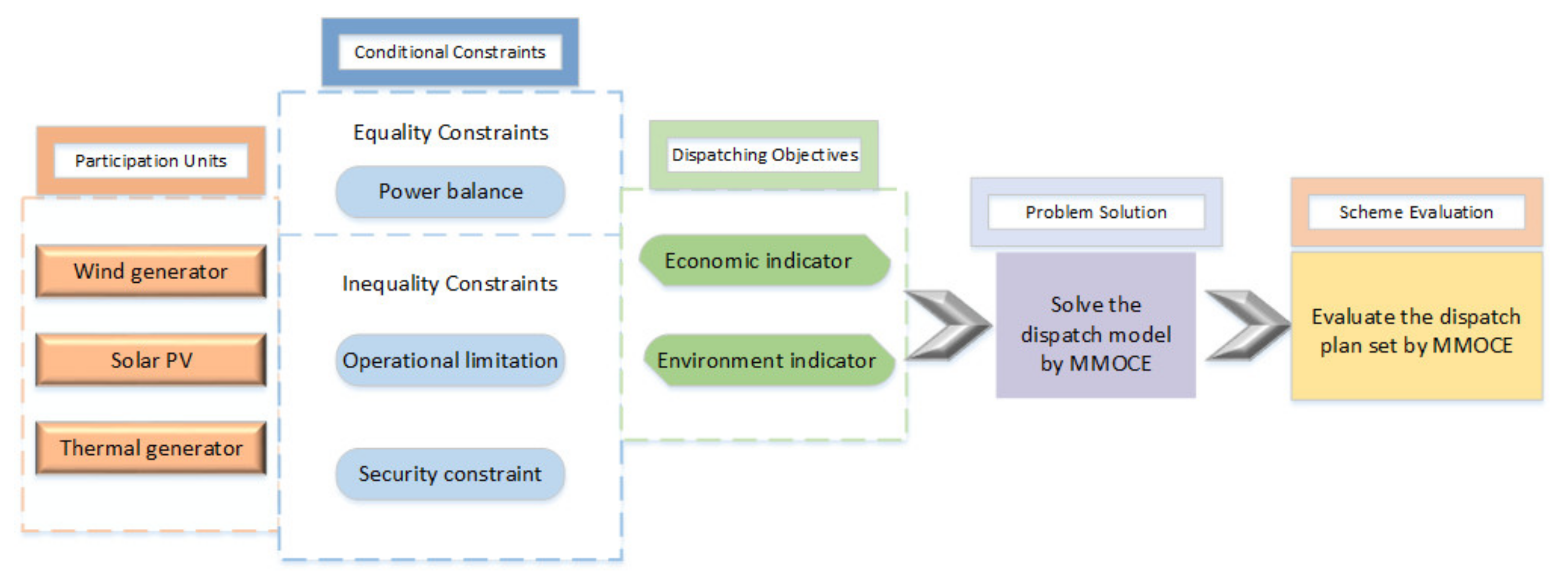
2. Mathematical Model
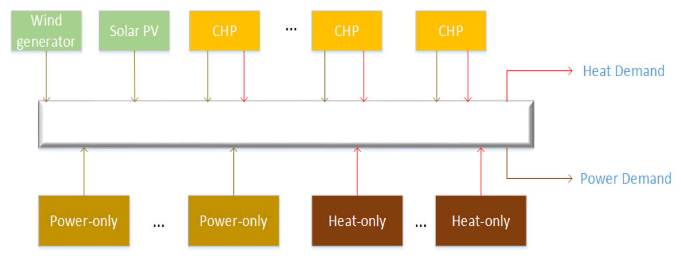
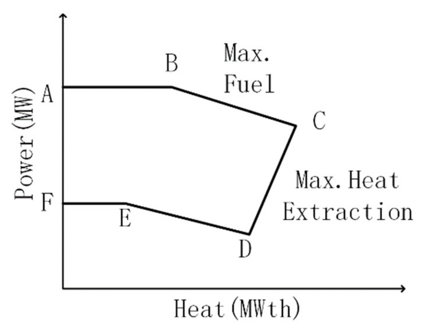
2.1. Problem Formulation of CHEED
2.1.1. Objective Functions
- Total cost is defined as:
- Emission is defined as:
2.1.2. Constraints
2.2. Mathematical Models of the Modified IEEE 30-Bus and Six-Generator System with Wind and Solar Energy
2.2.1. Cost of Conventional Thermal Units
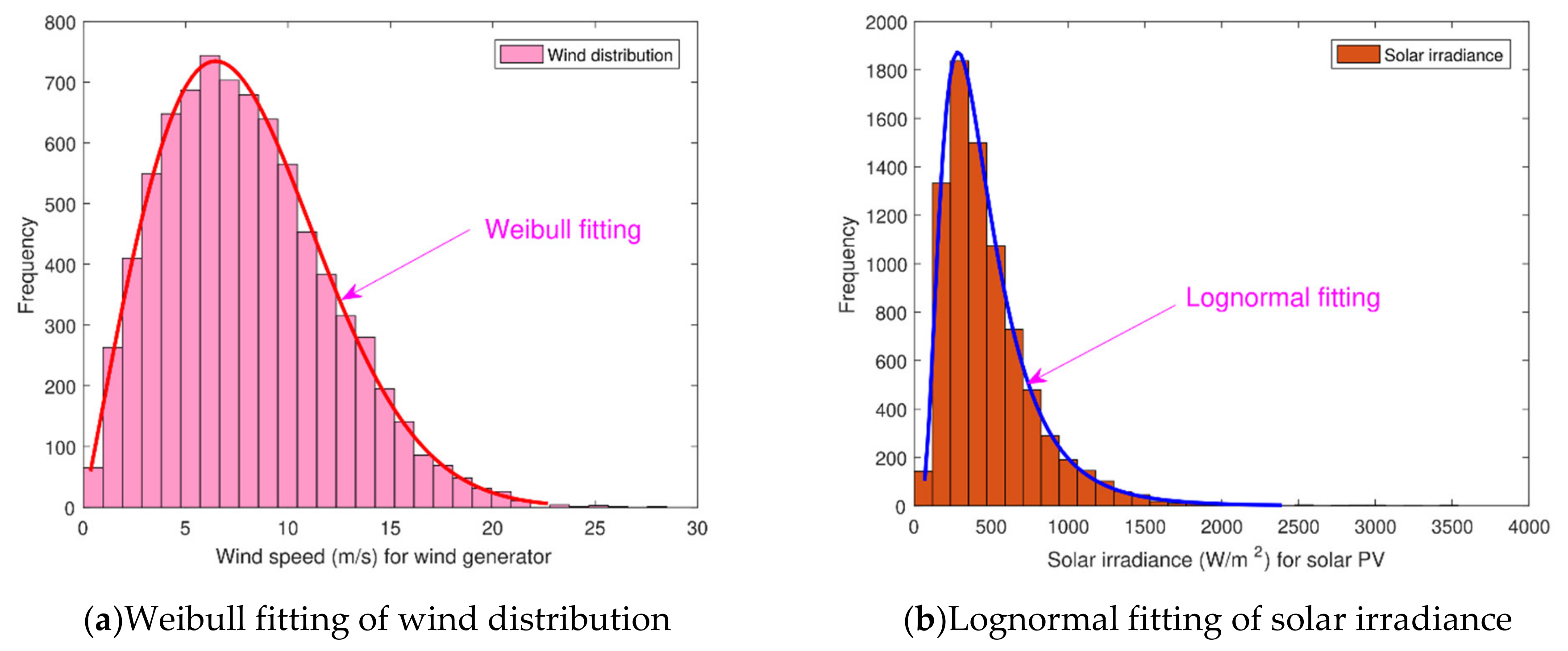
2.2.2. Cost of Wind Energy
2.2.3. Cost of Solar Photovoltaic Power
2.2.4. Emission Function
2.2.5. Objective Functions
2.2.6. Constraints
2.3. Combined Emission Economic Dispatch Problems with Wind Penetration
3. The Proposed Optimization Algorithm
3.1. Overview of the Cross Entropy Method
3.2. The Proposed Modified Multi-Objective Cross-Entropy Algorithm
3.2.1. Updating of Self-Adaptive Parameter
3.2.2. Crossover Operator
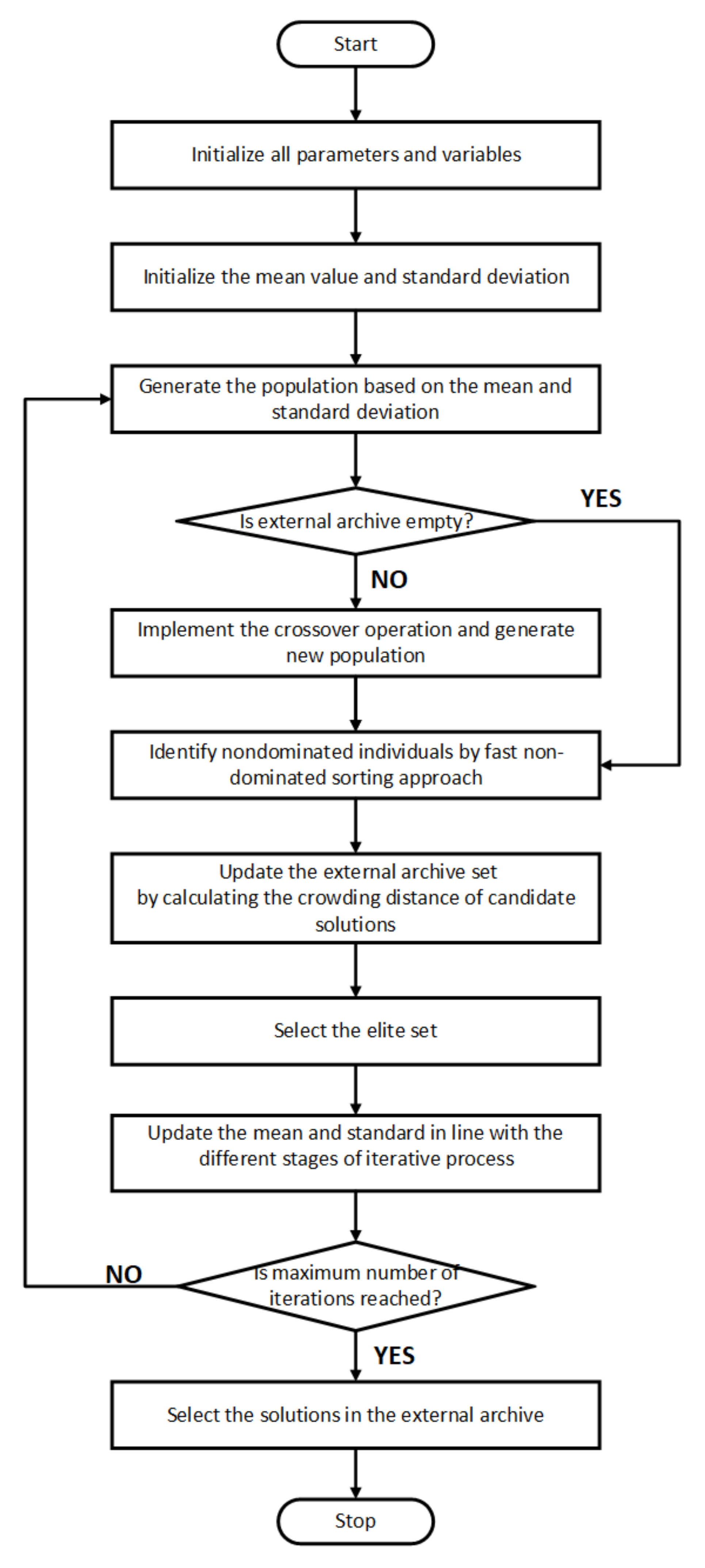
3.3. Implementation of MMOCE for EED
- Step 1. Input data. The feasible range of control variables, the population size , the maximum number of function evaluations Max_FES, the maximum size of external archive and the probability of crossover .
- Step 2. Initialization. The initial population is formed by normal distribution. It is assumed that the dimension n over ranges [, ], which denote the lower and upper limit, is assigned based on , where µ n is a random number between the lower and upper limit and σ n is set to 10 · (−), and FES = 0.
- Step 3. The mean value µ and standard deviation σ are updated by Equations (51)–(53). The endpoint value method is used as the boundary constraints handling strategy for the population .
- Step 4. The objective function values are calculated and coupled with a fast non-dominated sorting approach and crowding–distance metric to get the external archive.
- Step 5. The crossover operator is carried out by Equation (54).
- Step 6. The elite set is selected from the external archive and the different parameter evolutionary mechanisms are applied to update the mean value µ and standard deviation σ. FES = FES + .
- Step 7. Step 2 to Step 6 are repeated. If the termination criterion is met, i.e., Max_FES is reached, the above procedure is stopped.
4. Experimental Results
4.1. Experiments Based on Benchmark Functions
4.1.1. Inverted Generation Distance (IGD)
4.1.2. MaxSpread (MS)
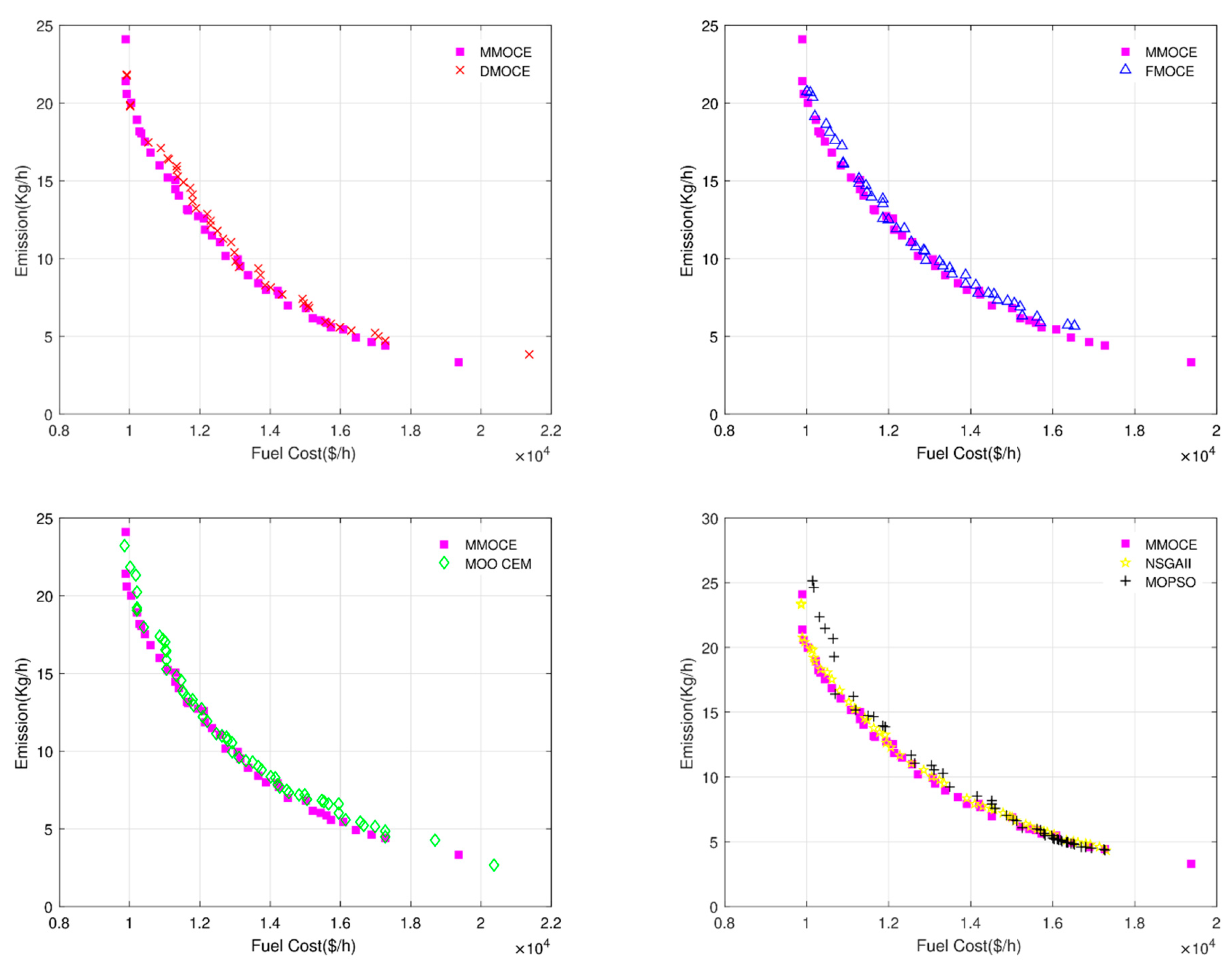
4.2. Simulation Results on Combined Heat, Emission, and Economic Dispatch (CHEED)
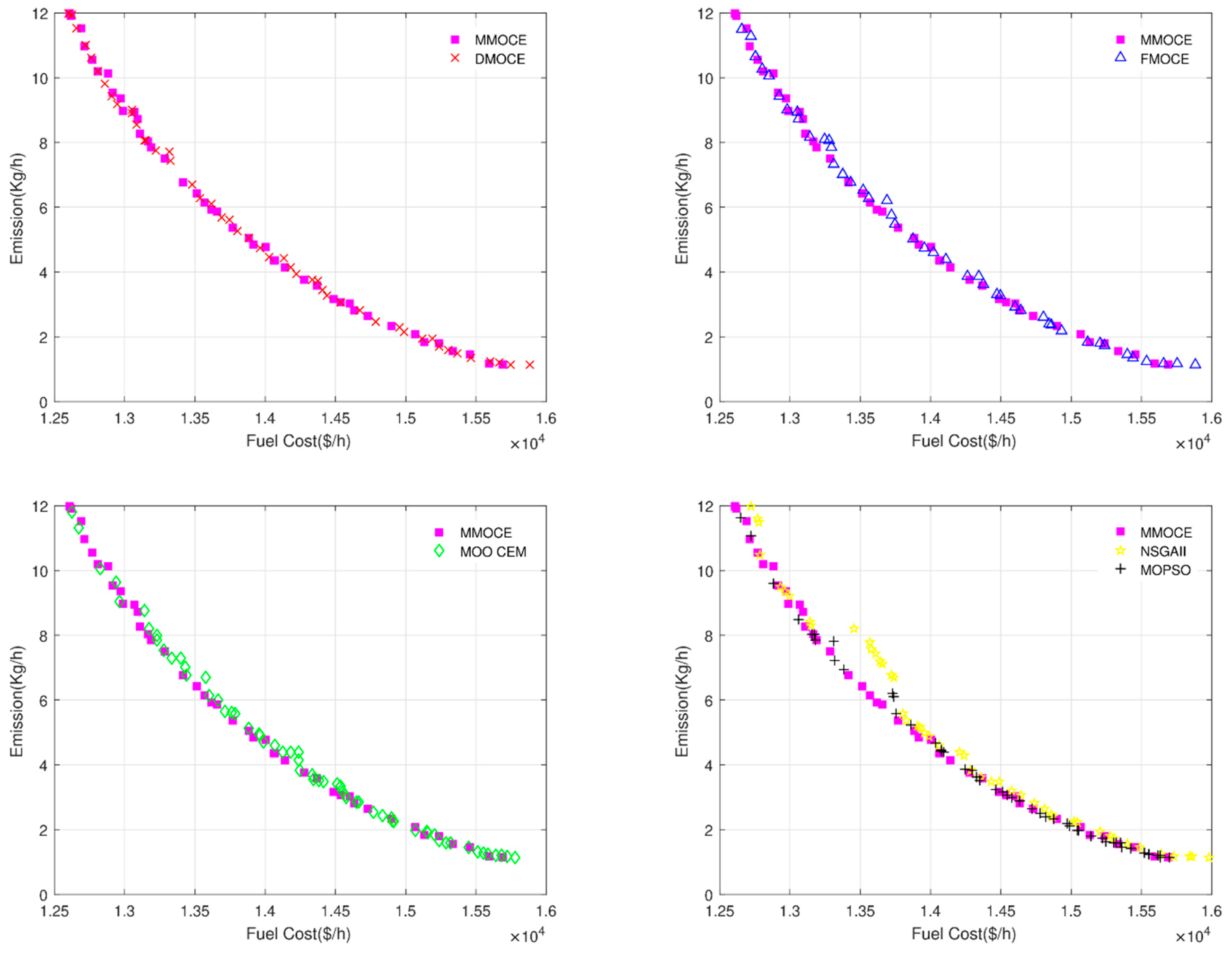
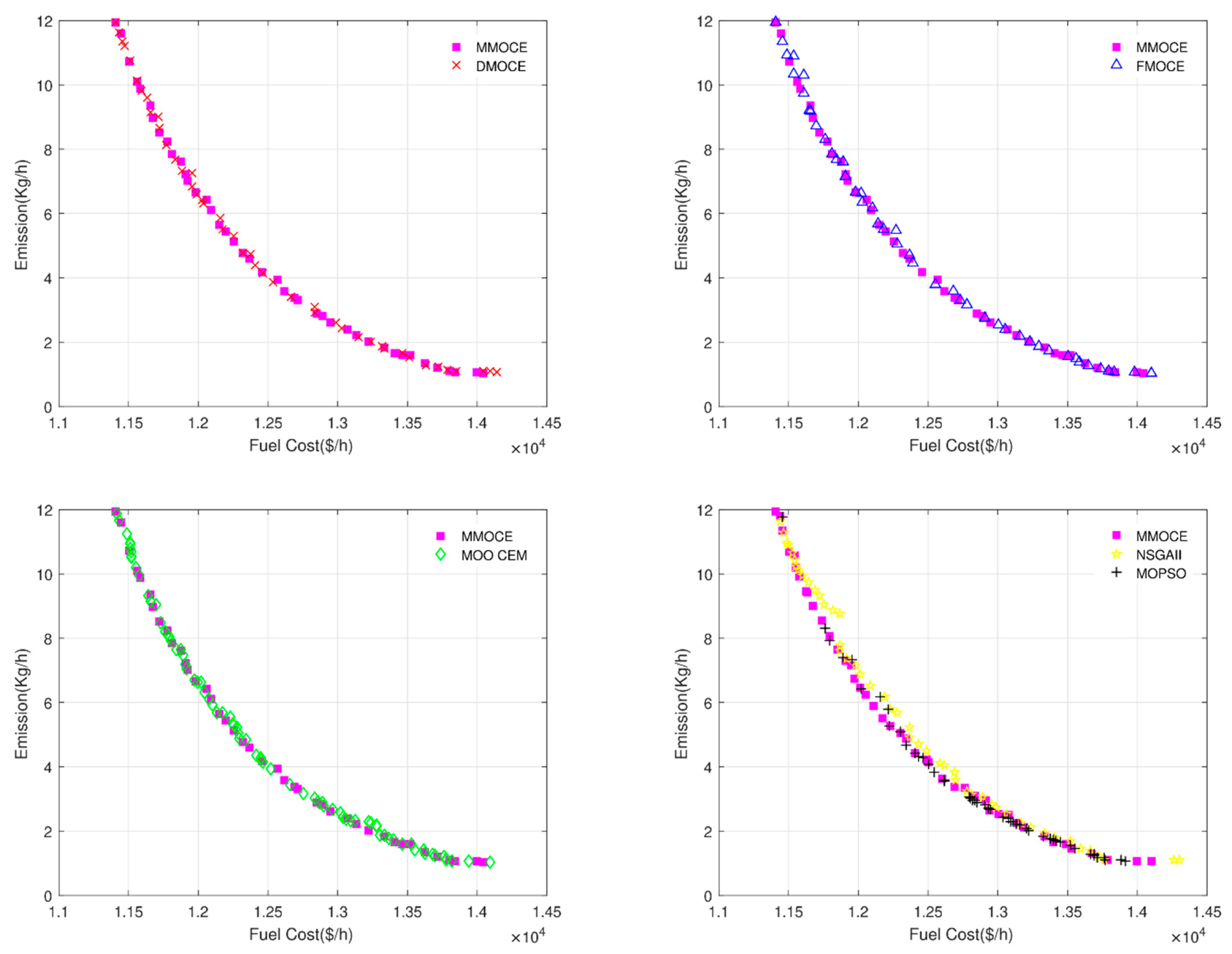
4.3. Simulation Results on IEEE 30-Bus with Six-Generator System
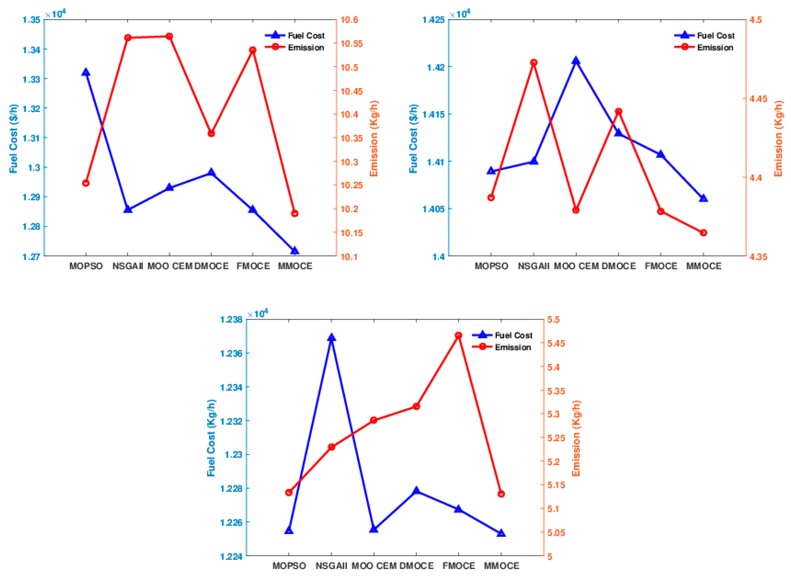
4.3.1. Case 1: System Incorporating Stochastic Wind and Solar
4.3.2. Case 2: The System Only Incorporating Stochastic Wind
4.3.3. Case 3: The System Only Incorporating Stochastic Solar PV
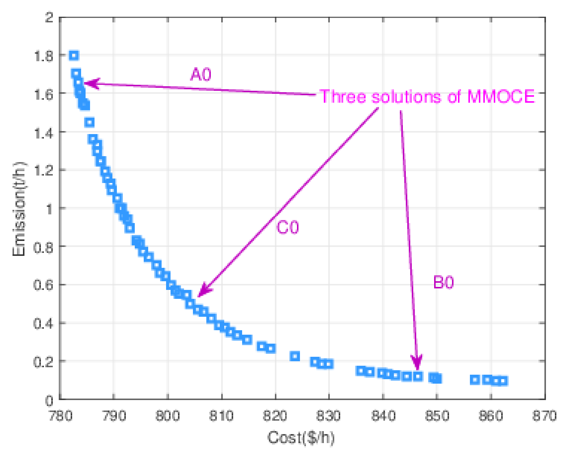
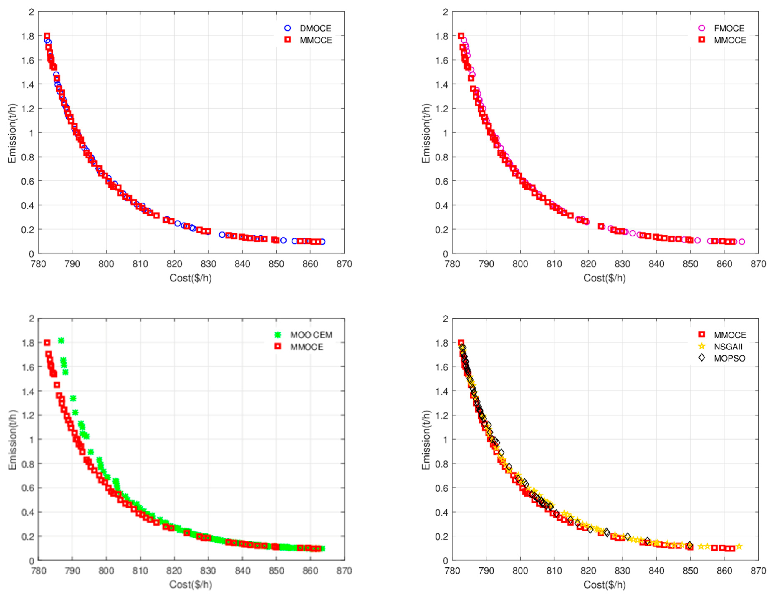
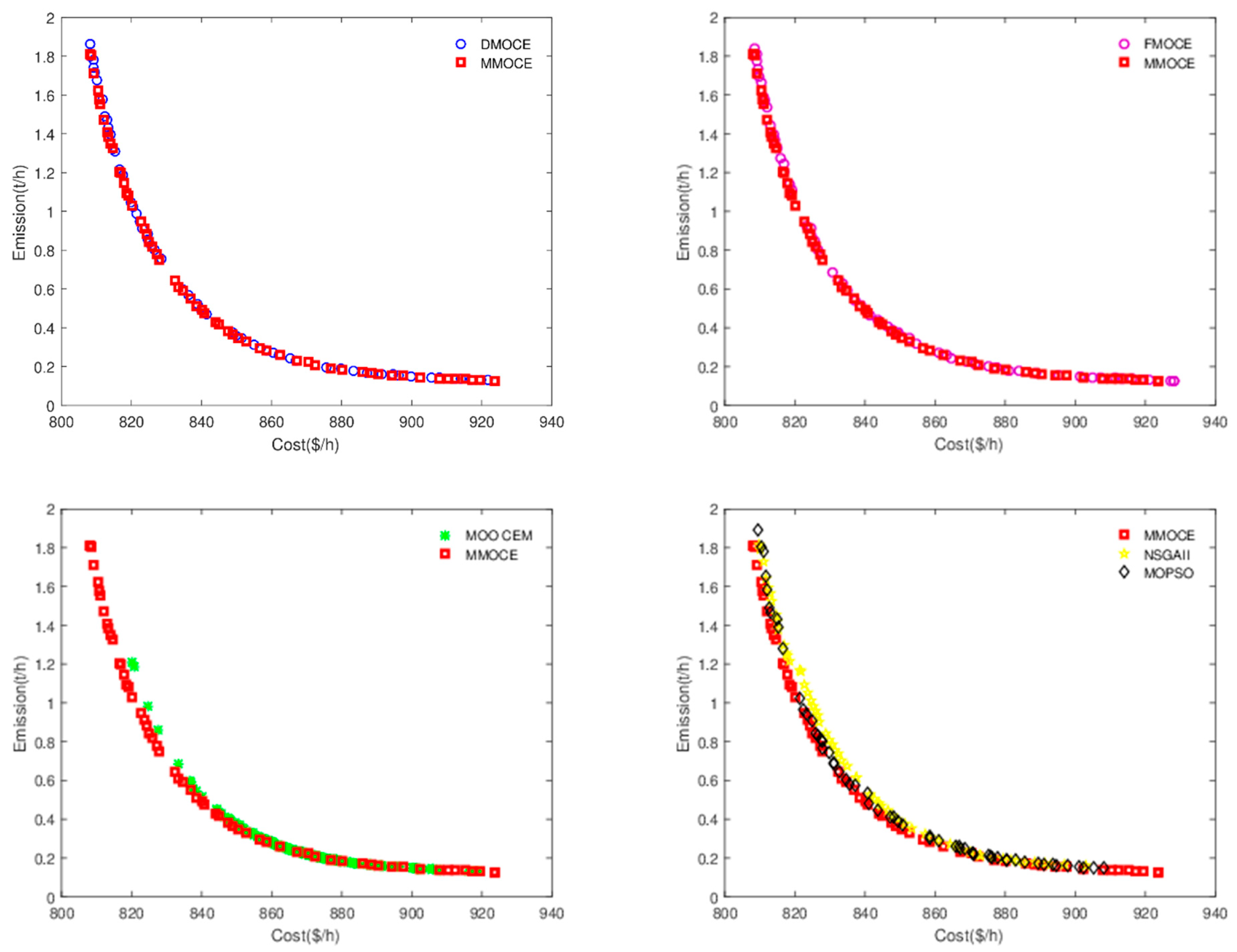
4.4. Combined Emission Economic Dispatch Problems with Wind Penetration
5. Conclusions
Author Contributions
Funding
Institutional Review Board Statement
Informed Consent Statement
Data Availability Statement
Acknowledgments
Conflicts of Interest
Nomenclature
| Total production cost | |
| Total emission | |
| Production cost of thermal power unit i | |
| Production cost of cogeneration unit j | |
| Production cost of heat-only unit k | |
| Emission of thermal power unit i | |
| Emission of cogeneration unit j | |
| Emission of heat-only unit k | |
| , | Load demand and transmission loss |
| , | Wind power and solar power |
| Total heat demand | |
| Power capacity limits of thermal power unit i | |
| Heat capacity limits of heat-only unit k | |
| Number of thermal power units | |
| Number of cogeneration units | |
| Number of heat-only units | |
| Cost coefficients for thermal power unit i | |
| Cost coefficients for cogeneration unit j | |
| Cost coefficients for heat-only unit k | |
| Emission coefficients for thermal power unit i | |
| Emission coefficients for cogeneration unit j | |
| Emission coefficients for heat-only unit k | |
| Total number of thermal power units | |
| Power produced by generating unit j | |
| Cost coefficients for thermal power unit j | |
| Valve effect coefficients for thermal power unit j | |
| Minimum power of thermal power unit j | |
| Cost constant of wind power unit i | |
| Scheduled wind power from unit i | |
| Reverse cost coefficient of wind unit i | |
| Actual available power of wind unit i | |
| Wind power probability function of wind unit i | |
| Penalty cost coefficient of wind unit i | |
| Rated output power of wind unit i | |
| Cut out wind speed, nominal wind speed, and cut in wind speed | |
| Rated power | |
| Current wind speed | |
| Cost constant of solar power unit j | |
| Scheduled solar power from unit j | |
| Reverse cost coefficient of solar power unit j | |
| Actual available power of solar power unit j | |
| Penalty cost coefficient of solar power unit j | |
| Emission coefficients for thermal power unit i |
References
- Chen, J.H.R.G.; Feng, E.N. Distributed Finite-Time Economic Dispatch of a Network of Energy Resources. IEEE Trans. Smart Grid 2016, 8, 1–11. [Google Scholar] [CrossRef]
- Chen, X.; Li, K.; Xu, B.; Yang, Z. Biogeography-based learning particle swarm optimization for combined heat and power economic dispatch problem. Knowl. Based Syst. 2020, 208, 106463. [Google Scholar] [CrossRef]
- Vo, D.H.; Vo, A.T.; Ho, C.M.; Nguyen, H.M. The Role of Renewable Energy, Alternative and Nuclear Energy in Mitigating Carbon Emissions in the CPTPP Countries. Renew. Energy 2020, 161, 278–292. [Google Scholar] [CrossRef]
- Tummala, A.; Velamati, R.K.; Sinha, D.K.; Indraja, V.; Krishna, V.H. A review on small scale wind turbines. Renew. Sustain. Energy Rev. 2016, 56, 1351–1371. [Google Scholar] [CrossRef]
- Aghaei, J.; Alizadeh, M.I. Demand Response in Smart Electricity Grids Equipped with Renewable Energy Sources: A Review. Renew. Sustain. Energy Rev. 2013, 18, 64–72. [Google Scholar] [CrossRef]
- Aramazd, M.; Steffi, O.M.; Galen, D.M.; Dakota, J.T.; Zachary, M.B.; Amro, M.F. The 2017 ISO New England System Operational Analysis and Renewable Energy Integration Study (SOARES). Energy Rep. 2019, 5, 747–792. [Google Scholar]
- Panwar, N.L.; Kaushik, S.C.; Kothari, S. Role of Renewable Energy Sources in Environmental Protection: A Review. Renew. Sustain. Energy Rev. 2011, 15, 1513–1524. [Google Scholar] [CrossRef]
- Mwasilu, F.; Justo, J.J.; Kim, E.K.; Do, T.D.; Jung, J.W. Electric Vehicles and Smart Grid Interaction: A Review on Vehicle to Grid and Renewable Energy Sources Integration. Renew. Sustain. Energy Rev. 2014, 34, 501–516. [Google Scholar] [CrossRef]
- Alomoush, M.I. Microgrid Combined Power-Heat Economic-Emission Dispatch Considering Stochastic Renewable Energy Resources, Power Purchase and Emission Tax. Energy Convers. Manag. 2019, 200, 112090. [Google Scholar] [CrossRef]
- Basu, M. Dynamic Economic Dispatch Incorporating Renewable Energy Sources and Pumped Hydroenergy Storage. Soft Comput. 2020, 24, 4829–4840. [Google Scholar] [CrossRef]
- Pluta, M.; Wyrwa, A.; Suwała, W.; Zyśk, J.; Raczyński, M.; Tokarski, S. A Generalized Unit Commitment and Economic Dispatch Approach for Analysing the Polish Power System under High Renewable Penetration. Energies 2020, 113, 1952. [Google Scholar] [CrossRef]
- Man-Im, A.; Ongsakul, W.; Madhu, N. Reliability Enhanced Multi-Objective Economic Dispatch Strategy for Hybrid Renewable Energy System with Storage. J. Oper. Res. Soc. China 2020, 1–31. [Google Scholar] [CrossRef]
- Omar, A.I.; Ali, Z.M.; Al-Gabalawy, M.; Abdel Aleem, S.H.; Al-Dhaifallah, M. Multi-Objective Environmental Economic Dispatch of an Electricity System Considering Integrated Natural Gas Units and Variable Renewable Energy Sources. Energies 2020, 8, 1100. [Google Scholar]
- Liu, T.; Jiao, L.; Ma, W.; Ma, J.; Shang, R. Cultural Quantum-Behaved Particle Swarm Optimization for Environmental/Economic Dispatch. Appl. Soft Comput. 2016, 48, 597–611. [Google Scholar] [CrossRef]
- Li, F.; Liang, H.; Liu, Y.; Shen, Y. A Multi-Objective Hybrid Bat Algorithm for Combined Economic/Emission Dispatch. Int. J. Electr. Power Energy Syst. 2018, 101, 103–115. [Google Scholar]
- Shilaja, C.; Ravi, K. Optimization of Emission/Economic Dispatch Using Euclidean Affine Flower Pollination Algorithm (eFPA) and Binary FPA (BFPA) in Solar Photo Voltaic Generation. Renew. Energy 2017, 107, 550–566. [Google Scholar] [CrossRef]
- Chen, J.; Gui, P.; Ding, T.; Na, S.; Zhou, Y. Optimization of Transportation Routing Problem for Fresh Food by Improved Ant Colony Algorithm Based on Tabu Search. Sustainability 2019, 11, 584. [Google Scholar] [CrossRef]
- Chen, J.J.; Qi, B.X.; Peng, K.; Li, Y.; Zhao, Y.L. Conditional Value-at-Credibility for Random Fuzzy Wind Power in Demand Response Integrated Multi-Period Economic Emission Dispatch. Appl. Energy 2020, 261, 114337. [Google Scholar] [CrossRef]
- Qiao, B.; Liu, J. Multi-Objective Dynamic Economic Emission Dispatch Based on Electric Vehicles and Wind Power Integrated System Using Differential Evolution Algorithm. Renew. Energy 2020, 154, 316–336. [Google Scholar] [CrossRef]
- Habibi, F.; Khosravi, F.; Kharrati, S.; Karimi, S. Simultaneous Multi-Area Economic-Environmental Load Dispatch Modeling in Presence of Wind Turbines by MOPSO. J. Electron. Eng. Technol. 2020, 15, 1059–1072. [Google Scholar] [CrossRef]
- Jiang, S.; Zhang, C.; Wu, W.; Chen, S. Combined Economic and Emission Dispatch Problem of Wind-Thermal Power System Using Gravitational Particle Swarm Optimization Algorithm. Math. Probl. Eng. 2019, 2019, 1–19. [Google Scholar] [CrossRef]
- Li, X.; Wang, W.; Wang, H.; Wu, J.; Fan, X.; Xu, Q. Dynamic Environmental Economic Dispatch of Hybrid Renewable Energy Systems Based on Tradable Green Certificates. Energy 2020, 193, 775–792. [Google Scholar] [CrossRef]
- Liao, H.L.; Wu, Q.H.; Li, Y.Z.; Jiang, L. Economic Emission Dispatching with Variations of Wind Power and Loads Using Multi-Objective Optimization by Learning Automata. Energy Convers. Manag. 2014, 87, 990–999. [Google Scholar] [CrossRef]
- Ghasemi, A.; Gheydi, M.; Golkar, M.J.; Eslami, M. Modeling of Wind/Environment/Economic Dispatch in Power System and Solving Via an Online Learning Meta-Heuristic Method. Appl. Soft Comput. 2016, 43, 454–468. [Google Scholar] [CrossRef]
- Rubinstein, R.Y. Optimization of Computer Simulation Models with Rare Events. Eur. J. Oper. Res. 1997, 99, 89–112. [Google Scholar] [CrossRef]
- Rubinstein, R. The Cross-Entropy Method for Combinatorial and Continuous Optimization. Methodol. Comput. Appl. Probab. 1999, 1, 127–190. [Google Scholar] [CrossRef]
- Gao, C.; Feng, Y.; Tong, X.; Jin, Y.; Gu, C. Modeling Urban Encroachment on Ecological Land Using Cellular Automata and Cross-Entropy Optimization Rules. Sci. Total Environ. 2020, 744, 140996. [Google Scholar] [CrossRef] [PubMed]
- Wang, L.; Li, Q.; Zhang, B.; Ding, R.; Sun, M. Robust Multi-Objective Optimization for Energy Production Scheduling in Microgrids. Eng. Optim. 2019, 51, 332–351. [Google Scholar] [CrossRef]
- Gu, X.; Yang, S.; Liu, Y. Multi-Objective Optimized Anti-Symmetric Real Laplace Wavelet Filter for Bearing Fault Diagnosis. In Proceedings of the International Conference on Sensing, Diagnostics, Prognostics, and Control, Shanghai, China, 16–18 August 2017; pp. 651–654. [Google Scholar]
- Selvakumar, A.I. Enhanced Cross-Entropy Method for Dynamic Economic Dispatch with Valve-Point Effects. Int. J. Electr. Power Energy Syst. 2011, 33, 783–790. [Google Scholar] [CrossRef]
- Ahmet, U.; Adnan, A. Multi-Objective Optimization with Cross Entropy Method: Stochastic Learning with Clustered Pareto Fronts. In Proceedings of the IEEE Congress on Evolutionary Computation, Singapore, 25–28 September 2007; pp. 3065–3071. [Google Scholar]
- Kar, M.B.; Majumder, S.; Kar, S.; Pal, T. Cross-Entropy Based Multi-Objective Uncertain Portfolio Selection Problem. J. Intell. Fuzzy Syst. Appl. Eng. Technol. 2017, 32, 4467–4483. [Google Scholar]
- Zhu, S.; Xu, W.; Fan, L.; Wang, K.; Karagiannidis, G.K. A Novel Cross Entropy Approach for Offloading Learning in Mobile Edge Computing. IEEE Wirel. Commun. Lett. 2020, 9, 402–405. [Google Scholar] [CrossRef]
- Beruvides, G.; Quiza, R.; Haber, R.E. Multi-Objective Optimization Based on an Improved Cross-Entropy Method. A Case Study of a Micro-Scale Manufacturing Process. Inf. Sci. 2016, 334, 161–173. [Google Scholar] [CrossRef]
- Zou, Y.; Xiao, J.; Huang, Z. A Multi-Objective Optimization Model for Coal Combustion in Thermal Power Plants. In Proceedings of the 2018 Chinese Automation Congress (CAC), Xi’an, China, 30 November–2 December 2018; pp. 655–660. [Google Scholar]
- Dorini, G.; Jonkergouw, P.; Kapelan, Z.; Di Pierro, F.; Khu, S.; Savic, D. An Efficient Algorithm for Sensor Placement in Water Distribution Systems. Water Distrib. Syst. Anal. Symp. 2008, 1–13. [Google Scholar]
- Xiang, L.; Sun, Y.; Ye, Z.; Jiang, C.; Lyu, J. Energy Route Multi-Objective Optimization of Wireless Power Transfer Network: An Improved Cross-Entropy Method. J. Electron. Syst. 2017, 13, 228–240. [Google Scholar]
- Perelman, L.; Ostfeld, A.; Salomons, E. Cross Entropy Multi-Objective Optimization for Water Distribution Systems Design. Water Resour. Res. 2008, 44, 542–547. [Google Scholar] [CrossRef]
- Bekker, J.; Aldrich, C. The Cross-Entropy Method in Multi-Objective Optimisation: An Assessment. Eur. J. Oper. Res. 2011, 211, 112–121. [Google Scholar] [CrossRef]
- Wang, G.; Zha, Y.; Wu, T.; Qiu, J.; Xu, G. Cross Entropy Optimization Based on Decomposition for Multi-Objective Economic Emission Dispatch Considering Renewable Energy Generation Uncertainties. Energy 2019, 193, 116790. [Google Scholar] [CrossRef]
- An, S.; Wang, W.; Yang, S. Vector Design Optimizations Using an Improved Cross-Entropy Method. IEEE Trans. Magn. 2015, 51, 1–4. [Google Scholar]
- Basu, M. Combined Heat and Power Economic Emission Dispatch Using Non-Dominated Sorting Genetic Algorithm-II. Int. J. Electron. Power Energy Syst. 2013, 53, 135–141. [Google Scholar] [CrossRef]
- Wood, A.J.; Wollenberg, B.F.; Sheblé, G.B. Power Generation Operation and Control; John Wiley & Sons: Hoboken, NJ, USA, 2013. [Google Scholar]
- Chen, C.L.; Lee, T.Y.; Jan, R.M. Optimal Wind-Thermal Coordination Dispatch in Isolated Power Systems with Large Integration of Wind Capacity. Energy Convers. Manag. 2006, 47, 3456–3472. [Google Scholar] [CrossRef]
- Biswas, P.P.; Suganthan, P.N.; Amaratunga, G.A.J. Optimal Power Flow Solutions Incorporating Stochastic Wind and Solar Power. Energy Convers. Manag. 2017, 148, 1194–1207. [Google Scholar] [CrossRef]
- Biswas, P.P.; Suganthan, P.N.; Qu, B.Y.; Amaratunga, G.A. Multi-Objective Economic-Environmental Power Dispatch with StoChastic Wind-Solar-Small Hydro Power. Energy 2018, 150, 1039–1057. [Google Scholar] [CrossRef]
- Panda, A.; Tripathy, M. Security Constrained Optimal Power Flow Solution of Wind-Thermal Generation System Using Modified Bacteria Foraging Algorithm. Energy 2015, 93, 816–827. [Google Scholar] [CrossRef]
- Dubey, H.M.; Pandit, M.; Panigrahi, B.K. Hybrid Flower Pollination Algorithm with Time-Varying Fuzzy Selection Mechanism for Wind Integrated Multi-Objective Dynamic Economic Dispatch. Renew. Energy 2015, 83, 188–202. [Google Scholar] [CrossRef]
- Chang, T.P. Investigation on Frequency Distribution of Global Radiation Using Different Probability Density Functions. Int. J. Appl. Eng. 2010, 8, 99–107. [Google Scholar]
- Deb, K.; Pratap, A.; Agarwal, S.; Meyarivan, T. A Fast and Elitist Multi-Objective Genetic Algorithm: NSGA-II. IEEE Trans. Evol. Comput. 2002, 6, 182–197. [Google Scholar] [CrossRef]
- Chen, X.; Du, W.; Qian, F. Multi-objective Differential Evolution with Ranking-Based Mutation Operator and Its Application in Chemical Process Optimization. Chemom. Intell. Lab. Syst. 2014, 136, 85–96. [Google Scholar] [CrossRef]
- Haber, R.E.; Beruvides, G.; Quiza, R.; Hernandez, A. A Simple Multi-Objective Optimization Based on the Cross-Entropy Method. IEEE Access 2017, 5, 22272–22281. [Google Scholar] [CrossRef]
- Tsai, S.J.; Sun, T.Y.; Liu, C.C.; Hsieh, S.T.; Wu, W.C.; Chiu, S.Y. An Improved Multi-objective Particle Swarm Optimizer for Multi-objective Problems. Exp. Syst. Appl. 2010, 37, 5872–5886. [Google Scholar] [CrossRef]
- Lu, Z.; Geng, L.; Huo, G.; Zhao, H.; Yao, W.; Li, G.; Guo, X.; Zhang, J. A Novel Hybrid Multi-objective Bacterial Colony Chemotaxis Algorithm. Soft Comput. 2019, 24, 2013–2032. [Google Scholar] [CrossRef]
- bin Mohd Zain, M.Z.; Kanesan, J.; Chuah, J.H.; Dhanapal, S.; Kendall, G. A Multi-Objective Particle Swarm Optimization Algorithm Based on Dynamic Boundary Search for Constrained Optimization. Appl. Soft Comput. 2018, 70, 680–700. [Google Scholar] [CrossRef]
- Elattar, E.E. Environmental Economic Dispatch with Heat Optimization in the Presence of Renewable Energy Based on Modified Shuffle Frog Leaping Algorithm. Energy 2019, 171, 256–269. [Google Scholar] [CrossRef]
- Devi, A.L.; Krishna, O.V. Combined Economic and Emission Dispatch Using Evolutionary Algorithms-A Case Study. ARPN J. Eng. Appl. Sci. 2008, 3, 28–35. [Google Scholar]
- Eusuff, M.; Lansey, K.; Pasha, F. Shuffled Frog-Leaping Algorithm: A Memetic Meta-Heuristic for Discrete Optimization: Engineering Optimization. Eng. Optim. 2006, 38, 129–154. [Google Scholar] [CrossRef]
- Basu, M. Teaching-Learning-Based Optimization Algorithm for Multi-Area Economic Dispatch. Energy 2014, 68, 21–28. [Google Scholar] [CrossRef]
- Li, X.; Luo, J.; Chen, M.R.; Wang, N. An Improved Shuffled Frog-Leaping Algorithm with Extremal Optimization for Continuous Optimization. Inf. Sci. 2012, 192, 143–151. [Google Scholar] [CrossRef]
- Chen, M.R.; Zeng, G.Q.; Lu, K.D. Constrained Multi-Objective Population Extremal Optimization Based Economic-Emission Dispatch Incorporating Renewable Energy Resources. Renew. Energy 2019, 143, 277–294. [Google Scholar] [CrossRef]
- Qu, B.Y.; Liang, J.J.; Zhu, Y.S.; Wang, Z.Y.; Suganthan, P.N. Economic Emission Dispatch Problems with Stochastic Wind Power Using Summation Based Multi-Objective Evolutionary Algorithm. Inf. Sci. 2016, 351, 48–66. [Google Scholar] [CrossRef]
- Barisal, A.K.; Prusty, R.C. Large Scale Economic Dispatch of Power Systems Using Oppositional Invasive Weed Optimization. Appl. Soft Comput. 2015, 29, 122–137. [Google Scholar] [CrossRef]
- Kheshti, M.; Ding, L.; Ma, S.; Zhao, B. Double Weighted Particle Swarm Optimization to Non-Convex Wind Penetrated Emission/Economic Dispatch and Multiple Fuel Option Systems. Renew. Energy 2018, 125, 1021–1037. [Google Scholar] [CrossRef]


| ZDT1 | ZDT2 | ZDT3 | UF1 | UF2 | UF3 | WFG1 | WFG2 | |
|---|---|---|---|---|---|---|---|---|
| 0.1 | 3.23 × 10⁻⁴ | 4.43 × 10⁻⁴ | 4.02E × 10−4 | 0.0051 | 0.0039 | 0.0226 | 0.0362 | 0.0257 |
| 0.2 | 2.64 × 10⁻⁴ | 2.62 × 10⁻⁴ | 2.89E × 10−4 | 0.0051 | 0.0030 | 0.0222 | 0.0352 | 0.0258 |
| 0.3 | 2.58 × 10⁻⁴ | 2.59 × 10⁻⁴ | 2.90E × 10−4 | 0.0052 | 0.0029 | 0.0225 | 0.0352 | 0.0257 |
| 0.382 | 2.57 × 10⁻⁴ | 2.58 × 10⁻⁴ | 2.85 × 10⁻⁴ | 0.0052 | 0.0029 | 0.0223 | 0.0351 | 0.0247 |
| 0.5 | 2.59 × 10⁻⁴ | 2.58 × 10⁻⁴ | 2.89 × 10⁻⁴ | 0.0052 | 0.0030 | 0.0234 | 0.0349 | 0.0271 |
| 0.6 | 2.65 × 10⁻⁴ | 2.65 × 10⁻⁴ | 2.99 × 10⁻⁴ | 0.0053 | 0.0032 | 0.0222 | 0.0348 | 0.0298 |
| 0.7 | 2.78 × 10⁻⁴ | 2.87 × 10⁻⁴ | 3.48 × 10⁻⁴ | 0.0055 | 0.0033 | 0.0224 | 0.0348 | 0.0284 |
| 0.8 | 2.97 × 10⁻⁴ | 0.0026 | 3.26 × 10⁻⁴ | 0.0055 | 0.0033 | 0.0248 | 0.0346 | 0.0287 |
| 0.9 | 2.94 × 10⁻⁴ | 0.0060 | 0.0010 | 0.0055 | 0.0035 | 0.0229 | 0.0347 | 0.0305 |
| 1.0 | 0.0013 | 0.0135 | 0.0017 | 0.0057 | 0.0040 | 0.0240 | 0.0346 | 0.0293 |
| ZDT1 | ZDT2 | ZDT3 | UF1 | UF2 | UF3 | WFG1 | WFG2 | |
|---|---|---|---|---|---|---|---|---|
| 0.1 | 1 | 1 | 0.9974 | 0.9955 | 0.9754 | 0.8170 | 0.6574 | 0.8072 |
| 0.2 | 1 | 1 | 0.9994 | 0.9987 | 0.9854 | 0.7510 | 0.6612 | 0.7899 |
| 0.3 | 1 | 1 | 0.9996 | 0.9991 | 0.9854 | 0.7518 | 0.6623 | 0.7814 |
| 0.382 | 1 | 1 | 0.9997 | 0.9994 | 0.9857 | 0.8602 | 0.6650 | 0.7800 |
| 0.5 | 0.9996 | 0.9998 | 0.9994 | 0.9991 | 0.9853 | 0.7160 | 0.6649 | 0.7493 |
| 0.6 | 0.9999 | 0.9990 | 0.9986 | 0.9985 | 0.9856 | 0.7351 | 0.6651 | 0.7463 |
| 0.7 | 0.9993 | 0.9979 | 0.9978 | 0.9958 | 0.9832 | 0.5762 | 0.6654 | 0.7227 |
| 0.8 | 0.9990 | 0.9438 | 0.9979 | 0.9930 | 0.9817 | 0.6401 | 0.6658 | 0.6888 |
| 0.9 | 0.9986 | 0.8798 | 0.9914 | 0.9957 | 0.9761 | 0.5692 | 0.6649 | 0.6783 |
| 1.0 | 0.9866 | 0.8222 | 0.9845 | 0.9934 | 0.9570 | 0.5633 | 0.6669 | 0.6730 |
| MODE | MOEA/D | MOPSO | NSGAII | PESAII | MMOCE | |
|---|---|---|---|---|---|---|
| ZDT1 | 0.0065 | 0.0072 | 0.0021 | 0.0263 | 0.0047 | 2.57 × 10⁻⁴ |
| ZDT2 | 0.0590 | 0.0569 | 0.0305 | 0.0524 | 0.0071 | 2.58 × 10⁻⁴ |
| ZDT3 | 0.0215 | 0.0157 | 0.0051 | 0.0322 | 0.0056 | 2.85 × 10⁻⁴ |
| UF1 | 0.0048 | 0.0178 | 0.0169 | 0.0178 | 0.0082 | 0.0052 |
| UF2 | 0.0024 | 0.0065 | 0.0099 | 0.0065 | 0.0059 | 0.0030 |
| UF3 | 0.0174 | 0.0225 | 0.0273 | 0.0271 | 0.0214 | 0.0223 |
| WFG1 | 0.0722 | 0.0352 | 0.0376 | 0.0440 | 0.0372 | 0.0351 |
| WFG2 | 0.0308 | 0.0540 | 0.0473 | 0.0529 | 0.0365 | 0.0247 |
| FMOCE | DMOCE | MOO CEM | SMOCE | MMOCE | |
|---|---|---|---|---|---|
| ZDT1 | 0.0031 | 3.4564E-04 | 0.0109 | 0.0192 | 2.5709 × 10⁻⁴ |
| ZDT2 | 0.0269 | 8.5574E-04 | 0.0015 | 0.0462 | 2.5821 × 10⁻⁴ |
| ZDT3 | 0.0046 | 4.6270E-04 | 0.0154 | 0.0162 | 2.8454 × 10⁻⁴ |
| UF1 | 0.0058 | 0.0053 | 0.0079 | 0.0077 | 0.0052 |
| UF2 | 0.0043 | 0.0030 | 0.0072 | 0.0046 | 0.0029 |
| UF3 | 0.0243 | 0.0211 | 0.0137 | 0.0186 | 0.0223 |
| WFG1 | 0.0358 | 0.0353 | 0.0937 | 0.0803 | 0.0351 |
| WFG2 | 0.0301 | 0.0289 | 0.0635 | 0.0452 | 0.0247 |
| MODE | MOEA/D | MOPSO | NSGAII | PESAII | MMOCE | |
|---|---|---|---|---|---|---|
| ZDT1 | 0.9091 | 0.8825 | 0.9830 | 0.7267 | 0.9066 | 0.9999 |
| ZDT2 | 0.7507 | 0.9269 | 0.9583 | 0.5724 | 0.8386 | 1.0000 |
| ZDT3 | 0.9264 | 0.7465 | 0.9414 | 0.6296 | 0.9429 | 0.9996 |
| UF1 | 0.8108 | 0.3753 | 0.8954 | 0.7695 | 0.7783 | 0.9994 |
| UF2 | 0.9398 | 0.6874 | 0.8911 | 0.9092 | 0.8606 | 0.9837 |
| UF3 | 0.5529 | 0.1912 | 0.4928 | 0.5289 | 0.4153 | 0.8602 |
| WFG1 | 0.1796 | 0.5308 | 0.5819 | 0.3302 | 0.6397 | 0.6650 |
| WFG2 | 0.6554 | 0.4462 | 0.5437 | 0.4455 | 0.6282 | 0.7800 |
| FMOCE | DMOCE | MOO CEM | SMOCE | MMOCE | |
|---|---|---|---|---|---|
| ZDT1 | 0.9947 | 0.9989 | 0.9712 | 0.7461 | 0.9999 |
| ZDT2 | 0.8573 | 0.9811 | 0.9693 | 0.7446 | 1.0000 |
| ZDT3 | 0.9680 | 0.9972 | 0.9350 | 0.8211 | 0.9996 |
| UF1 | 0.9909 | 0.9990 | 0.7454 | 0.8489 | 0.9994 |
| UF2 | 0.9464 | 0.9724 | 0.9349 | 0.8679 | 0.9837 |
| UF3 | 0.4954 | 0.5511 | 0.7204 | 0.5759 | 0.8602 |
| WFG1 | 0.6631 | 0.6621 | 0.2891 | 0.2589 | 0.6650 |
| WFG2 | 0.7146 | 0.6942 | 0.4726 | 0.5242 | 0.7800 |
| MODE | MOEA/D | MOPSO | NSGAII | PESAII | MMOCE | |
|---|---|---|---|---|---|---|
| ZDT1 | 32.94 | 124.91 | 25.95 | 2.85 | 52.72 | 2.69 |
| ZDT2 | 31.67 | 124.56 | 4.16 | 5.71 | 42.26 | 3.08 |
| ZDT3 | 31.75 | 127.96 | 8.19 | 3.78 | 44.60 | 5.28 |
| UF1 | 31.67 | 128.73 | 6.70 | 6.02 | 29.42 | 10.38 |
| UF2 | 44.40 | 130.96 | 9.69 | 3.69 | 55.84 | 5.93 |
| UF3 | 40.87 | 139.01 | 18.26 | 3.79 | 50.44 | 11.19 |
| WFG1 | 55.59 | 131.20 | 20.48 | 4.46 | 70.60 | 3.21 |
| WFG2 | 52.88 | 126.48 | 6.66 | 4.53 | 41.68 | 8.19 |
| Method | ||||||
|---|---|---|---|---|---|---|
| GA [57] | SFLA [58] | TLBO [59] | ISFLA [60] | MSFLA [56] | MMOCE | |
| 38.8755 | 48.3207 | 40.0649 | 39.3109 | 40.3650 | 35.6071 | |
| 53.7749 | 38.3751 | 51.0577 | 51.0506 | 51.0577 | 31.4136 | |
| 63.1298 | 61.5122 | 51.7601 | 51.9601 | 50.6388 | 47.6949 | |
| 58.3387 | 65.9934 | 72.4301 | 72.9411 | 72.0309 | 77.4051 | |
| 219.8752 | 219.8752 | 217.2403 | 217.4305 | 219.8752 | 245.8501 | |
| 75.9912 | 75.9912 | 74.9801 | 74.9731 | 75.9912 | 0.0000 | |
| 112.5602 | 112.5602 | 113.9616 | 113.8016 | 112.5602 | 108.4909 | |
| 69.4130 | 69.4130 | 69.1130 | 69.1030 | 69.4130 | 71.1467 | |
| 4.5957 | 4.5957 | 5.9071 | 5.9244 | 4.5957 | 78.8533 | |
| 6.5532 | 6.5440 | 6.5104 | 6.4942 | 6.4926 | 6.4818 | |
| Fuel Cost | 16,345.2433 | 16,351.3678 | 16,314.2368 | 16,312.2403 | 16,344.6539 | 16,286.4264 |
| Emission | 6.0373 | 6.0021 | 5.9616 | 5.9572 | 5.9054 | 5.0793 |
| Total Cost | 157,660.9862 | 156,844.7707 | 155,859.8997 | 155,752.9672 | 154,574.6139 | 135,178.7443 |
| Method | ||||||
|---|---|---|---|---|---|---|
| GA [57] | SFLA [58] | TLBO [59] | ISFLA [60] | MSFLA [56] | MMOCE | |
| 36.2567 | 35.0000 | 35.1000 | 35.0400 | 35.0000 | 35.0327 | |
| 120.7361 | 105.7361 | 104.1568 | 104.3659 | 105.7361 | 107.2488 | |
| 65.5581 | 80.0100 | 91.7052 | 91.8122 | 92.0100 | 99.4770 | |
| 24.6440 | 47.7440 | 44.2212 | 44.0821 | 42.7440 | 22.7183 | |
| 44.0943 | 42.0943 | 42.3921 | 42.3844 | 42.0943 | 50.5230 | |
| 88.3632 | 81.5200 | 86.5220 | 86.5120 | 86.5200 | 105.0000 | |
| 40.3476 | 27.9037 | 15.9027 | 15.8034 | 15.9037 | 0.0000 | |
| 0.0000 | 0.0000 | 0.0000 | 0.0000 | 0.0000 | 0.0000 | |
| Fuel Cost | 15,891.4751 | 15,955.0000 | 15,883.9895 | 15,886.4598 | 15,889.0000 | 15,716.8701 |
| Emission | 1.1840 | 1.1452 | 1.1448 | 1.1421 | 1.1397 | 1.1199 |
| Total Cost | 58,355.0346 | 57,025.0000 | 56,940.3826 | 56,847.1008 | 56,761.0001 | 55,879.9631 |
| Method | ||||||
|---|---|---|---|---|---|---|
| GA [57] | SFLA [58] | TLBO [59] | ISFLA [60] | MSFLA [56] | MMOCE | |
| 35.0356 | 35.0356 | 35.1688 | 35.2656 | 35.0356 | 35.0000 | |
| 95.0011 | 112.0611 | 112.5303 | 112.5013 | 112.0611 | 87.4635 | |
| 101.8674 | 107.8674 | 107.5905 | 107.8003 | 107.8674 | 112.6999 | |
| 38.4637 | 17.8637 | 10.4471 | 10.3338 | 10.4640 | 10.7293 | |
| 42.8607 | 38.8607 | 38.8596 | 38.8596 | 38.8607 | 40.3126 | |
| 56.5000 | 59.5000 | 66.8542 | 66.8993 | 66.8993 | 91.8075 | |
| 28.2738 | 28.2738 | 28.5500 | 28.3401 | 28.2738 | 21.9875 | |
| 2.0000 | 0.0002 | 0.0000 | 0.0000 | 0.0002 | 0.0000 | |
| Fuel Cost | 14,421.0000 | 14,464.6435 | 14,389.7481 | 14,392.9789 | 14,397.6852 | 14,064.4171 |
| Emission | 1.0845 | 1.0681 | 1.0699 | 1.0658 | 1.0600 | 1.0449 |
| Total Cost | 45,110.0000 | 44,691.5777 | 44,665.9095 | 44,552.4498 | 44,393.2696 | 43,632.8405 |
| Algorithms | Fuel Cost ($/h) | Emission (Kg/h) |
|---|---|---|
| MMOCE | 12,714.9326 | 10.1900 |
| FMOCE | 12,854.2320 | 10.5354 |
| DMOCE | 12,979.9436 | 10.3582 |
| MOO CEM | 12,929.2931 | 10.5643 |
| NSGAII | 12,855.0487 | 10.5610 |
| MOPSO | 13,319.9367 | 10.2544 |
| Algorithms | Fuel Cost ($/h) | Emission (Kg/h) |
|---|---|---|
| MMOCE | 14,059.9237 | 4.3645 |
| FMOCE | 14,106.7250 | 4.3783 |
| DMOCE | 14,129.1889 | 4.4418 |
| MOO CEM | 14,205.7126 | 4.3789 |
| NSGAII | 14,099.5992 | 4.4725 |
| MOPSO | 14,089.1572 | 4.3871 |
| Algorithms | Fuel Cost ($/h) | Emission (Kg/h) |
|---|---|---|
| MMOCE | 12,252.9253 | 5.1305 |
| FMOCE | 12,267.3198 | 5.4654 |
| DMOCE | 12,278.0982 | 5.3153 |
| MOO CEM | 12,255.3025 | 5.2858 |
| NSGAII | 12,368.6973 | 5.2289 |
| MOPSO | 12,254.4826 | 5.1332 |
| Control Variables | Min | Max | MMOCE | SHADE [45] | ||
|---|---|---|---|---|---|---|
| (MW) | 50 | 140 | 122.352 | 128.012 | 120.35 | 123.525 |
| (MW) | 20 | 80 | 32.955 | 31.274 | 32.955 | 33.047 |
| (MW) | 10 | 35 | 10 | 10 | 10.124 | 10 |
| (MW) | 0 | 75 | 45.898 | 43.969 | 45.898 | 37.336 |
| (MW) | 0 | 60 | 38.43 | 37.663 | 40.203 | 46.021 |
| (MW) | 0 | 50 | 38.998 | 38.022 | 38.998 | 38.748 |
| (p.u.) | 0.95 | 1.10 | 1.067 | 1.067 | 1.067 | 1.071 |
| (p.u.) | 0.95 | 1.10 | 1.052 | 1.053 | 1.053 | 1.057 |
| (p.u.) | 0.95 | 1.10 | 1.035 | 1.032 | 1.035 | 1.036 |
| (p.u.) | 0.95 | 1.10 | 1.10 | 1.1 | 1.1 | 1.04 |
| (p.u.) | 0.95 | 1.10 | 1.10 | 1.1 | 1.1 | 1.099 |
| (p.u.) | 0.95 | 1.10 | 1.067 | 1.061 | 1.067 | 1.056 |
| (MW) | −20 | 150 | −0.492 | −4.186 | −7.608 | 2.678 |
| (MW) | −20 | 60 | 0.2381 | 9.35 | 8.031 | 12.319 |
| (MW) | −15 | 40 | 40 | 40 | 40 | 35.27 |
| (MW) | −30 | 35 | 24.184 | 21.62 | 23.429 | 22.964 |
| (MW) | −25 | 30 | 30 | 30 | 30 | 30 |
| (MW) | −20 | 25 | 21.871 | 19.797 | 21.859 | 17.779 |
| ($/h) | 17.83 | 17.83 | 17.83 | 17.83 | ||
| Cost ($/h) | 794.231 | 788.802 | 796.386 | / | ||
| Emission (t/h) | 0.833 | 1.16 | 0.744 | 0.891 | ||
| Tatal Cost ($/h) | 809.060 | 809.478 | 809.655 | 810.346 | ||
| Control Variables | Cost-Solution (A0, A1, A2) | Emission-Solution (B0, B1, B2) | Compromise-Solution (C0, C1, C2) | ||||||
|---|---|---|---|---|---|---|---|---|---|
| MMOCE | CMOEO-EED [61] | CNSGAII-EED [62] | MMOCE | CMOEO-EED [61] | CNSGAII-EED [62] | MMOCE | CMOEO-EED [61] | CNSGAII-EED [62] | |
| (MW) | 133.9071 | 134.2443 | 135.0588 | 69.1754 | 67.8734 | 72.1327 | 112.9751 | 113.6415 | 116.5484 |
| (MW) | 26.9556 | 22.7365 | 24.0749 | 55.7616 | 52.4909 | 41.8570 | 37.0689 | 39.3716 | 36.2704 |
| (MW) | 10 | 10.3261 | 16.8847 | 19.1664 | 14.3867 | 21.0405 | 10 | 10 | 16.6980 |
| (MW) | 43.9685 | 44.4640 | 44.5520 | 54. 2363 | 54.7671 | 63.3223 | 49.9448 | 45.5167 | 45.0197 |
| (MW) | 36.0219 | 39.3188 | 31.4980 | 46.6161 | 49.2786 | 46.7542 | 39.5683 | 38.7017 | 37.4236 |
| (MW) | 38.2984 | 37.4988 | 37.4310 | 41.9088 | 48.0108 | 41.8268 | 38.6851 | 41.2587 | 36.9400 |
| (p.u.) | 1.0699 | 1.0749 | 1.0783 | 1.0665 | 1.0581 | 1.0783 | 1.0637 | 1.0581 | 1.0784 |
| (p.u.) | 1.0522 | 1.0606 | 0.9976 | 1.0413 | 1.0470 | 0.9917 | 1.0527 | 1.0516 | 0.9971 |
| (p.u.) | 1.0335 | 1.1000 | 1.0933 | 1.0323 | 1.1000 | 1.0933 | 1.0390 | 1.1000 | 1.0933 |
| (p.u.) | 1.1000 | 1.0453 | 1.1000 | 1.1000 | 1.0412 | 1.1000 | 1.0988 | 1.0341 | 1.0999 |
| (p.u.) | 1.0994 | 1.1000 | 1.0012 | 1.0994 | 1.1000 | 0.9868 | 1.0999 | 1.1000 | 0.9869 |
| (p.u.) | 1.0644 | 1.0084 | 1.1000 | 1.0567 | 1.1000 | 1.1000 | 1.0621 | 1.0637 | 1.0964 |
| (MW) | 2.1452 | −1.2440 | 35.9874 | 20.7012 | 1.5847 | 35.2648 | −7.8702 | −17.8574 | 38.7056 |
| (MW) | 0.3507 | 16.2791 | −20 | −20 | −14.1580 | −20 | 5.6642 | 16.9428 | −20 |
| (MW) | 40 | 40 | 40 | 40 | 40 | 40 | 40 | 40 | 40 |
| (MW) | 23.7233 | 31.1651 | 35 | 21.7630 | 29.7936 | 35 | 26.6124 | 24.9220 | 35 |
| (MW) | 29.8159 | 30 | 1.2666 | 30 | 30 | −3.6728 | 30 | 30 | −2.2033 |
| (MW) | 20.9158 | 1.4444 | 25 | 19.0388 | 25 | 25 | 20.0658 | 21.5430 | 25 |
| Cost ($/h) | 783.3389 | 784.0305 | 789.4062 | 846.5224 | 846.5317 | 848.2084 | 804.2061 | 804.5355 | 805.5781 |
| Emission | 1.6573 | 1.6931 | 1.7783 | 0.1168 | 0.1152 | 0.1215 | 0.4994 | 0.5167 | 0.6018 |
| MMOCE | DMOCE | FMOCE | MOO CEM | NSGAII | MOPSO | |
|---|---|---|---|---|---|---|
| (MW) | 112.9751 | 113.0508 | 113.2180 | 113.9853 | 114.3649 | 113.5886 |
| (MW) | 37.0689 | 38.9045 | 34.0862 | 30.6144 | 41.1093 | 40.9433 |
| (MW) | 10 | 10 | 10 | 10.4010 | 11.1905 | 10.0105 |
| (MW) | 49.9448 | 47.3610 | 50.4035 | 51.6109 | 42.2642 | 49.0710 |
| (MW) | 39.5689 | 39.3637 | 41.8038 | 41.5601 | 43.9396 | 36.1924 |
| (MW) | 36.6851 | 39.6871 | 38.7534 | 40.3542 | 35.7173 | 38.7900 |
| (p.u.) | 1.0637 | 1.0647 | 1.0735 | 1.0553 | 1.0646 | 1.0776 |
| (p.u.) | 1.0527 | 1.0509 | 0.9567 | 0.9702 | 0.9807 | 1.0267 |
| (p.u.) | 1.0390 | 1.0294 | 1.0350 | 1.0365 | 1.0856 | 1.0830 |
| (p.u.) | 1.0988 | 1.0361 | 1.0988 | 1.0323 | 1.0858 | 1.0952 |
| (p.u.) | 1.0999 | 1.1000 | 1.0848 | 1.0329 | 1.0999 | 1.0664 |
| (p.u.) | 1.0621 | 1.0490 | 1.0585 | 1.0243 | 1.0862 | 1.0198 |
| (MW) | −7.8702 | 0.2431 | 22.7539 | 27.1743 | 6.5293 | 29.8476 |
| (MW) | 5.6642 | 8.4721 | −20 | −20 | −20 | −20 |
| (MW) | 40 | 37.6685 | 40 | 40 | 40 | 40 |
| (MW) | 26.6124 | 21.6926 | 25.7524 | 35 | 35 | 35 |
| (MW) | 30 | 30 | 26.0320 | 17.1734 | 30 | 22.964 |
| (MW) | 20.0658 | 17.2351 | 20.1288 | 17.6723 | 25 | 8.0319 |
| Cost ($/h) | 804.2061 | 804.3160 | 804.4383 | 805.7037 | 806.0331 | 804.8684 |
| Emission (t/h) | 0.4994 | 0.5011 | 0.5016 | 0.5273 | 0.5362 | 0.5151 |
| Control Variables | Cost-Solution (A0, A1, A2) | Emission-Solution (B0, B1, B2) | Compromise-Solution (C0, C1, C2) | ||||||
|---|---|---|---|---|---|---|---|---|---|
| MMOCE | CMOEO-EED [61] | CNSGAII-EED [62] | MMOCE | CMOEO-EED [61] | CNSGAII-EED [62] | MMOCE | CMOEO-EED [61] | CNSGAII-EED [62] | |
| (MW) | 133.0246 | 133.4204 | 136.1377 | 70.7194 | 66.0442 | 71.0043 | 114.3254 | 114.3152 | 117.6553 |
| (MW) | 41.6542 | 36.4690 | 32.7275 | 58.6058 | 60.0168 | 57.9792 | 55.9144 | 49.4717 | 48.4645 |
| (MW) | 10 | 11.0759 | 20.4909 | 24.2350 | 35 | 31.2133 | 10.3215 | 11.3607 | 22.6222 |
| (MW) | 12 | 12 | 13.1202 | 23.6914 | 12 | 21.8278 | 12 | 12 | 13.1951 |
| (MW) | 49.5673 | 52.6521 | 50.1389 | 60.8875 | 62.1738 | 57.9794 | 52.9072 | 57.7254 | 50.1389 |
| (MW) | 42.9147 | 43.4150 | 36.7650 | 48.4544 | 51.1847 | 46.9542 | 43.0633 | 43.4150 | 36.7531 |
| (p.u.) | 1.0720 | 1.0638 | 1.0903 | 1.0652 | 1.0626 | 1.0817 | 1.0694 | 1.0667 | 1.0903 |
| (p.u.) | 1.0591 | 1.0530 | 0.9701 | 1.0587 | 1.0530 | 0.9705 | 1.0558 | 1.0584 | 0.9712 |
| (p.u.) | 1.0388 | 1.1000 | 1.0944 | 1.0396 | 1.1000 | 1.1000 | 1.0379 | 1.1000 | 1.0837 |
| (p.u.) | 1.0553 | 1.0650 | 0.9875 | 1.0565 | 1.0497 | 0.9905 | 1.0574 | 1.0585 | 0.9855 |
| (p.u.) | 1.0800 | 1.0359 | 1.0726 | 1.0926 | 1.0424 | 1.0737 | 1.1000 | 1.0441 | 1.0727 |
| (p.u.) | 1.0511 | 1.1000 | 1.0555 | 1.0510 | 1.1000 | 1.0574 | 1.0510 | 1.1000 | 1.0567 |
| (MW) | −4.0466 | −11.6123 | 45.3146 | −4.2832 | 2.9649 | 38.4253 | 1.3983 | −11.3175 | 44.8153 |
| (MW) | 15.6637 | 13.3567 | −20 | 11.4685 | −3.9619 | −20 | 3.8894 | 12.5536 | −20 |
| (MW) | 40 | 40 | 40 | 40 | 40 | 40 | 40 | 40 | 40 |
| (MW) | 18.2106 | 23.0313 | −1.6361 | 16.0053 | 16.6208 | −1.9824 | 17.5542 | 19.1638 | −2.8490 |
| (MW) | 24.1201 | 23.7141 | 35 | 18.9026 | 25.1861 | 35 | 23.8134 | 25.3184 | 35 |
| (MW) | 24.2296 | 30 | 20.0770 | 27.9365 | 30 | 20.2949 | 30 | 29.8266 | 20.0146 |
| Cost ($/h) | 810.3276 | 810.6380 | 814.6888 | 888.5777 | 888.5999 | 888.9853 | 834.5583 | 834.6694 | 835.5906 |
| Emission | 1.6216 | 1.6618 | 1.9532 | 0.1645 | 0.1664 | 0.1706 | 0.5896 | 0.5899 | 0.6924 |
| MMOCE | DMOCE | FMOCE | MOO CEM | NSGAII | MOPSO | |
|---|---|---|---|---|---|---|
| (MW) | 114.3254 | 114.6435 | 114.4487 | 114.6034 | 117.1215 | 114.9084 |
| (MW) | 55.9144 | 57.6041 | 50.0948 | 50.9100 | 42.1368 | 53.3999 |
| (MW) | 10.3215 | 10 | 13.4001 | 15.1987 | 17.4805 | 10.0105 |
| (MW) | 12 | 12 | 12 | 12 | 16.3096 | 12.7678 |
| (MW) | 52.9072 | 51.6911 | 55.0908 | 50.1419 | 51.6231 | 52.8663 |
| (MW) | 43.0633 | 42.7644 | 43.4177 | 46.0267 | 43.8745 | 44.7722 |
| (p.u.) | 1.0694 | 1.0718 | 1.0737 | 1.0511 | 1.0543 | 1.1000 |
| (p.u.) | 1.0558 | 1.0138 | 0.9647 | 1.0385 | 1.0298 | 1.0741 |
| (p.u.) | 1.0379 | 1.0457 | 1.0556 | 1.0337 | 1.0506 | 1.0556 |
| (p.u.) | 1.0574 | 1.1000 | 1.0828 | 1.0500 | 1.0765 | 1.0899 |
| (p.u.) | 1.1000 | 1.0917 | 1.0958 | 0.9836 | 1.0723 | 1.0126 |
| (p.u.) | 1.0510 | 1.0639 | 1.0304 | 1.0408 | 1.0637 | 1.0419 |
| (MW) | 1.3983 | 13.6363 | 20.6437 | 1.8182 | 10.1473 | 36.0754 |
| (MW) | 3.8894 | −20 | −20 | 14.1036 | −20 | −6.2083 |
| (MW) | 40 | 40 | 40 | 40 | 40 | 40 |
| (MW) | 17.5542 | 22.2206 | 10.8751 | 37.3132 | 27.5411 | 15.4431 |
| (MW) | 23.8134 | 33.8238 | 35 | 35 | 35 | 29.3385 |
| (MW) | 30 | 27.2668 | 30 | 1.7752 | 24.8045 | 1.4720 |
| Cost ($/h) | 834.5583 | 834.7172 | 834.9402 | 836.5329 | 834.8781 | 834.6457 |
| Emission (t/h) | 0.5896 | 0.5990 | 0.5919 | 0.5960 | 0.6710 | 0.6056 |
| Control Variables | Cost-Solution (A0, A1, A2) | Emission-Solution (B0, B1, B2) | Compromise-Solution (C0, C1, C2) | ||||||
|---|---|---|---|---|---|---|---|---|---|
| MMOCE | CMOEO-EED [61] | CNSGAII-EED [62] | MMOCE | CMOEO-EED [61] | CNSGAII-EED [62] | MMOCE | CMOEO-EED [61] | CNSGAII-EED [62] | |
| (MW) | 134.0754 | 134.0858 | 139.4682 | 87.1357 | 88.4465 | 89.6932 | 117.5678 | 117.9506 | 119.7446 |
| (MW) | 61.5611 | 60.6874 | 57.1434 | 66.5074 | 77.4796 | 75.9446 | 63.4474 | 70.2428 | 67.2314 |
| (MW) | 20.6333 | 13.9832 | 10.1346 | 22.7809 | 35 | 26.7500 | 21.0568 | 21.4771 | 19.5729 |
| (MW) | 15 | 21.5477 | 20.2378 | 50 | 25.1678 | 29.9591 | 23.1620 | 21.5477 | 19.4187 |
| (MW) | 10 | 11.5842 | 17.4797 | 12.4370 | 12.7764 | 19.9521 | 14.6247 | 10 | 17.4850 |
| (MW) | 49.7022 | 49.0552 | 47.1022 | 49.7600 | 50 | 46.8430 | 50 | 49.0552 | 47.2479 |
| (p.u.) | 1.0686 | 1.0658 | 1.0654 | 1.0607 | 1.0629 | 1.0654 | 0.9789 | 1.0658 | 1.0654 |
| (p.u.) | 1.0578 | 1.0537 | 0.9932 | 1.0530 | 1.0532 | 0.9945 | 1.1000 | 1.0537 | 0.9944 |
| (p.u.) | 1.0307 | 1.1000 | 1.0410 | 1.0280 | 1.1000 | 1.0291 | 1.0379 | 1.1000 | 1.0409 |
| (p.u.) | 1.0403 | 1.0258 | 1.0413 | 1.0408 | 1.0317 | 1.0519 | 1.1000 | 1.0306 | 1.0513 |
| (p.u.) | 1.1000 | 1.1000 | 1.0324 | 1.0994 | 1.1000 | 1.0326 | 1.0713 | 1.1000 | 1.0324 |
| (p.u.) | 1.0738 | 1.0752 | 1.0946 | 1.0773 | 1.1000 | 1.0914 | 1.1000 | 1.1000 | 1.0977 |
| (MW) | −11.3892 | −9.2501 | 14.6380 | −7.5218 | −4.5573 | 15.9405 | 1.6784 | −5.8103 | 8.3678 |
| (MW) | 16.9285 | 12.4732 | −20 | 11.6874 | −0.4635 | −20 | −20 | 3.7074 | −20 |
| (MW) | 26.7988 | 40 | 40 | 26.4980 | 40 | 28.4233 | 40 | 40 | 40 |
| (MW) | 36.5410 | 24.5279 | 53.3713 | 29.9588 | 27.1887 | 56.3327 | 62.5000 | 28.2403 | 58.4254 |
| (MW) | 29.0576 | 29.5347 | 10.7791 | 29.0230 | 28.0240 | 9.7916 | 6.8007 | 28.7868 | 8.7660 |
| (MW) | 24.1922 | 25 | 25 | 25 | 30 | 25 | 23.5308 | 25 | 25 |
| Cost ($/h) | 811.7028 | 812.1683 | 813.8361 | 876.5106 | 877.6596 | 883.3316 | 836.1290 | 836.2670 | 836.4149 |
| Emission | 1.7444 | 1.7453 | 2.4089 | 0.2429 | 0.2539 | 0.2576 | 0.7172 | 0.7246 | 0.7897 |
| MMOCE | DMOCE | FMOCE | MOO CEM | NSGAII | MOPSO | |
|---|---|---|---|---|---|---|
| (MW) | 117.5678 | 118.1924 | 117.9340 | 117.6791 | 122.5261 | 118.1972 |
| (MW) | 63.4474 | 64.6039 | 71.7869 | 65.0059 | 51.5835 | 68.4740 |
| (MW) | 21.0568 | 17.8186 | 21.4148 | 21.6037 | 23.0837 | 18.7274 |
| (MW) | 23.1620 | 27.5397 | 19.8652 | 20.1938 | 46.0255 | 23.7451 |
| (MW) | 14.6247 | 12.4316 | 10 | 15.4506 | 11.9970 | 11.2675 |
| (MW) | 50 | 49.7286 | 49.5265 | 50 | 34.5972 | 50 |
| (p.u.) | 0.9789 | 1.0679 | 1.0648 | 1.1000 | 1.0687 | 1.0686 |
| (p.u.) | 1.1000 | 0.9500 | 1.0519 | 1.0164 | 1.0309 | 0.9635 |
| (p.u.) | 1.0379 | 1.1000 | 1.0159 | 1.0798 | 1.0308 | 1.0971 |
| (p.u.) | 1.1000 | 1.0387 | 1.0927 | 1.1000 | 1.0409 | 1.0446 |
| (p.u.) | 1.0713 | 1.1000 | 1.0593 | 1.0663 | 1.0999 | 1.0998 |
| (p.u.) | 1.1000 | 1.0995 | 1.0453 | 1.0714 | 1.0137 | 1.0654 |
| (MW) | 1.6784 | 11.5304 | −2.6881 | 9.5990 | 20.7913 | 8.1282 |
| (MW) | −20 | −20 | 10.6724 | −20 | −20 | −20 |
| (MW) | 40 | 40 | 15.8632 | 40 | 35.9355 | 40 |
| (MW) | 62.5000 | 34.1579 | 62.5000 | 62.5000 | 44.5888 | 42.1869 |
| (MW) | 6.8007 | 29.6849 | 17.1431 | 8.3374 | 33.3207 | 29.0461 |
| (MW) | 23.5308 | 25 | 16.7957 | 14.8923 | 4.6421 | 21.0298 |
| Cost ($/h) | 836.1290 | 836.7103 | 836.9941 | 836.1867 | 836.4888 | 836.3250 |
| Emission (t/h) | 0.7172 | 0.7303 | 0.7241 | 0.7107 | 0.9077 | 0.7322 |
| Unit | Output (MW) | Unit | Output (MW) | Unit | Output (MW) | Unit | Output (MW) |
|---|---|---|---|---|---|---|---|
| 1 | 113.8225 | 11 | 164.8471 | 21 | 438.6464 | 31 | 179.5618 |
| 2 | 114 | 12 | 94.6529 | 22 | 495.7881 | 32 | 185.4391 |
| 3 | 120 | 13 | 398.4712 | 23 | 441.9609 | 33 | 187.7371 |
| 4 | 179.4560 | 14 | 401.3060 | 24 | 434.6433 | 34 | 199.9304 |
| 5 | 97 | 15 | 390.9459 | 25 | 495.3594 | 35 | 193.1095 |
| 6 | 105.9222 | 16 | 394.2235 | 26 | 437.4695 | 36 | 200 |
| 7 | 300 | 17 | 488.5986 | 27 | 12.5754 | 37 | 98.2511 |
| 8 | 289.0161 | 18 | 401.9877 | 28 | 10.5770 | 38 | 110 |
| 9 | 286.9929 | 19 | 423.0220 | 29 | 12.5574 | 39 | 109.9946 |
| 10 | 205.0808 | 20 | 424.7560 | 30 | 87.5222 | 40 | 503.9188 |
| Algorithms | Fuel Cost ($/h) | Emission (Kg/h) |
|---|---|---|
| MMOCE | 122,018.6133 | 207,075.3120 |
| FMOCE | 122,292.4613 | 207,228.6658 |
| DMOCE | 122,453.2896 | 207,206.8501 |
| MOO CEM | 126,478.3572 | 237,218.5618 |
| NSGAII | 125,509.5808 | 212,384.3552 |
| MOPSO | 123,163.8923 | 258,994.9946 |
Publisher’s Note: MDPI stays neutral with regard to jurisdictional claims in published maps and institutional affiliations. |
© 2021 by the authors. Licensee MDPI, Basel, Switzerland. This article is an open access article distributed under the terms and conditions of the Creative Commons Attribution (CC BY) license (https://creativecommons.org/licenses/by/4.0/).
Share and Cite
Niu, Q.; You, M.; Yang, Z.; Zhang, Y. Economic Emission Dispatch Considering Renewable Energy Resources—A Multi-Objective Cross Entropy Optimization Approach. Sustainability 2021, 13, 5386. https://doi.org/10.3390/su13105386
Niu Q, You M, Yang Z, Zhang Y. Economic Emission Dispatch Considering Renewable Energy Resources—A Multi-Objective Cross Entropy Optimization Approach. Sustainability. 2021; 13(10):5386. https://doi.org/10.3390/su13105386
Chicago/Turabian StyleNiu, Qun, Ming You, Zhile Yang, and Yang Zhang. 2021. "Economic Emission Dispatch Considering Renewable Energy Resources—A Multi-Objective Cross Entropy Optimization Approach" Sustainability 13, no. 10: 5386. https://doi.org/10.3390/su13105386
APA StyleNiu, Q., You, M., Yang, Z., & Zhang, Y. (2021). Economic Emission Dispatch Considering Renewable Energy Resources—A Multi-Objective Cross Entropy Optimization Approach. Sustainability, 13(10), 5386. https://doi.org/10.3390/su13105386