Streamflow Alterations, Attributions, and Implications in Extended East Rapti Watershed, Central-Southern Nepal

Abstract

Streamflow alteration and subsequent change in long-term average, seasonality, and extremes (e.g., floods and droughts) may affect water security, which is a major concern in many watersheds across the globe. Both climatic and anthropogenic activities may contribute to such changes. Therefore, this study assesses: (i) Streamflow and precipitation trends to identify streamflow alterations in the Extended East Rapti (EER) watershed in central-southern Nepal; (ii) relationship of the alterations to climatic and anthropogenic sources; and (iii) implications of streamflow changes to the socio-environmental system. The trends in streamflow were analyzed for pre-and post-1990 periods considering the abrupt shift in temperature trend in 1990. Results showed a general decreasing trends in discharge post-1990 in the EER watershed. Human activities have significantly contributed in altering streamflow in the EER. Human-induced streamflow alterations have affected the water availability, food security, river health, aquatic biodiversity, and groundwater abstraction in the EER watershed.

1. Introduction

Water security is a major concern in many watersheds across the globe [1]. Climate change and human-induced activities have made the issue of water scarcity even worse. Climate change/variability, coupled with the ever-increasing population and limited availability of freshwater, has added challenges in securing water for various uses; both human and environmental [2]. Climate change has influenced freshwater systems and their management through impacts on water quantity, quality, and timing. Furthermore, climate-induced exacerbations of the hydrological cycle have increased or intensified the magnitude as well as the frequency of extreme weather events (e.g., floods and droughts), which may have contributed to the variation in the streamflow. As a consequence, it is increasing the concentration of pollutants, and sediment transport mechanism, endangering the aquatic life, and aggravating the spread of water-borne diseases. Human activities such as land use/cover changes and a concurrent increase in water withdrawals for various uses have reduced water availability. This trend worsens the issue of water scarcity in the future. Therefore, changes in freshwater availability, either due to climatic or human-induced factors, could impact the wellbeing of human societies through implications in multiple dimensions, such as social, economic, and environmental. Therefore, assessing alterations in water resources, their attributions, and implications are imperative to inform the design and implementation of strategies for safeguarding water and food security.

The assessment of variability in streamflow, an important component of the hydrological cycle, is likely to reflect impacts of climate change and land use/cover changes on the water resources systems. A large number of meso-scale and micro-scale parameters are responsible for changes in hydro-climatic variables at a basin [3]. For example, population growth may lead to higher utilization of river water for human needs and subsequent decrease in streamflow, which could propel water scarcity in the region, if not managed properly. Similarly, land use/cover is one of such variable that may lead the changes in the circulation of moisture to the atmosphere through evapotranspiration, which would consequently affect rainfall and runoff characteristics, and thus, alter streamflow regimes, such as the baseflow, mean streamflow, and extreme events (magnitude, timing, and frequency) [4].

The trend analysis in a hydro-climatic time-series, which can be either abrupt (a shift) or gradual (a trend) or their combinations, can provide some meaningful insights on the stationarity of the hydrological cycle in a watershed [1]. Abrupt changes in hydrological time-series could be due to the shift in the climatic regime, induced by changes in local environment, influence of natural disasters, or human interventions [5]. Such a change may influence the mean, median, variance, autocorrelation, or any other statistical aspect of the data [6]. Streamflow measurements may exhibit variability for various reasons, such as climatic, topographical, land use/cover, and degree of streamflow regulation, among others. Therefore, an investigation on the degree of such changes at a watershed would provide a comprehensive understanding of runoff change mechanism [7].

Streamflow alterations in the watersheds are associated with anthropogenic factors, such as irrigation intensification [8], increase in water withdrawal for increasing population [9], deforestation and sprawling urbanization leading to landscape alterations [10], in addition to watershed-level climatic factors (e.g., air temperature, precipitation and relative humidity) [11,12]. Various methods are available and used widely to quantify abrupt (or shift or change point) and gradual (or monotonic) changes in streamflow time series. For the abrupt change, Pettit’s test [13] and Standard Normal Homogeneity (SNH) test [14] are generally applied by many studies [1,12,15,16]. For gradual or monotonic trends, parametric (as well as non-parametric) tests are used. However, Mann-Kendall (MK) test [7] or modified MK test [17], the rank-based non-parametric method, is widely used due to its applicability to data of any distribution and robustness against the interference to outliers. The method is applied in various geographical regions of the world—including Tapi basin in India [1], Upper Huaihe basin in China [7], four states in USA [3], 26 river basins in Turkey [18], and 33 hydrological stations in Nepal [19]. The attribution of the alteration to the drivers (anthropogenic or climatic) can be made using statistical approaches, such as climate elasticity [20] and double mass curve [21,22] as applied in many studies over the time like Jiang et al. [23]; Zhu et al. [7]; Wu et.al [22], Sharma et.al [1]. When many methods are available for trend analysis or attribution of changes in streamflow, using multiple methods, where feasible, are valuable to avoid possible limitation and uncertainty by the individual method [12].

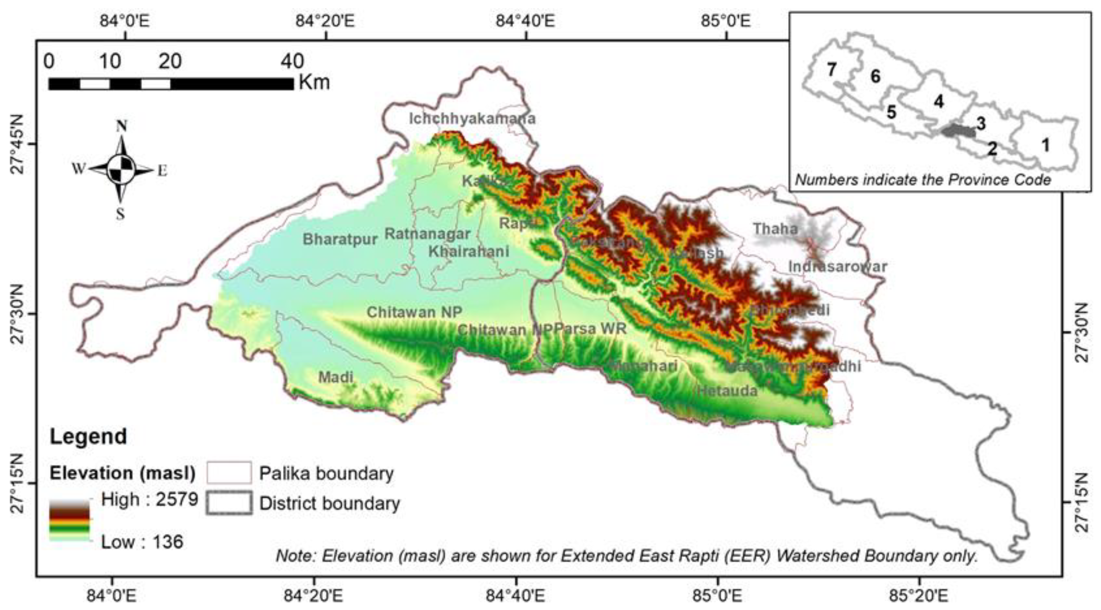
Each watershed is unique in its characteristics and the hydrological phenomenon. The fundamental science that derives hydrological processes are of course the same—however, extent of implications on streamflow alterations are expected to be different given their unique biophysical, climatic, social, and development characteristics. This paper attempts to detect the long-term changes in streamflow, their quantitative attribution to climatic and anthropogenic roots, and assess socio-economic implications in a non-snow-fed Extended East Rapti (EER) watershed located in Central-Southern Nepal (Figure 1), for which such information are not available for informed decision-making. Key research questions that the study aims to address are: (i) What are trends in rainfall and streamflow in the EER watershed? (ii) What are relative contributions of rainfall variability and anthropogenic activities towards streamflow changes? Finally, (iii) what are potential socio-environmental implications of streamflow alterations in the watershed?

2. Study Area

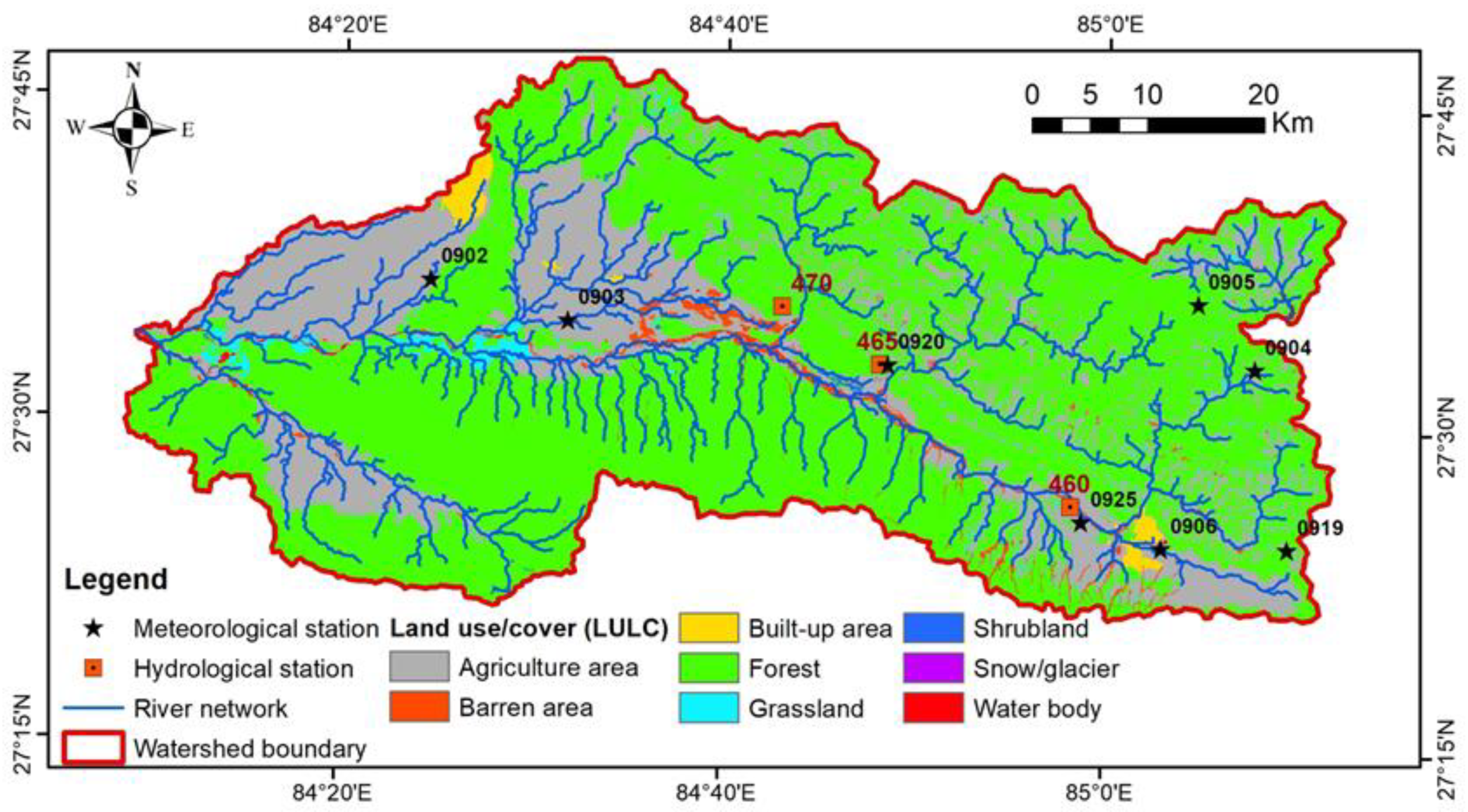
The EER watershed located in Province-3 in central-southern Nepal extends from 84.148° E to 85.206° E longitude and 27.353° N to 27.783° N latitude, (Figure 1). The total catchment area of 3202 km² above the confluence with Narayani, and including Kulekhani watershed extends over two districts, 15 Palikas (i.e., new local government units in federal Nepal), the Chitwan National Park and the Parsa Wildlife Reserve. The topography of the watershed varies from 136 to 2579 m above the mean sea level (masl). About 29.5% of the watershed area falls in the Hill and the remaining 70.5% in the Siwalik. The EER watershed has a dominance of forest (65.5%) and agricultural area (28.8%), followed by barren and grassland areas (2.1% each), built-up area (0.9%), waterbody (0.4%) and shrubland (0.2%) (Figure 2). There are two hydrological stations and eight meteorological stations in the watershed (Figure 2); two of the meteorological stations (Station-902 at Rampur and Station-905 at Daman) are climatic stations. Details of the hydro-meteorological stations in the study area are provided in

Table 1. Hydro-meteorological data and their characteristics used in the analysis.

SI	SName	Lat (N)	Lon (E)	Elev.(masl)	Data Type	River	Drainage Area (km2)	Data Period	Mean	SD	CV *	Missing Data Period
460	Rajaiya	27.442	84.971	332	Q	Rapti	443	1963–2014	27.0	6.62	0.25	Aug-Nov (1978); Jun (1982); Jul, Aug (1985); May (1990); All months in 1999; Erroneous Data in 2000
465	Manahari	27.550	84.971	305	Q	Manahari	428	1964–2015	22.4	11.96	0.53	Dec (1994); Jan, Feb (1995)
470	Lothar	27.594	84.717	336	Q	Lothar	169	1964–2015	8.9	6.26	0.70	Jan-Jun (1986); May (1990); May (2001); Aug-Dec (2004); All months in 2006; Jun-Aug (2007)
902	Rampur	27.610	84.410	256	P	-	-	1968–2017	1996.8	348.30	0.17	Few days
903	Jhawani	27.580	84.530	270	P	-	-	1968–2017	1946.2	441.71	0.23	Few days
904	Chisapani Gadhi	27.550	85.130	1706	P	-	-	1968–2017	2123.0	513.62	0.24	Dec (1995)
905	Daman	27.600	85.080	2314	P	-	-	1968–2010	1750.2	404.62	0.23	May-Jun (2003); Feb-Apr and Oct-Dec (2004); Jun, Oct-Dec (2007); Jan-May (2008); May-Jul (2010)
906	Hetauda NFI	27.410	85.050	474	P	-	-	1968–2017	2365.1	387.42	0.16	Sep-Dec (1969); All months in 1970; Jan 1971; May 1974
919	Makawanpur Gadhi	27.410	85.160	1030	P	-	-	1975–2017	2196.0	759.46	0.35	Aug-Dec (1987); Jan-Feb (2002)
920	Beluwa	27.550	84.810	274	P	-	-	1975–2016	1931.8	425.82	0.22	Few days
925	Rajaiya	27.430	84.980	332	P	-	-	1992–2014	2110.6	393.72	0.19	Jan-Feb (1992,2006); May-Dec (2007); Jun (2011); Mar-Dec (2013); Jul-Dec (2014)

Notes: SI, station index; SName, Station Name; Lat, latitude; N, northing; Lon, longitude; E, easting; Elev., Elevation; masl, meters above mean sea level; Q, discharge; P, precipitation; SD, standard deviation with units of m³/s for discharge and mm for precipitation; CV, coefficient of variation; Mean, long-term average annual value with units of m³/s for discharge and mm for precipitation. Stations 902, 905, and 906 also have daily maximum and minimum temperature records from 1968–2017 (missing years 1976 to 1979), 1973–2010 (few days missing), and 1968–2014 (few days missing), respectively.

.

Average annual rainfall in the EER watershed, based on data at eight meteorological stations, vary from 1750 mm (at st905, Daman, Elevation = 2312 masl) to 2365 mm (at st906, Hetauda NFI, Elevation = 474 masl) (Table 1). Analysis of rainfall at Rampur (Station Inde = 902) shows strong seasonality in the rainfall, with about 80% of the average annual rainfall is available only during four rainy months (June-August). Similarly, average monthly maximum temperature (Tmax) in the EER watershed varies from 22.0 °C in January to 35.9 °C in June, whereas average monthly minimum temperature (Tmin) varies from 7.7 °C in January to 25.4 °C in August.

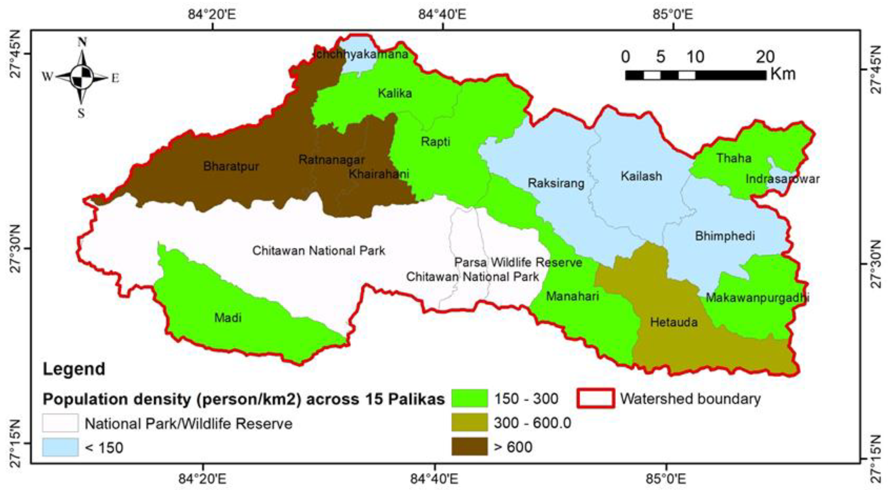
About 843.5 thousand people, with 51.01% female, are residing within the EER watershed. The population density varies across Palikas, with higher population density in the two large urban centers, such as Hetauda Sub-Metropolitan city and nearby areas, and Bharatpur Metropolitan City (Figure 3). Hetauda and Bharatpur accounts for 44.7% of the total population in the EER watershed.

3. Methods and Data

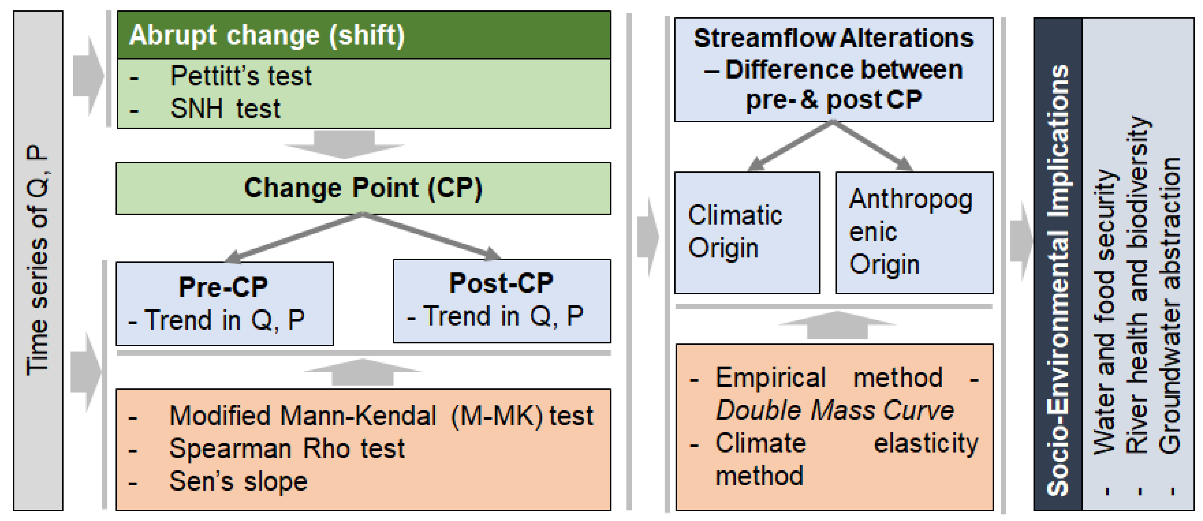
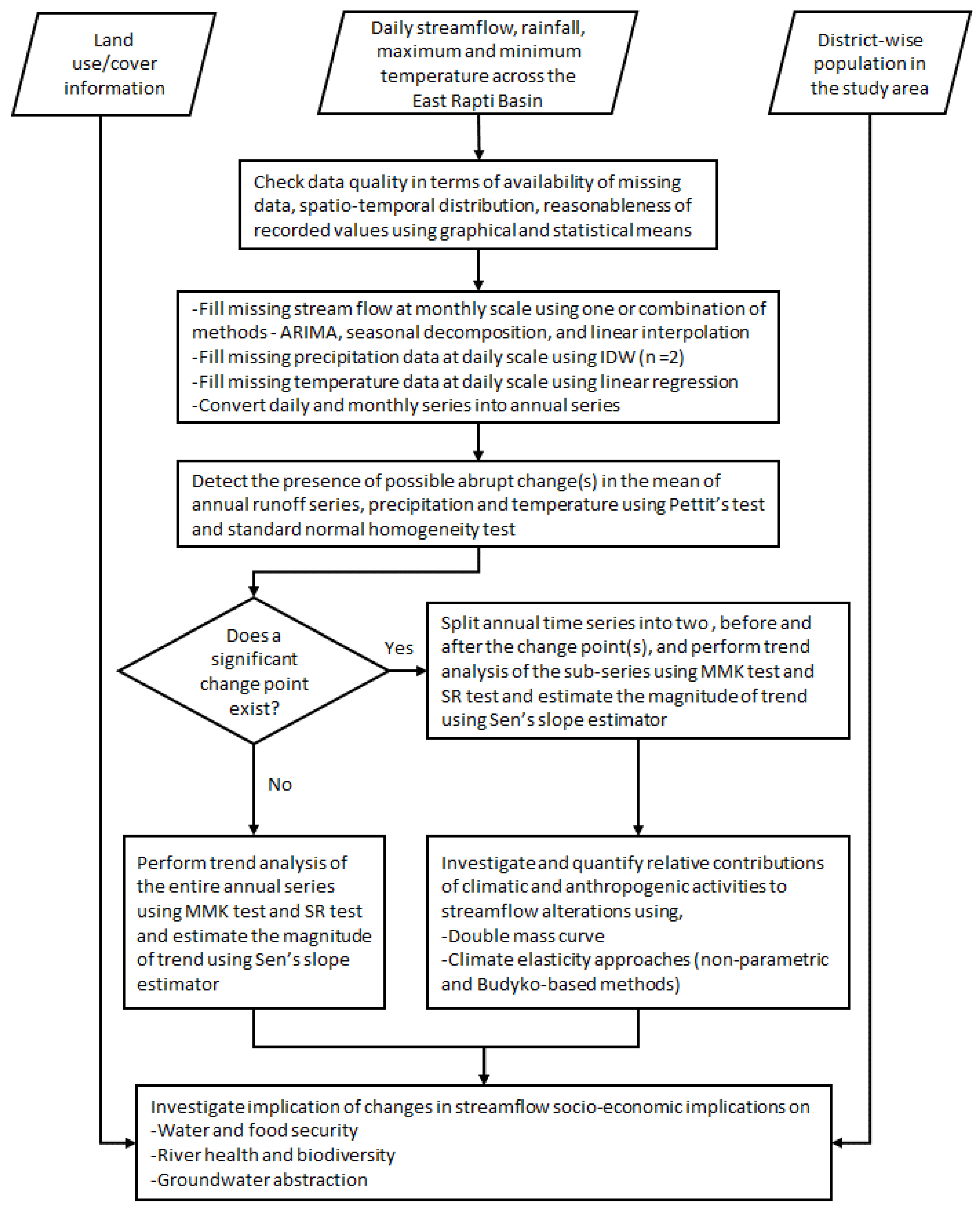
The study followed the methodological framework depicted in Figure 4, and the steps are detailed as a flow chart in Figure 5. Daily rainfall and streamflow at eight and three stations, respectively, are considered in the analysis. Key aspects of methodology, as shown in Figure 4, are described in the following subsections.

3.1. Data Collection, Screening and Pre-Processing

Observed daily time series or streamflow at three stations and rainfall at eight stations were collected as secondary data (

Table 2. Description of data used in this study and associated sources.

Data	Description	Potential Sources	Collection Method
Rainfall	Observed daily rainfall data at eight stations for the last 30 years (approximately)	DHM, Nepal	Secondary data
Hydrological data	Observed daily hydrological data at three stations for the last 30 years (approximately)	DHM, Nepal	Secondary data
Population	Current and past population data at newly formed Palikas (or earlier VDCs/Municipalities)	CBS, Nepal	Secondary data
Land use/ cover	ICIMOD (2010) or any latest products (if available)	ICIMOD (or any other sources)	Secondary data

Notes: VDC, village development committee; CBS, central bureau of statistics; ICIMOD, international center for integrated mountain development.

) from the Department of Hydrology and Meteorology (DHM), the government of Nepal. Data quality were assessed in terms of missing data and their distribution/concentration, and the reasonableness of recorded values. Data reading, hydrograph/hyetographs for different temporal scales, plot of mass curves, and comparison of means were used as an approach for assessing data quality. Finally, quality controlled data set was prepared for further analysis. Details of hydro-meteorological stations, data availability, and their characteristics, are shown in Table 1 and Table 2.

In addition to the observed hydrological and rainfall data, population and land use/cover were also collected, as mentioned in Table 2. Population data were collected from Village Development Committee (VDC) (or Palika) and then aggregated for the watershed level to estimate the basin-average population.

Annual time-series of streamflow and basin-average rainfall were generated based on daily time-series. Thiessen Polygon method was adopted for generating basin-average rainfall. Basic statistics, such as mean, median, range, quartile ranges, and coefficient of variation were calculated and analyzed for both streamflow and rainfall time-series to investigate heterogeneity in rainfall and streamflow behavior.

3.2. Dealing with Missing Data

The status of missing data in hydrological and precipitation time series is indicated in Table 2. Missing discharge data were filled using ‘imputeTS’ package in R [25]. One or combination of four methods—Kalman Smoothing, ARIMA, seasonal decomposition, and linear interpolation—depending upon their performance, were used for filling missing data for each of the three series. The method that resulted in positive discharge for the station of interest was used—therefore, methods varied as per station. For instance, at station 470, ARIMA method yielded negative discharges. Seasonal decomposition gave similar results but with few negative values on low flows month, whereas linear was not good in filling 2006 data. Hence, seasonal decomposition was chosen, but negative values were set to value of the preceding month. At station 465, except linear interpolation all other yield negative results. For station 460, ARIMA approach performed well over other methods. In the case of precipitation data, missing daily data were imputed using Inverse Weighted Distance (IDW) interpolation at daily scale with a power factor of 2.

3.3. Detection of Abrupt Shift and Gradual Shift (or Trends)

A number of studies have used change point problem in streamflow analysis for identification of time point where anthropogenic activities started to have significant alterations in magnitude of flow over the natural changes [1,22,26,27]. Basically, the process involves detection of an abrupt change point from an analysis of the statistical characteristics of a long-term hydrological series, and then further analysis like quantification of climatic and anthropogenic influences to streamflow is carried out for before and after change point series. Statistical tests, such as Pettitt’s test and standard normal homogeneity (SNH) tests, are generally carried out to detect change point. Pettitt test has the advantage of being non-parametric where the assumption of the prior distribution of data is relaxed [13]. SNH test assumes a normal distribution of data [28]. Wu et al. [22] carried out Pettitt’s test to detect an abrupt change point for observed runoff from the Yanhe River basin in China during the period 1972–2011, where after 1996, climate change played a dominant role in the decline in the runoff from the basin. Likewise, a study by Sharma et al. [1] also used Pettitt’s test, and attributed the decline in streamflow in Tapi River Basin, India to anthropogenic activities, such as changes in the land use patterns at different points of time in different tributaries of Tapi River. Likewise, SNH test has been applied to test the artificial and natural homogeneity of the average annual discharge for eight hydrological stations in the Kupa River Basin, between Slovenia and Croatia [29]. It has also been used to carry a homogeneity analysis of precipitation in Iran [30]. Due to successful application of abrupt change point method in various studies as mentioned, in this study we adopted Pettitt’s test together with SNH test [13,14,28] to detect abrupt change (or shift) in the mean of annual runoff, precipitation and temperature time series Both of these methods have been applied in order to complement each other and reinforce the analysis. The significance of the detected change point is determined using a Mann-Whitney U test [31]. Details of the method are provided in Appendix A. Data for the period of 1963–2017 was used. In the case of existence of significant change point, entire time-series was split into two, and the gradual trend was analyzed for two sub-series, before and after the change point. In the case of non-existence of significant change point, gradual shift (or trend) analysis was performed on the entire time series.

Presence of trends in streamflow time series was analyzed using non-parametric Modified Mann-Kendall (M-MK) [17], Spearman’s Rho [32] and Sen’s slope estimator [33] tests. Mann-Kendall test and Modified Mann-Kendall tests are widely used for the analysis of trends in climatic and hydrological time series [17]. Mann-Kendall test is non-parametric in nature, however it suffers from bias introduced by autocorrelation in nature. The M-MK test addresses this issue by accounting for the presence of autocorrelation in the data in addition to other advantages from the original MK test. Spearman’s Rho test, which is also non-parametric is a rank-based approach like M-MK. These tests are, therefore, not affected by distribution nature and are relatively insensitive to outliers. The magnitude of the trend was estimated using Sen’s slope estimator. The significance of the detected trend was evaluated using Spearman’s Rho test. For this study, like other similar studies on streamflow and climatic series (such as Pirnia et al. [34], Zhu et al. [7], Zhang et al. [35], Zhang et al. [36], Partal and Kahya [37]), the methods mentioned above were used though there are other approaches like segmented regression analysis, which also deals with analyzing trend of time series having change points [38]). Details on these methods are provided in Appendix A.

Furthermore, temporal trends in rainfall time-series were also performed using the same approach as used for streamflow. Spatial variation of trends in annual rainfall and runoff across the study watershed was analyzed in ArcGIS. It was basically done for rainfall data, as there was a good spatial representation of rainfall data compared to runoff data.

3.4. Attribution of Streamflow Alterations to Climatic and Anthropogenic Sources

The generic concept for this attribution is that for the catchments with streamflow not subject to any regulation, it can be modelled as a function of climatic variables and catchment characteristics. Furthermore, human factors are assumed to be independent of climatic factors. Therefore, the total change in the streamflow (ΔQ) can be expressed as a sum of ΔQ_P and ΔQ_H [22], where subscripts P and H stands for changes in streamflow, due to rainfall variability and anthropogenic (or human) activities, respectively. We also follow the approach used by Wu et al. [22] for estimating attribution of streamflow changes to climate and anthropogenic changes.

At the local scale, changes in climatic variables are independent to the human behavior shaping catchment characteristic. In the absence of any hydro-regulation, the streamflow response of a catchment can be modelled as a function of climatic variables and catchment characteristics [1]. Here, we have defined the base period (before 1990) and variation period (after 1990). Therefore, the total change in the streamflow over these two periods can be expressed as a sum of changes in streamflow, due to climatic variability and anthropogenic activities [1,22]. They are expressed as:

$$∆{\overline{Q}}_{total}={\overline{Q}}_{variation}-{\overline{Q}}_{baseline}$$

(1)

$$∆{\overline{Q}}_{total}=∆{\overline{Q}}_{climate}+∆{\overline{Q}}_{human}$$

(2)

$${\mu }_{climate}=\frac{∆{\overline{Q}}_{climate}}{∆{\overline{Q}}_{total}}\times 100\%\mathrm{and}{\mu }_{human}=\frac{∆{\overline{Q}}_{human}}{∆{\overline{Q}}_{total}}\times 100\%$$

(3)

Here, $∆{\overline{Q}}_{total}$ is the total change in the mean annual runoff between the variation period, ${\overline{Q}}_{variation}$, and the baseline period, ${\overline{Q}}_{baseline}$. $∆{\overline{Q}}_{climate}$ and $∆{\overline{Q}}_{human}$ are the changes in the mean annual runoff caused by climatic variability/change and human activities, respectively. ${\mu }_{climate}$ and ${\mu }_{human}$ are the contributions from climate variability/change and anthropogenic factors, respectively, on the runoff variation. Methods like empirical statistics (double mass curve) and elasticity-based can be applied in estimating $∆{\overline{Q}}_{climate}$ and $∆{\overline{Q}}_{human}$.

In this study, we also applied statistical approaches, such as climate elasticity [20] and double mass curve [21,22]. Their details are provided in Appendix A. After attribution to the streamflow alterations, we further discussed the linkage of attribution to changes in land use/cover and population in the study watershed.

3.5. Assessing Socio-Environmental Implications

Streamflow alterations and associated changes in water availability are linked to various aspects of society and environment; therefore, changes in streamflow is expected to have implications in the socio-environmental system. Based on the understanding of the relative contribution of rainfall variability and anthropogenic activities in streamflow changes, necessary secondary data, as well as qualitative information, were collected from various sources, including field studies commissioned during August to October, 2019. The implications were discussed from following three perspectives, which were identified as relevant for the study watersheds after field study: (i) Water and food security; (ii) river health and aquatic biodiversity; and (iii) groundwater abstraction.

4. Results and Discussion

4.1. Detection of Changes (Both Abrupt and Gradual) in Streamflow

The three hydrological stations cover approximately 32.5% of the 3202 km² large EER watershed. However, we estimated changes in streamflow in the EER watershed on the daily hydrological records at those three stations, based on the best available data. For detecting the possibility of abrupt change(s) in the average annual streamflow and precipitation series, the Pettitt and Standard Normal Homogeneity (SNH) tests were applied for selected hydrological and meteorological stations. The time period of analysis, as well as results, are tabulated in

Table 3. Results of Pettitt and standard normal homogeneity (SNH) tests for change point detection in EER watershed.

Station Index	Time Period	n	Pettitt Test: p-Value	KT	Probable Change Point/Year	Pettitt Test Result at α = 0.05	SNH Test: p-Value	Tk	Probable Change Point/year	SNH Test Result at α = 0.05
Annual Runoff
460	1963–2014	52	0.1867	238	1974	NS	0.432	4.2	1974	NS
460	1975–2014	40	0.038	208	2002	S	0.122	6.77	2002	NS
460	1975–2014 (excluding 1999 and 2000)	38	0.046	188	2002	S	0.138	6.48	2002	NS
465	1964–2015	52	0.176	241	1988	NS	0.295	5.1	1988	NS
470	1964–2015	52	0.214	231	1978	NS	0.904	1.92	2011	NS
470	1979–2015	37	0.447	114	2004	NS	0.926	1.67	2010	NS
Annual Precipitation
902	1968–2017	50	0.4579	177	1996	NS	0.5887	3.4236	2010	NS
903	1968–2017	50	0.13	241	1996	NS	0.1693	6.2395	1996	NS
904	1968–2017	50	0.01932	314	2007	S	0.0012	14.872	2007	S
905	1968–2002	35	0.7142	87	1998	NS	0.1902	5.7173	1998	NS
906	1975–2017	43	0.3976	148	2007	NS	0.4496	4.0251	2007	NS
919	1975–2017	43	0.06827	214	1988	NS	0.0801	7.616	1988	NS
920	1975–2017	43	0.05278	222	2007	NS	0.0121	10.82	2007	S
925	1992–2012	21	0.4811	48	2007	NS	0.3417	4.1944	1992	NS
Maximum Temperature
902	1968–2017	50	1.48 × 10−5	505	1982	S	<2.2 × 10−16	21.3	1982	S
905	1973–2010	38	3.43 × 10−6	353	1993	S	<2.2 × 10−16	24.25	1993	S
906	1968–2014	47	2.25 × 10−6	492	1990	S	<2.2 × 10−16	23.9	1990	S
Minimum Temperature
902	1968–2017	50	0.00028	434	1989	S	0.05	8.62	1988	S
905	1973–2010	38	0.02942	199	1993	S	0.0314	9.17	2004	S
906	1968–2014	47	0.00056	380	1983	S	0.00003	16.82	1979	S

Notes: SNH, standard normal homogeneity; S, statistically significant; NS, not significant (statistically).

, and time series are plotted in Figure 6.

Results of change point analysis showed that the majority of hydrological and precipitation stations do not exhibit abrupt changes. Statistically significant change point, at 5% level of significance, is observed only at Rajaiya hydrological station in the Rapti river (station 460) from the Pettitt test with data after 1974. Remaining two hydrological stations did not show significant change points. Likewise, these stations show non-uniformity in probable change points ranging from 1974 to 2011 (Table 3), which is very crude to consider any specific time period for change point. In the case of precipitation stations, only Chisapani Gadhi (station 904) displayed statistically significant change point, whereas the change points from other stations were statistically insignificant (Table 3). Like discharge data, they also show diversity in the occurrence of probable change points, but located after 1988. Unlike streamflow and precipitation, all temperature stations displayed significant change points during the late 1980s and early 1990s (Table 3).

For temperature signals too, these change points identified by both Pettitt’s and SNH tests are spread over a period of 1982 to 2004 (Table 3). However, it is noticeable that in majority cases, these changes are between 1982 and 1993. We take this period as a transition phase for changes in temperature for the study area. This spread of change points over a period of time have also been reported in papers like Jaiswal et al. [39] and Zarenistanak et al. [40]. Furthermore, the study area experienced a major socio-political change in 1990 that established democracy in the country. Given the local knowledge of the rise in the development process around 1990 after the democratic government started to work in full fledge, cities like Hetauda, located in the eastern part of the basin, have expanded with a boost in its economy and developed as a major economic hub after 1990. Therefore, after considering the local knowledge, as well as temperature signals, 1990 was identified as the change point for this study area. Furthermore, pre-1990 has also been designated as base-period for many climate studies and guidelines. For instance, the definition of climate change indices by the Expert Team on Climate Change Detection and Indices (ETCCDI) considers 1960–1990 period as baseline period (guidelines on analysis of extremes by the World Meteorological Organization) [41]. Moreover, methodologically, there are practices to include ‘human-designated’ approach to defined change point, and thus, the base-period [22]. We used a mixed approach that consists of looking into the hydro-climatic signal (primarily temperature in this case), as well as local stakeholders’ knowledge too, using 1990 as the change point. We, therefore, divided the entire time series of above variables into two sub-periods—the baseline period (until 1990) and the variation period (post-1990).

Then we analyzed gradual shifts (or trends) in streamflow and precipitation time series before and after the change point (i.e., 1990) in order to better understand the extent of changes in streamflow and precipitation and their linkages (if any). We analyzed trends using M-MK approach, computed Sen’s slope and tested its significance using M-MK and Spearman’s rho statistics.

Table 4. Streamflow and precipitation trends in Extended East Rapti (EER) watershed.

SI	Time Period	Type+	n	MMK-Z Statistic after Variance Correction	M-MK-P-Value after Variance Correction	Original MK Z Statistic	Original Mann-Kendall p-Value	Mann-Kendall’s Tau	Sen’s Slope (m³/sec /Year)	Spearman Correlation Coefficient Value	Z-Transformed Test Statistic	Spearman Test p-Value	Significance of M-MK (at α= 0.05)	Significance-Spearman’s Rho Test (at α = 0.05)
Discharge/Streamflow
460	1963–2014	O	52	−0.33	0.741	−0.481	0.63	−0.047	−0.027	−0.08	−0.573	0.567	NS	NS
460	1963–1990	O	28	−1.205	0.228	−1.205	0.228	−0.164	−0.181	−0.221	−1.149	0.251	NS	NS
460	1991–2014	O	24	3.001	0.003	3.001	0.003	0.442	0.467	0.626	3.003	0.003	S	S
465	1964–2015	O	52	0.923	0.356	0.923	0.356	0.089	0.062	0.135	0.965	0.334	NS	NS
465	1964–1990	O	27	−0.917	0.359	−0.917	0.359	−0.128	−0.189	−0.183	−0.934	0.35	NS	NS
465	1991–2015	O	25	−0.49	0.624	−0.49	0.624	−0.073	−0.097	−0.135	−0.663	0.507	NS	NS
470	1964–2015	O	52	−8.181	0	−2.328	0.02	−0.223	−0.073	−0.303	−2.162	0.031	S	S
470	1964–1990	O	27	−1.376	0.169	−1.376	0.169	−0.191	−0.12	−0.218	−1.111	0.266	NS	NS
470	1991–2015	O	25	−1.452	0.146	−0.911	0.362	−0.133	−0.054	−0.22	−1.078	0.281	NS	NS
Precipitation
902	1968–2017	O	50	0.276	0.783	0.351	0.725	0.035	1.374	0.039	0.276	0.783	NS	NS
902	1968–1990	O	23	−0.951	0.342	−0.951	0.342	−0.146	−8.815	−0.187	−0.876	0.381	NS	NS
902	1991–2017	O	27	−0.208	0.835	−0.208	0.835	−0.031	−2.567	−0.076	−0.386	0.699	NS	NS
903	1968–2017	O	50	0.825	0.41	1.004	0.315	0.099	4.755	0.155	1.084	0.278	NS	NS
903	1968–1990	O	23	0.528	0.597	0.528	0.597	0.083	7.86	0.12	0.561	0.575	NS	NS
903	1991–2017	O	27	0.208	0.835	0.208	0.835	0.031	3.085	0.049	0.249	0.803	NS	NS
904	1968–2017	O	50	−1.245	0.213	−1.522	0.128	−0.149	−8.531	−0.254	−1.78	0.075	NS	NS
904	1968–1990	O	23	−0.898	0.369	−0.898	0.369	−0.138	−15.506	−0.233	−1.094	0.274	NS	NS
904	1991–2017	O	27	−1.418	0.156	−1.418	0.156	−0.197	−24.986	−0.375	−1.911	0.056	NS	NS
905	1968–2002	O	35	0.398	0.691	0.398	0.691	0.049	2.85	0.099	0.575	0.565	NS	NS
905	1968–1990	O	23	0.233	0.815	0.317	0.751	0.051	5.5	0.079	0.371	0.711	NS	NS
905	1990–2002	O	13	0.915	0.36	0.915	0.36	0.205	54.883	0.374	1.294	0.196	NS	NS
906	1975–2017	O	43	0.213	0.831	0.314	0.754	0.034	1.767	0.031	0.2	0.842	NS	NS
906	1975–1990	O	16	1.216	0.224	1.216	0.224	0.233	15.567	0.312	1.207	0.227	NS	NS
906	1991–2017	O	27	−0.125	0.9	−0.167	0.868	−0.026	−1.62	−0.048	−0.246	0.806	NS	NS
919	1975–2017	O	43	0.375	0.708	0.649	0.516	0.07	6.49	0.086	0.56	0.576	NS	NS
919	1975–1990	O	16	−0.099	0.921	−0.135	0.893	−0.033	−17.075	−0.126	−0.49	0.624	NS	NS
919	1991–2017	O	27	−1.811	0.07	−2.377	0.017	−0.328	−45.125	−0.512	−2.609	0.009	NS	S
920	1975–2017	O	43	−2.293	0.022	−1.695	0.09	−0.181	−9.305	−0.268	−1.74	0.082	S	NS
920	1975–1990	O	16	−1.396	0.163	−1.396	0.163	−0.267	−21.736	−0.397	−1.538	0.124	NS	NS
920	1991–2017	O	27	−1.108	0.268	−1.251	0.211	−0.174	−15.28	−0.275	−1.401	0.161	NS	NS
925	1992–2012	O	21	−0.617	0.537	−0.755	0.45	−0.124	−10.618	−0.16	−0.714	0.475	NS	NS

Notes: O, series with filled values, * NS, not significant; S, significant at α = 0.05; Statistically significant series are highlighted in grey; SI, station index; statistically significant trends are shaded.

and Figure 6 shows the results of the trend analysis. Lothar Khola hydrological station (station 470) exhibit a significant decreasing trend in streamflow during 1964–2017 at the rate of 0.073 m³/s/year. Although trends before and after 1990 both decrease, they are not statistically significant. In contrast, streamflow at Rajaiya (station 460) shows a significant increasing trend after 1990, at a rate of 0.467 m³/s/year, but the trend for the entire series during 1963–2017 decreases (not significant). The increase after 1990 is attributed to diversion of water from Kulekhani watershed to East Rapti during operation of Kulekhani hydropower project, which came into operation in the late 1980s. Furthermore, the Rajaiya station is just downstream of Hetauda municipality, the urban center. Streamflow at Manahari (station 465) show decreasing trends both before and after a990, but they are statistically insignificant.

In the case of precipitation, it is interesting that except stations 919 and 920 during periods 1991–2017 and 1975–2017 none of the precipitation time series have statistically significant trends. Station 920 records show a decrease (significant) of approximately 9.3 mm of precipitation per year during 1975–2017, while after 1990 rate of decrease is only 15 mm/year (insignificant). After 1990, stations 903 and 905 show positive trend in precipitation (insignificant), while we observed a decreasing trend of precipitation at other stations. The highest rate of decrease in precipitation after 1990 is observed at station 919 at the rate of approximately 45 mm per year (significant for Spearman’s rho test, but insignificant for M-MK test). Likewise, the highest rate of increase (55 mm/year, approximately) in precipitation is observed at station 905. Trend analysis for temperature series are presented in Appendix B.

4.2. Relative Contributions of Climatic and Anthropogenic Activities to Streamflow Alterations

We partitioned streamflow changes to climatic and human factors using double mass curve (DMC) and climate elasticity methods. The entire time series was divided into baseline (up to the change point, i.e., 1990) and variation (post-1990) periods (

Table 5. Proportional impacts of climate change and human activities on runoff reduction in the Extended East Rapti watershed, estimated by double mass curve method.

Index	Period	Reconstruction Equation	Observed average Annual Streamflow (mm)	Change (mm)	Reconstructed Average Annual Streamflow (mm)	Human Activities-Induced Change; mm (%)	Climate Change-Induced Change; mm (%)
460	Baseline	$Q_{cum}^{\ast }=0.891\ast x+1480.6$	1974.6	-	-	-	-
	Variation		1887.5	−87.1	1959.1	−71.6 (82.2)	−15.5 (17.8)
465	Baseline	$Q_{cum}^{\ast }=0.6411\ast x+526.1$	1342.2	-	-	-	-
	Variation		1991.0	+648.8	1269.3	+721.7 (111.2)	−72.9 (−11.2)
470	Baseline	$Q_{cum}^{\ast }=0.8568\ast x+470.1$	1716.0	-	-	-	-
	Variation		1460.7	−255.2	1716.8	−256.1 (100.4)	+0.8 (−0.4)

). DMC, a non-parametric method, uses the long-term relationship between precipitation and streamflow, and provide streamflow response to precipitation. However, it does not take the physical processes into consideration. DMC reconstructs the cumulative annual streamflow (and thus, annual streamflow) in variation period using regression parameters from the baseline period, forced by precipitation in variation period. Thus, the difference in observed mean streamflow in variation period and reconstructed streamflow gives the contribution by the human activities. Results of DMC analysis indicated that human activities are the dominant cause of a decrease in streamflow at stations 460 and 470, and an increase in streamflow at station 465 (Table 5). At stations 460 and 470, they account for 82.2% and 100.4% decrease respectively. The excess 0.4% of the volume is added to the streamflow by rainfall variability/ change (i.e., climate change contribution) at station 470. The increase in streamflow at station 465 is unrealistic as there are no notable human activities and/or water inflow from other systems to the station 465 watershed were identified during the field study. Further diagnosis revealed that observed streamflow at the station 465 for the 2002 and 2003 are 70.83 m³/s and 73.71 m³/s, respectively, which are 2.7 times higher than the long-term average in the same watershed. Since we could not get an adequate basis to drop data of those two years, it influenced overall trends. Therefore, the results of station-465 should be used cautiously. In overall, results from the empirical statistical method, DMC, reveals that human activities have played a leading role in altering streamflow after the 1990s.

We also assessed the impacts of human activities and climate change on streamflow using Budyko hypothesis, an elasticity-based method.

Table 6. Climate elasticity for streamflow and proportional impact of climate change on streamflow changes in the EER watershed.

Methods	$∆\overline{\mathit{P}}$	$∆\overline{\mathit{Q}}$	$∆{\overline{\mathit{E}\mathit{T}}}_0$	${\mathit{\epsilon }}_{\mathit{p}}$	${\mathit{\epsilon }}_{\mathit{E}\mathit{T}0}$	$∆{\overline{\mathit{Q}}}_{\mathit{c}\mathit{l}\mathit{i}\mathit{m}\mathit{a}\mathit{t}\mathit{e}}^{\mathit{P}}$	$∆{\overline{\mathit{Q}}}_{\mathit{c}\mathit{l}\mathit{i}\mathit{m}\mathit{a}\mathit{t}\mathit{e}}^{\mathit{E}\mathit{T}0}$	$∆{\overline{\mathit{Q}}}_{\mathit{c}\mathit{l}\mathit{i}\mathit{m}\mathit{a}\mathit{t}\mathit{e}}$	$∆{\overline{\mathit{Q}}}_{\mathit{h}\mathit{u}\mathit{m}\mathit{a}\mathit{n}}$	$∆{\overline{\mathit{Q}}}_{\mathit{c}\mathit{l}\mathit{i}\mathit{m}\mathit{a}\mathit{t}\mathit{e}}\left(\mathit{\%}\right)$	$∆{\overline{\mathit{Q}}}_{\mathit{h}\mathit{u}\mathit{m}\mathit{a}\mathit{n}}\left(\mathit{\%}\right)$	Remark
Station 460—East Rapti sub-watershed
Sankarasubramanian et al. [42]	81.1	−87.1	80.9	0.267	−0.940	19.5	−101.8	−82.3	−4.8	94.5	5.5
Zheng et al. [20]	81.1	−87.1	80.9	0.328	−0.753	23.9	−81.5	−57.6	−29.5	66.1	33.9
Schreiber [43]	81.1	−87.1	80.9	1.673	−0.673	122.2	−72.9	49.3	−136.4	−56.7	156.7
Ol’dekop [44]	81.1	−87.1	80.9	2.075	−1.075	151.6	−116.4	35.2	−122.3	−40.4	140.4
Budyko [45]	81.1	−87.1	80.9	1.838	−0.838	134.2	−90.7	43.6	−130.7	−50.0	150.0
Pike [46], Turc [47]	81.1	−87.1	80.9	1.870	−0.87	136.6	−94.2	42.4	−129.5	−48.7	148.7
Fu et al. [48]	81.1	−87.1	80.9	1.995	−0.995	145.8	−107.8	38.0	−125.1	−43.6	143.6	m = 3
Zhang et al. [49]	81.1	−87.1	80.9	1.743	−0.743	127.3	−80.4	46.9	−134.0	−53.8	153.8	w = 1
Station 465—Manahari river sub-watershed
Sankarasubramanian et al. [42]	−12.2	648.8	69.5	0.821	−0.252	−8.5	−20.9	−29.4	678.2	−4.5	104.5
Zheng et al. [20]	−12.2	648.8	69.5	0.834	−0.915	−8.7	−75.9	−84.6	733.4	−13.0	113.0
Schreiber [43]	−12.2	648.8	69.5	1.714	−0.714	−17.8	−59.2	−77.0	725.8	−11.9	111.9
Ol’dekop [44]	−12.2	648.8	69.5	2.132	−1.132	−22.1	−93.8	−116.0	764.8	−17.9	117.9
Budyko [45]	−12.2	648.8	69.5	1.883	−0.883	−19.6	−73.2	−92.8	741.6	−14.3	114.3
Pike [46], Turc [47]	−12.2	648.8	69.5	1.918	−0.918	−19.9	−76.2	−96.1	744.9	−14.8	114.8
Fu et al. [48]	−12.2	648.8	69.5	2.058	−1.058	−21.4	−87.7	−109.1	757.9	−16.8	116.8	m = 3
Zhang et al. [49]	−12.2	648.8	69.5	1.779	−0.779	−18.5	−64.6	−83.1	731.9	−12.8	112.8	w = 1
Station 470—Lothar Khola sub-watershed
Sankarasubramanian et al. [42]	7.0	−255.2	62.7	1.149	−1.815	6.4	−122.5	−116.1	−139.1	45.5	54.5
Zheng et al. [20]	7.0	−255.2	62.7	1.077	−1.904	6.0	−128.5	−122.5	−132.7	48.0	52.0
Schreiber [43]	7.0	−255.2	62.7	1.744	−0.744	9.8	−50.2	−40.5	−214.7	15.9	84.1
Ol’dekop [44]	7.0	−255.2	62.7	2.171	−1.171	12.2	−79.1	−66.9	−188.3	26.2	73.8
Budyko [45]	7.0	−255.2	62.7	1.916	−0.916	10.7	−61.9	−51.1	−204.1	20.0	80.0
Pike [46], Turc [47]	7.0	−255.2	62.7	1.954	−0.954	11.0	−64.4	−53.4	−201.8	20.9	79.1
Fu et al. [48]	7.0	−255.2	62.7	2.103	−1.103	11.8	−74.5	−62.7	−192.5	24.6	75.4	m = 3
Zhang et al. [49]	7.0	−255.2	62.7	1.806	−0.806	10.1	−54.4	−44.3	−210.9	17.4	82.7	w = 1

Note: Aridity index for East Rapti, Manahari, and Lothar Khola sub-watersheds are 0.673, 0.714 and 0.744, respectively. ‘m’ and ‘w’ are model parameters relating to catchment characteristics in Fu et al. [48] and Zhang et al. [49] models.

shows for three sub-watersheds in the EER watershed, the climate elasticity for runoff (i.e., the precipitation elasticity for runoff (${\epsilon }_P$)) and the potential evapotranspiration elasticity for runoff (${\epsilon }_{ET0}$) were estimated from eight water-balance models, two based on nonparametric methods, and six based on the Budyko hypothesis. As shown in Table 6, the ${\epsilon }_P$ ranged from 0.267 to 2.075 for the East Rapti sub-watershed (Inde = 460), from 0.821 to 2.132 for Mahahari sub-watershed (station 465) and from 1.077 to 2.171 for Lothar Khola sub-watershed. Likewise, the ${\epsilon }_{ET0}$ ranged from −1.075 to −0.673 for East Rapti, −1.132 to −0.252 for Mahahari and from −1.904 to −0.806 for Lothar Khola. These results, for the East Rapti sub-watershed, indicate that a 1% change in precipitation will result in a 0.267% to 2.075% change in the runoff, a 1% increase in potential evapotranspiration will lead to a 1.075% to 0.673% decrease in the runoff. There were differences in the estimates of elasticity coefficients among the eight methods. Studies, such as Sankarasubramanian et al. [42] and Zheng et al. [20], estimate that the precipitation elasticity for runoff (${\epsilon }_P$) is lower in comparison to the estimations from the Budyko hypothesis. However, evapotranspiration elasticity for runoff (${\epsilon }_{ET0}$) estimates for non-parametric approaches have similar values with estimates from the Budyko hypothesis. It is to be noted that aridity index for East Rapti, Manahari, and Lothar Khola sub-watersheds are 0.673, 0.714, and 0.744, respectively, implying that basin is humid.

The influence of climate change and human activities on streamflow alteration as calculated by different climate elasticity methods are shown in Table 6. For the East Rapti sub-watershed, non-parametric methods and the Budyko hypothesis showed two contrasting results. Non-parametric methods showed that climate change-induced runoff declined by 57.6 to 82.3 mm, which accounts to 66.1 to 94.5% of total change, and we notice that evapotranspiration played a major role in this decline. In contrast, the Budyko hypothesis attributed the climate factor for the addition of runoff by 38 mm to 49.3 mm, while human factor reduced runoff by 125.1 to 136.4 mm; thus, with a net effect of reduction of runoff. From the field study, it is clearly seen the anthropogenic activities are the major reason for alterations in streamflow. In the Manahari river sub-basin, runoff is reduced by 29.4 to 93.8 mm, due to climate effects, both precipitation and evapotranspiration leading to a reduction in the runoff. In the Lothar Khola sub-watershed, non-parametric approaches yield similar magnitude of decrease in the runoff (45.5% to 48% by climate factor and 54.5% to 52% by an anthropogenic factor) in the basin. In contrast, Budyko hypothesis-based method showed that the influence of climate change is limited to 15.9% to 24.6 % only, the rest (75.4% to 84.1%) is due to the human factor.

In a nutshell, human activities are playing a dominant role in altering, more specifically, decreasing streamflow after 1990 in the EER watershed. Climate change is also contributing to alterations in streamflow, but less dominantly compared to anthropogenic activities, and contribution of evapotranspiration is significant in climate change-induced alterations.

4.3. Socio-Environmental Implications of the Streamflow Changes

Alterations in streamflow have implications in various sectors. Growing population (Appendix C), urbanization (eight out of 15 Palikas in EER watershed are Municipalities), land use/cover changes (Appendix D) and climate change/variability, among others, are contributing to alterations in streamflow. As a result, there are implications on water availability and food security, river health and aquatic biodiversity, and groundwater abstraction, among others.

4.3.1. The Implication to Water and Food Security

The EER watershed is home for nearly 765,000 populations [50] distributed across 15 Palikas with varying densities (Figure 5). In Chitwan district, which covers nearly 55% of the EER watershed area, the population has increased by 123% during 1981–2011 (Appendix C). Furthermore, feeding to the growing population needs more food production, and most of the irrigation water for food production is withdrawn from rivers within the EER watershed.

As per the National Irrigation Master Plan [51], Chitwan district currently has 20,643 ha of irrigated land through 53 irrigation projects, which is nearly half of total irrigable areas of 42,000 ha. Similarly, in Makwanpur district, out of 23,500 ha of irrigable areas, only 2406 ha are covered by irrigation through 33 irrigation projects. Therefore, with a future emphasis of all the three-tier governments on intensifying agricultural activities to feed a growing population, more irrigation coverage is expected in near to mid-future. With more increase in irrigated areas and associated water use coupled with altered streamflow, crop production and food security are likely to get affected unless climate-resilient agricultural practices are put in place. The alterations in streamflow either from climatic or anthropogenic origin can introduce new challenges for watershed-level management of water resources, and more specifically, transboundary water management in the EER watershed, which are shared by 15 local governments in the new federal governance structure of Nepal.

From the analyses presented in Section 4.1, it is clearly seen that the EER watershed exhibits a decreasing trend in streamflow post-1990. The persistence of such trends in the near future would potentially escalate the water crisis and conflicts in the watershed. Thus, rapidly increasing population and declining freshwater availability may affect the food grain production, which would likely manifest food shortages in the area.

Agricultural areas in the Chitwan and Makwanpur districts in the EER watershed have increased from 28.5% to 29.7%, and from 19.7% to 22.2%, respectively, during 2000 to 2010 (Appendix D), which have manifested an increase in irrigation water requirements. The annual production of main crops (i.e., paddy, wheat, maize, and millet) have increased in general in both the districts that share the EER watershed (

Table 7. Trends in annual crop production (metric tons) in the EER watershed districts (Source: References [54,55,56]).

Crop	District	2010/2011	2013/2014	2016/17
Paddy	Makwanpur	36,630	38,381	41,458
Wheat	Makwanpur	11,796	12,007	12,980
Maize	Makwanpur	40,456	67,870	68,759
Millet	Makwanpur	3206	3280	3251
Paddy	Chitwan	110,944	100,555	108,996
Wheat	Chitwan	26,533	29,899	22,119
Maize	Chitwan	52,463	29,250	19,250
Millet	Chitwan	1868	1600	1490

). The rising trend in the production of water-intensive crops, such as paddy, is further posing stress on available water resources in the watershed. It would further be aggregated by land use/cover change in the watershed. Though there are no data available on land use/cover change trends, as well as future projections to quantify impacts, a general tren is the decrease in forest areas as in other regions of Chure belt in Nepal, decrease in open areas, and increase in built-up areas in and around the urban centers. This phenomenon has socio-economic implications in terms of increase in intensity and frequency of flash floods, deterioration of water quality, and decrease in recharge to groundwater aquifers, among others; all of which have implications on water (quantity, quality, and timing). Projecting future land use/cover and quantifying the extent of impacts on the aforementioned aspects of water could be considered as a next step for furthering this research.

Alterations in streamflow may affect the production of paddy and other crops and therefore have implications in food security. Interactions with locals in the watershed further confirm that changes in agricultural areas are already a reality. Due to declining water availability, farmers are resorting to growing crops like maize that require less water than growing water-intensive crops or leaving the land fallow altogether. The impact is further exacerbated, due to the fact that many farmers practice subsistence agriculture, and few are sharecroppers.

On the other hand, the alarming rise in population (e.g., a 123% increase during 1981–2011 in Chitwan district) has manifested an increase in water and food demands. Availability of edible food (defined here as rice, maize, wheat, barley and buckwheat) has decreased from 87,662 metric tons (MT) in 2011/12 to 67,448 MT in 2014/15 in Makwanpur district [52,53]. Similar trends are observed in Chitwan district as well; a reduction from 86,581 MT to 22,875 MT for the same period. As the population is growing at the rate of 2.3% in the area, the per capita food availability (kg/yr) during the period is also certainly decreasing. Though the quantitative impact of water stress conditions on per capita food availability could not be ascertained (due to lack of data), it is highly likely. If it persists for longer period, it may lead to food insecurity in the watershed.

To ensure food security and avert a crisis in the future, strategies for water demand management (e.g., efficient irrigation methods, develop and practice climate-adaptable crop varieties, etc.), as well as supply side management (e.g., practice rain water harvesting, implement water conservation measures, such as efficient recycle and reuse of water, educate and raise awareness of users on water conservation, etc.), need to be devised. Moreover, implementation structures need to be put in place, and monitoring and evaluation of effective implementation must be carried out.

4.3.2. The Implication to River Health and Aquatic Biodiversity

Healthy rivers have the potential to provide surrounding communities with a variety of benefits. Streamflow regime plays a key role in shaping the structure and health of water environments [57]. Alteration in the natural flow regime, due to interventions on water and land resources, can impact adversely on riverine ecology, morphology, riparian rights of the downstream users, and downstream water environments [1,58]. Land use/cover change in the form of deforestation may contribute to the degradation of landscape, soil erosion and sedimentation, which have adverse implications to river health and aquatic biodiversity. Furthermore, change in the river regime as a result of land use/cover change may affect the growth and reproduction of some flora and fauna in the riverine ecosystem. Other aspects of land use/cover change, such as urbanization, may contribute to flash floods and the subsequent change in flow regime, as well as the discharge of polluted water directly to the freshwater system, which can disrupt natural environments and degrade ecosystems [59,60]. This phenomenon can ultimately cause irreversible consequences for both human and ecosystems [61]. Therefore, alterations in water availability, but increasing water demands in the EER watershed will increase competitions between human use and environmental needs, which further affects adversely to river health and aquatic biodiversity.

The decreasing streamflow in the study area has deteriorated capacity of rivers to dilute pollutants, due to excessive use of chemical fertilizers and pesticides in agricultural lands and industrial pollutions generated from at least 134 various types of industries [62] in the Hetauda Industrial District. Therefore, river systems are more polluted than before, even though there are no studies to quantify the extent of degradation in river health. As more industrial districts (e.g., Shaktikhor in Chitwan and Mayurdhap in Makwanpur [63], etc.) are planned in the EER watershed, if industrial wastewater is not pre-treated before disposing to the river, it will certainly affect negatively to aquatic biodiversity. Washing of vehicles in the river, which is widespread in the East Rapti River, and associated mixing of automobile chemicals will have impacts on aquatic flora and fauna, which are not yet all studied. In addition, riverbed mining, which is widespread in the EER watershed, is also affecting adversely to river ecology, river health, and aquatic biodiversity. There is also a hypothesis that recent cases of deaths of over 40 rhinos in the Chitwan National Park, as well as the decline in fish production in Markhu, Kulekhani over the decade, could potentially be linked to the deteriorated water quality of the rivers as one of the causes, though there is no proof so far.

In a nutshell, although there are no scientific studies to quantify them, anthropogenic activities (such as industrialization, intensified agriculture, and urbanization) are degrading river health, and affecting adversely to aquatic biodiversity in the EER watershed. Moreover, they may also accelerate the eutrophication in water bodies through an increase in the rate of nutrient inputs draining into the streams. Alteration in streamflow coupled with extensive eutrophication, may affect adversely the already degraded self-purification capacity of the river system, degrades water quality, and pose a threat to the aquatic flora and fauna. Therefore, a cooperation framework among local riparian governments for managing the shared EER watershed could be the potential pathway for the prosperity of the local governments, as well as of the watershed. The framework, from the perspective of maintaining river health and preserving aquatic biodiversity, could potentially be operationalized by introducing the concept of Environmental Flow (E-flows) and ensuring commitments of all the local governments to comply with that. As new governments are ready to frame their development strategies, it is the right time to introduce this intervention for ensuring healthy rivers, maintenance of aquatic biodiversity, and sustaining human life for a long run.

4.3.3. Implications on Groundwater Abstraction

It is estimated that population growth in the EER watershed has increased domestic water demand alone by 140%, during 2011–2019, which is projected to increase further by 2050. Furthermore, need for food, energy and other resources for the increased population has resulted in an increase in agricultural areas over the past decades (Appendix D). The trend is expected to increase further in future, in order to cater for more food for growing population. This will have implications in water demand. As identified in the field study carried out during October 2019, average duty in the study area is 2 L per second (lps) per hectare in the study area. It means that per hectare increase in the irrigated area increases water demand by 2 lps. In this context, given relatively flat topography of the EER watershed (about 33% of the EER watershed lying in Tarai, i.e., at the elevation below 300 m) and availability of groundwater resources, pressure on the precious groundwater resources are likely to increase. Domestic and agricultural activities in various locations within the EER watershed are critically dependent on groundwater resources. About 46% of the water used by households in the watershed for drinking purpose is abstracted through groundwater sources [50]. Potentially declining groundwater levels, coupled with alterations of streamflow, is expected to have an impact on domestic uses, as well as food security. If the groundwater abstraction is not regulated properly, groundwater resources are likely to deplete, though there are no scientific estimates on groundwater recharge, the current level of groundwater abstraction, and potential impacts of an increase in water demand. For example, Hetauda Sub-Metropolitan City (HSMC) area alone has nearly 25 tubewells with depths and discharge varying in a range of 76–105 m and 5–32 lps, respectively, are drilled during 2004–2009 (Source: Personal communication with Groundwater Resources Development Board, Chitwan in September 2019) to abstract groundwater for irrigation. Furthermore, the Irrigation Master Plan [51] has included Chitwan as one of the priority districts for groundwater projects. These trends are expected to continue to cater to water demands in the EER watershed for domestic, irrigation, industrial, and other purposes.

Urban pockets in the EER watershed, such as HSMC, Bharatpur Municipality, and others, are expected to abstract more groundwater resources while moving farther in the future, thus exerting more pressure on the precious resource Population in the HSMC areas grew at the rate of 2.6%, but urban areas increased by four-fold during 1995–2011 [64], which is continuing to increase after it became a sub-metropolitan city with the recent change in the governance structure of the country to federal. Water-intensive lifestyle in urban areas, which are getting supply mostly from groundwater, is already adding more pressure on groundwater resources through increased abstraction. Groundwater production by Hetauda Water Supply Management Board (HWSMB) has increased by 25% during 2016–2018 to supply water for the HSMC dwellers. Furthermore, groundwater abstraction as the major source of irrigation supply in the vast majority of agriculture areas is expected to continue for, at least, the foreseeable future. In the context of further alterations in surface water, groundwater abstraction would further be accelerated as a safe and reliable source of water supply for various uses in the parts of the watershed where feasible. On the other hand, land use/cover change in the form of urbanization has decrease open and cultivation areas in the HSMC area, which recharge the groundwater system, by at least 7% during 1995–2011 [64], which affects adversely to recharge and then to groundwater availability. Though there is no detailed mapping of groundwater potential and aquifer depths in the EEER watershed, groundwater aquifer in the flat southern part of the watershed is expected to be a single unconfined aquifer with about 200 m thickness in HSMC areas with variation in depth across the watershed. The static groundwater level in the HSMC area is at a depth of 10–58 m below the ground surface, and groundwater in the area is being abstracted from nearly 25 wells to cater for nearly 86% of the water demand in the HSMC (source: Authors analysis based on secondary information collected during a field visit in 2019). All these scenarios reflect continued increase groundwater abstraction in the future.

From interaction with stakeholders during a field visit in mid-2019, it was noted that groundwater levels in a couple of wells were depleted over the years. As new governments are keen to do something new to contribute to the prosperity of their constituency, it is likely to put more pressure on groundwater resources, but it is not well understood and represented to inform decision-making. In overall, increase in industrial and urbanization activities and continued need of water for agricultural intensification to fuel food security is expected to impact adversely to groundwater levels in parts of the EER watershed. Furthermore, lowering groundwater levels will likely reduce groundwater contribution to natural streams, which will further contribute to declining streamflow across the basin. Therefore, a baseline study for stock-taking of the current state of groundwater availability, withdrawal, recharge, and estimates on the allowable level of groundwater abstraction would be helpful for strategically using groundwater resources, without conflict with adjoining local governments, for the prosperity of the EER watershed.

5. Conclusions

This study, regarding the Extended East Rapti (EER) watershed in central-southern Nepal, evaluated trends in rainfall and streamflow, estimated relative contributions of rainfall variability and anthropogenic activities towards streamflow changes, and discussed potential socio-environmental implications of the streamflow alterations. Key conclusions from the analysis are:

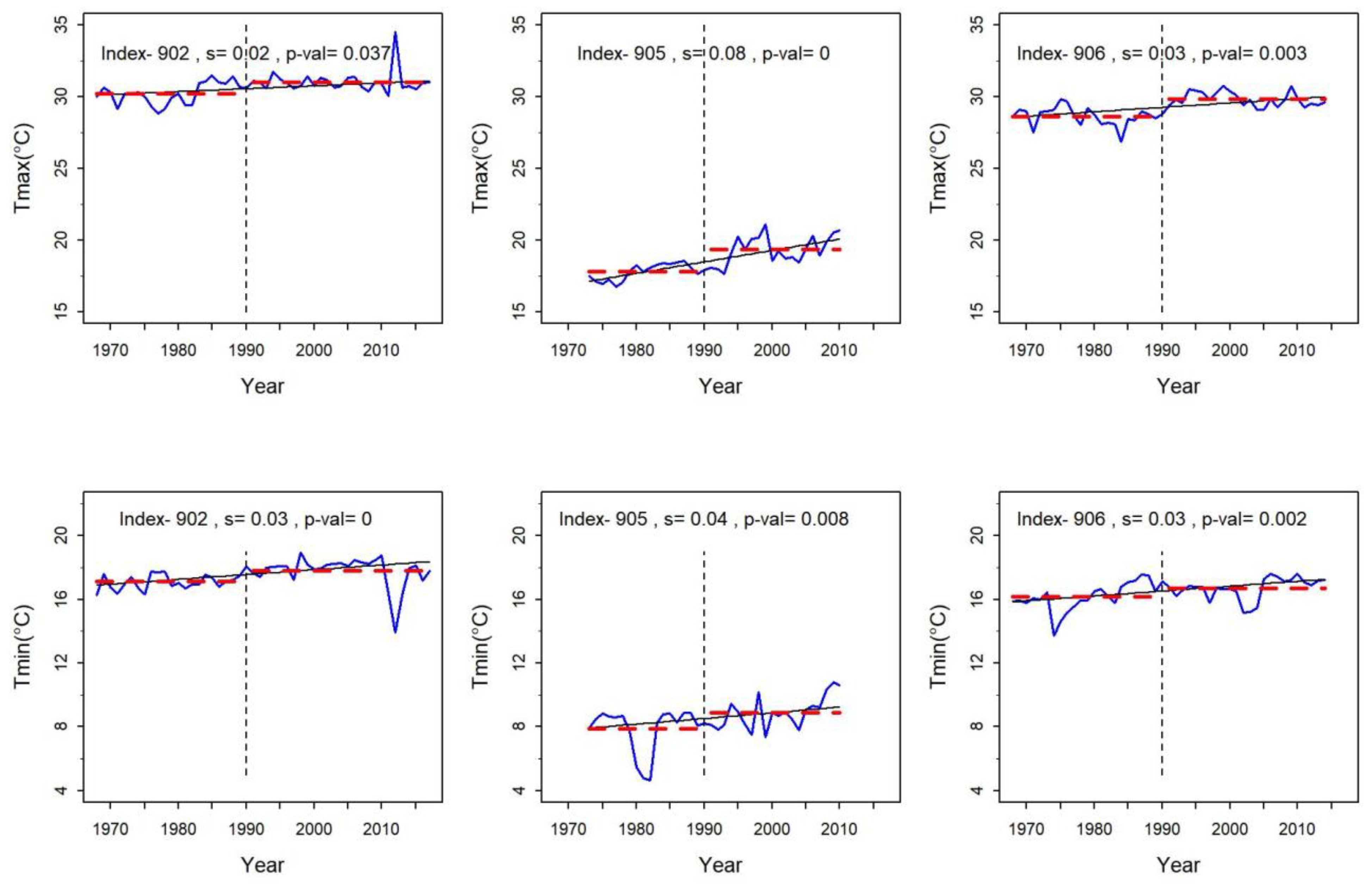
• Two distinct trends in hydro-climatic time series (temperature) exist before and after 1990. Therefore, 1990 can be considered as the change point for the abrupt change in the EER watershed.
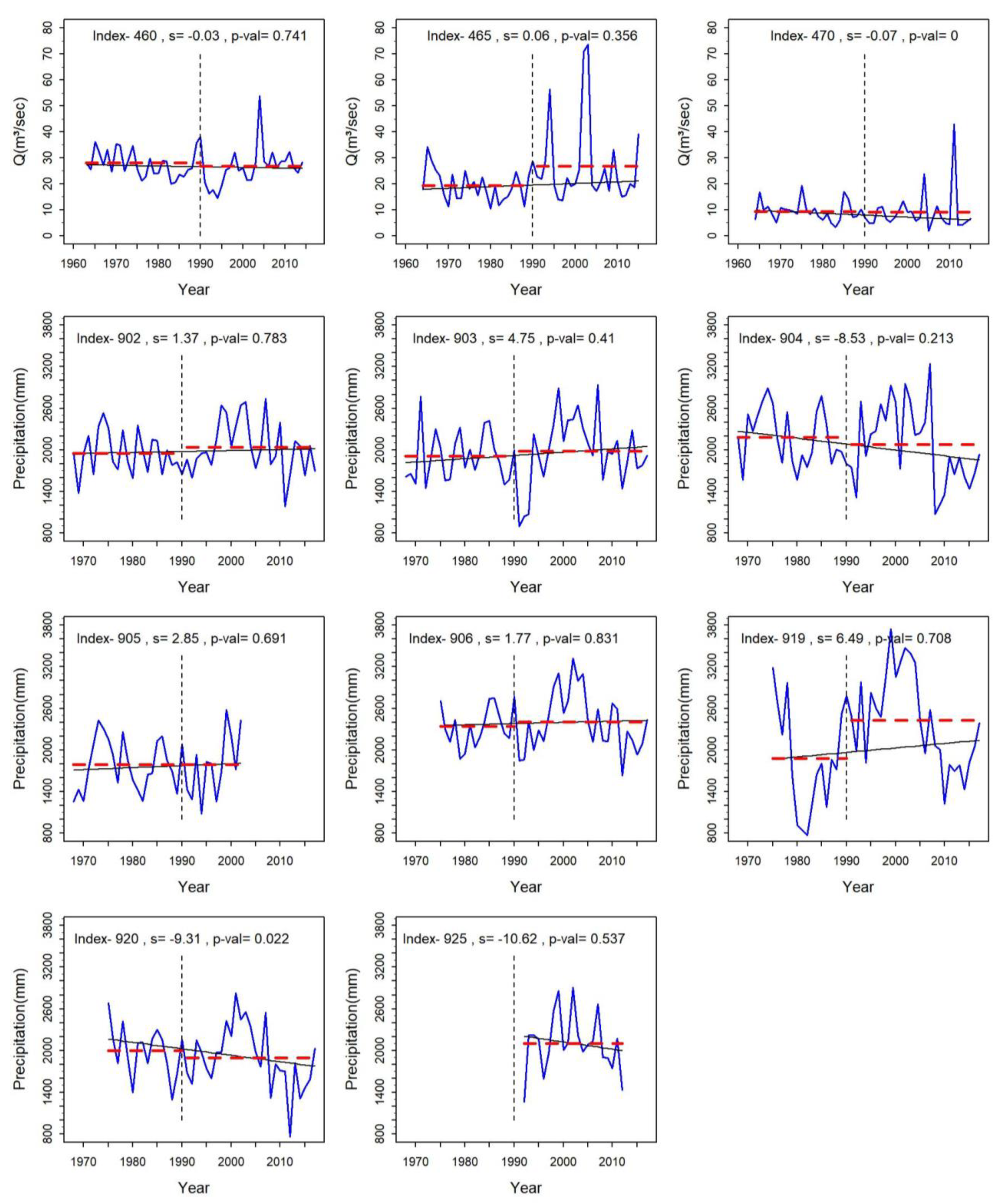
• There is a decreasing trend in streamflow observed at two hydrological stations post-1990. The rate of decrease at Manahari (station 465), a major tributary of the EER watershed, and Lothar Khola (station 470) for the period of 1991–2015 are 0.097 m³/s/yr and 0.054 m³/s, respectively. In the case of precipitation, most of the precipitation has statistically insignificant trends. For example, station 920, though there is a statistically significant decrease for the period of 1975–2017, there is a decreasing trend of 15 mm/year (insignificant) after 1990.
• Most of alterations/decrease in streamflow in the EER watershed after 1990 are attributed to the anthropogenic origin, though the rate of alteration varies across the stations. Climate-induced alterations in streamflow are associated dominantly to evapotranspiration.
• Streamflow alterations are having implications to water and food security; river health and aquatic biodiversity; and groundwater abstraction. However, a separate study is required to quantify precisely the extent of impacts.

To ensure water and food security, river health, aquatic biodiversity, and to be able sustainably abstract groundwater, it is recommended to devise strategies for water use efficiency through both supply-and demand-side management of water. It is also crucial to develop a water co-operation framework among the local governments, which share the same water resources, for strategic and sustainable use the water resources, and river health preservation.

References

1. Sharma, P.J.; Patel, P.L.; Jothiprakash, V. Impact of Rainfall Variability and Anthropogenic Activities on Streamflow Changes and Water Stress Conditions across Tapi Basin in India. Sci. Total Environ. 2019. [Google Scholar] [CrossRef] [PubMed]
2. Wester, P.; Mishra, A.; Mukherji, A.; Shrestha, A.B. The Hindu Kush Himalaya Assessment- Mountains, Climate Change, Sustainability and People; Wester, P., Mishra, A., Mukherji, A., Shrestha, A.B., Eds.; Springer Nature Switzerland AG: Basel, Switzerland, 2019. [Google Scholar] [CrossRef] [Green Version]
3. Ahn, K.H.; Merwade, V. Quantifying the Relative Impact of Climate and Human Activities on Streamflow. J. Hydrol. 2014. [Google Scholar] [CrossRef]
4. Buendia, C.; Batalla, R.J.; Sabater, S.; Palau, A.; Marcé, R. Runoff Trends Driven by Climate and Afforestation in a Pyrenean Basin. Land Degrad. Dev. 2016. [Google Scholar] [CrossRef] [Green Version]
5. Mallakpour, I.; Villarini, G. A Simulation Study to Examine the Sensitivity of the Pettitt Test to Detect Abrupt Changes in Mean. Hydrol. Sci. J. 2016. [Google Scholar] [CrossRef] [Green Version]
6. Beaulieu, C.; Chen, J.; Sarmiento, J.L. Change-Point Analysis as a Tool to Detect Abrupt Climate Variations. Philos. Trans. R. Soc. A Math. Phys. Eng. Sci. 2012. [Google Scholar] [CrossRef] [PubMed] [Green Version]
7. Zhu, Y.; Wang, W.; Liu, Y.; Wang, H. Runoff Changes and Their Potential Links with Climate Variability and Anthropogenic Activities: A Case Study in the Upper Huaihe River Basin, China. Hydrol. Res. 2015. [Google Scholar] [CrossRef]
8. Nune, R.; George, B.A.; Teluguntla, P.; Western, A.W. Relating Trends in Streamflow to Anthropogenic Influences: A Case Study of Himayat Sagar Catchment, India. Water Resour. Manag. 2014. [Google Scholar] [CrossRef] [Green Version]
9. Abeysingha, N.S.; Singh, M.; Sehgal, V.K.; Khanna, M.; Pathak, H. Analysis of Trends in Streamflow and its Linkages with Rainfall and Anthropogenic Factors in Gomti River Basin of North India | SpringerLink. Available online: https://link.springer.com/article/10.1007/s00704-015-1390-5 (accessed on 1 March 2020).
10. Somorowska, U.; Łaszewski, M. Quantifying Streamflow Response to Climate Variability, Wastewater Inflow, and Sprawling Urbanization in a Heavily Modified River Basin. Sci. Total Environ. 2019. [Google Scholar] [CrossRef]
11. Salmoral, G.; Willaarts, B.A.; Troch, P.A.; Garrido, A. Drivers Influencing Streamflow Changes in the Upper Turia Basin, Spain. Sci. Total Environ. 2015. [Google Scholar] [CrossRef]
12. Li, B.; Li, C.; Liu, J.; Zhang, Q.; Duan, L. Decreased Streamflow in the Yellow River Basin, China: Climate Change or Human-Induced? Water 2017, 9, 116. [Google Scholar] [CrossRef]
13. Pettitt, A.N. A Non-Parametric Approach to the Change-Point Problem. Appl. Stat. 1979. [Google Scholar] [CrossRef]
14. Alexandersson, H.; Moberg, A. Homogenization of Swedish Temperature Data. Part I: Homogenity Test for Linear Trends. Int. J. Climatol. 1997, 17, 25–34. [Google Scholar] [CrossRef]
15. Villarini, G.; Serinaldi, F.; Smith, J.A.; Krajewski, W.F. On the Stationarity of Annual Flood Peaks in the Continental United States during the 20th Century. Water Resour. Res. 2009. [Google Scholar] [CrossRef]
16. Liang, W.; Bai, D.; Wang, F.; Fu, B.; Yan, J.; Wang, S.; Yang, Y.; Long, D.; Feng, M. Quantifying the Impacts of Climate Change and Ecological Restoration on Streamflow Changes Based on a Budyko Hydrological Model in China’s Loess Plateau. Water Resour. Res. 2015. [Google Scholar] [CrossRef]
17. Hamed, K.H.; Ramachandra Rao, A. A Modified Mann-Kendall Trend Test for Autocorrelated Data. J. Hydrol. 1998. [Google Scholar] [CrossRef]
18. Kahya, E.; Kalayci, S. Trend Analysis of Streamflow in Turkey. J. Hydrol. 2004. [Google Scholar] [CrossRef]
19. Gautam, M.R.; Acharya, K. Streamflow Trends in Nepal. Hydrol. Sci. J. 2012. [Google Scholar] [CrossRef]
20. Zheng, H.; Zhang, L.; Zhu, R.; Liu, C.; Sato, Y.; Fukushima, Y. Responses of Streamflow to Climate and Land Surface Change in the Headwaters of the Yellow River Basin. Water Resour. Res. 2009. [Google Scholar] [CrossRef]
21. Gao, P.; Mu, X.M.; Wang, F.; Li, R. Changes in Streamflow and Sediment Discharge and the Response to Human Activities in the Middle Reaches of the Yellow River. Hydrol. Earth Syst. Sci. 2011. [Google Scholar] [CrossRef] [Green Version]
22. Wu, J.; Miao, C.; Zhang, X.; Yang, T.; Duan, Q. Detecting the Quantitative Hydrological Response to Changes in Climate and Human Activities. Sci. Total Environ. 2017. [Google Scholar] [CrossRef]
23. Jiang, S.; Ren, L.; Yong, B.; Fu, C.; Yang, X. Analyzing the Effects of Climate Variability and Human Activities on Runoff from the Laohahe Basin in Northern China. Hydrol. Res. 2012. [Google Scholar] [CrossRef]
24. ICIMOD. Nepal Land Cover. Available online: http://geoapps.icimod.org/landcover/nepallandcover/ (accessed on 2 March 2020).
25. Moritz, S.; Bartz-Beielstein, T. ImputeTS: Time Series Missing Value Imputation in R. R J. 2017. [Google Scholar] [CrossRef] [Green Version]
26. Zhang, Y.; Guan, D.; Jin, C.; Wang, A.; Wu, J.; Yuan, F. Analysis of Impacts of Climate Variability and Human Activity on Streamflow for a River Basin in Northeast China. J. Hydrol. 2011. [Google Scholar] [CrossRef]
27. Zhang, H.; Xu, W.; Xu, X.; Lu, B. Responses of Streamflow to Climate Change and Human Activities in a River Basin, Northeast China. Adv. Meteorol. 2017. [Google Scholar] [CrossRef]
28. Alexandersson, H. A Homogeneity Test Applied to Precipitation Data. J. Climatol. 1986, 6, 661–675. [Google Scholar] [CrossRef]
29. Pandžić, K.; Kobold, M.; Oskoruš, D.; Biondić, B.; Biondić, R.; Bonacci, O.; Likso, T.; Curić, O. Standard Normal Homogeneity Test as a Tool to Detect Change Points in Climate-Related River Discharge Variation: Case Study of the Kupa River Basin. Hydrol. Sci. J. 2020. [Google Scholar] [CrossRef]
30. Javari, M. Trend and Homogeneity Analysis of Precipitation in Iran. Climate 2016, 4, 44. [Google Scholar] [CrossRef]
31. Mann, H.B.; Whitney, D.R. On a Test of Whether One of Two Random Variables Is Stochastically Larger than the Other. Ann. Math. Stat. 1947. [Google Scholar] [CrossRef]
32. Beaver, R.J.; Lehmann, E.L. Nonparametrics: Statistical Methods Based on Ranks. Biometrics 1976. [Google Scholar] [CrossRef]
33. Hirsch, R.M.; Slack, J.R.; Smith, R.A. Techniques of Trend Analysis for Monthly Water Quality Data. Water Resour. Res. 1982. [Google Scholar] [CrossRef] [Green Version]
34. Pirnia, A.; Golshan, M.; Darabi, H.; Adamowski, J.; Rozbeh, S. Using the Mann-Kendall Test and Double Mass Curve Method to Explore Stream Flow Changes in Response to Climate and Human Activities. J. Water Clim. Chang. 2019. [Google Scholar] [CrossRef]
35. Zhang, Z.; Xu, C.Y.; El-Tahir, M.E.H.; Cao, J.; Singh, V.P. Spatial and Temporal Variation of Precipitation in Sudan and Their Possible Causes during 1948–2005. Stoch. Environ. Res. Risk Assess. 2012. [Google Scholar] [CrossRef] [Green Version]
36. Zhang, Q.; Liu, C.; Xu, C.Y.; Xu, Y.; Jiang, T. Observed Trends of Annual Maximum Water Level and Streamflow during Past 130 Years in the Yangtze River Basin, China. J. Hydrol. 2006. [Google Scholar] [CrossRef]
37. Partal, T.; Kahya, E. Trend Analysis in Turkish Precipitation Data. Hydrol. Process. 2006. [Google Scholar] [CrossRef]
38. Wagner, A.K.; Soumerai, S.B.; Zhang, F.; Ross-Degnan, D. Segmented Regression Analysis of Interrupted Time Series Studies in Medication Use Research. J. Clin. Pharm. Ther. 2002. [Google Scholar] [CrossRef] [PubMed]
39. Jaiswal, R.K.; Lohani, A.K.; Tiwari, H.L. Statistical Analysis for Change Detection and Trend Assessment in Climatological Parameters. Environ. Process. 2015. [Google Scholar] [CrossRef] [Green Version]
40. Zarenistanak, M.; Dhorde, A.G.; Kripalani, R.H. Trend Analysis and Change Point Detection of Annual and Seasonal Precipitation and Temperature Series over Southwest Iran. J. Earth Syst. Sci. 2014. [Google Scholar] [CrossRef]
41. Klein Tank, A.B.G.; Zwiers, F.W. Guidelines on analysis of extremes in a changing climate in support of informed decisions for adaptation. World Meteorol. Organ. 2009, 72, 55. [Google Scholar]
42. Sankarasubramanian, A.; Vogel, R.M.; Limbrunner, J.F. Climate Elasticity of Streamflow in the United States. Water Resour. Res. 2001. [Google Scholar] [CrossRef]
43. Schreiber, P. Über Die Beziehungen Zwischen Dem Niederschlag Und Der Wasserführung Der Flüsse in Mitteleuropa. Z. Meteorol 1904, 21, 441–452. [Google Scholar]
44. Ol’dekop, E.M. On Evaporation from the Surface of River Basins: Transactions on Meteorological Observations. Lur-Evskogo; University of Tartu: Tartu, Estonia, 1911. (In Russian) [Google Scholar]
45. Budyko, M.I. Evaporation under Natural Conditions; Israel Program for Scientific Translations; Office of Technical Services U.S. Dept. of Commerce Washington: Jerusalem, Israel, 1948. [Google Scholar]
46. Pike, J.G. The Estimation of Annual Run-off from Meteorological Data in a Tropical Climate. J. Hydrol. 1964. [Google Scholar] [CrossRef]
47. Turc, L. Le Bilan d’eau Des Sols. Relation Entre La Precipitation, l’evaporation et l’e’coulement. Ann. Agron 1954, 5, 491–569. [Google Scholar]
48. Fu, G.; Charles, S.P.; Chiew, F.H.S. A Two-Parameter Climate Elasticity of Streamflow Index to Assess Climate Change Effects on Annual Streamflow. Water Resour. Res. 2007. [Google Scholar] [CrossRef]
49. Zhang, L.; Dawes, W.R.; Walker, G.R. Response of Mean Annual Evapotranspiration to Vegetation Changes at Catchment Scale. Water Resour. Res. 2001. [Google Scholar] [CrossRef]
50. CBS. National Population and Housing Census 2011(National Report). Gov. Nepal, Natl. Plan. Comm. Secr. Cent. Bu reau Stat. 2012, 270. [Google Scholar]
51. MoEWRI. Irrigation Master Plan Preparation through Integrated River Basin Planning (Main Report); Ministry of Energy, Water Resources and Irrigation: Kathmandu, Nepal, 2019.
52. MoAD. Statistical Information on Nepalese Agriculture 2011/12; Ministry of Agriculture Development: Kathmandu, Nepal, 2012.
53. MoAD. Statistical Information on Nepalese Agriculture 2014/15; Ministry of Agriculture Development: Kathmandu, Nepal, 2015.
54. MoAD. Statistical Information on Nepalese Agriculture, Time Series Information 1999/2000-2011/2012; Ministry of Agriculture Development: Kathmandu, Nepal, 2013; p. 354.
55. MoAD. Statistical Information on Nepalese Agriculture 2013/2014; Ministry of Agriculture Development: Kathmandu, Nepal, 2014; Volume 2014, p. 212.
56. MoAD. Statistical Information on Nepalese Agriculture 2016/17; Ministry of Agriculture Development: Kathmandu, Nepal, 2017.
57. Lytle, D.A.; Poff, N.L.R. Adaptation to Natural Flow Regimes. Trends Ecol. Evol. 2004. [Google Scholar] [CrossRef]
58. DeFries, R.; Eshleman, K.N. Land-Use Change and Hydrologic Processes: A Major Focus for the Future. Hydrol. Process. 2004. [Google Scholar] [CrossRef]
59. Poff, N.L.; Zimmerman, J.K.H. Ecological Responses to Altered Flow Regimes: A Literature Review to Inform the Science and Management of Environmental Flows. Freshwater Biol. 2010. [Google Scholar] [CrossRef]
60. Gober, P.; Wheater, H.S. Socio-Hydrology and the Science–Policy Interface: A Case Study of the Saskatchewan River Basin. Hydrol. Earth Syst. Sci. 2014. [Google Scholar] [CrossRef] [Green Version]
61. Wei, J.; Wei, Y.; Western, A. Evolution of the Societal Value of Water Resources for Economic Development versus Environmental Sustainability in Australia from 1843 to 2011. Glob. Environ. Chang. 2017. [Google Scholar] [CrossRef]
62. Industrial District Management Limited. Aaudhogik Bikas Byawasthapan Limited Ko Smarika; Industrial District Management Limited: Kathmandu, Nepal, 2018. [Google Scholar]
63. IDM. Present State of Industrial Districts. Available online: https://idm.org.np/present-state-of-industrial-districts (accessed on 2 March 2020).
64. HSMC. City Profile of Hetauda Sub-Metropolitan City (HSMC); Office of the Municipal Executive: Hetauda, Nepal, 2017. [Google Scholar]
65. Pohlert, T. No Non-Parametric Trend Tests and Change-Point Detection. CC BY-ND 2018, 4, 18. [Google Scholar]
66. Mann, H.B. Nonparametric Tests Against Trend. Econometrica 1945. [Google Scholar] [CrossRef]
67. Kendall, M.G. Rank Correlation Methods, 4th ed.; The Griffin: London, UK, 1957. [Google Scholar]
68. Douglas, E.M.; Vogel, R.M.; Kroll, C.N. Trends in Floods and Low Flows in the United States: Impact of Spatial Correlation. J. Hydrol. 2000, 240, 90–105. [Google Scholar] [CrossRef]
69. Sneyers, R. On the Statistical Analysis of Series of Observations. World Meteorol. Organ. 1990. [Google Scholar] [CrossRef]
70. Sen, P.K. Estimates of the Regression Coefficient Based on Kendall’s Tau. J. Am. Stat. Assoc. 1968. [Google Scholar] [CrossRef]
71. Climate and life/by M. I. Budyko. English ed. Edited by David H. Miller.-Version details-Trove. Available online: https://trove.nla.gov.au/work/21788574?q&versionId=26211710 (accessed on 1 March 2020).
Figure 1. Location and topography of the Extended East Rapti (EER) watershed and associated administrative boundaries.
Sustainability 12 03829 g001
Figure 2. Land use/cover (LULC), river network, and location of hydro-meteorological stations in the Extended East Rapti (EER) watershed (Source: LULC data are based on ICIMOD [24]).
Sustainability 12 03829 g002
Figure 3. Population density (persons/km2) across 15 Palikas in the EER watershed.
Sustainability 12 03829 g003
Figure 4. The methodological framework used in this study. Q, streamflow; P, precipitation; SNH, standard normal homogeneity.
Sustainability 12 03829 g004
Figure 5. Flowchart with the methodology adopted in this study. ARIMA, autoregressive integrated moving average; IDW, inverse distance weighting; MMK, modified Mann-Kendal test, SR, spearman rho.
Sustainability 12 03829 g005
Figure 6. Trends in annual streamflow and precipitation time series in Extended East Rapti (EER) watershed. s, Sen’s slope, with positive and negative values representing increasing and decreasing trend, respectively. The red dashed line shows the mean values before and after 1990.
Sustainability 12 03829 g006