Abstract
Enhancing environmental sustainability in maritime shipping has emerged as an important topic for both firms in shipping-related industries and policy makers. Speed optimization has been proven to be one of the most effective operational measures to achieve this goal, as fuel consumption and greenhouse gas (GHG) emissions of a ship are very sensitive to its sailing speed. Existing research on ship speed optimization does not differentiate speed through water (STW) from speed over ground (SOG) when formulating the fuel consumption function and the sailing time function. Aiming to fill this research gap, we propose a speed optimization model for a fixed ship route to minimize the total fuel consumption over the whole voyage, in which the influence of ocean currents is taken into account. As the difference between STW and SOG is mainly due to ocean currents, the proposed model is capable of distinguishing STW from SOG. Thus, in the proposed model, the ship’s fuel consumption and sailing time can be determined with the correct speed. A case study on a real voyage for an oil products tanker shows that: (a) the average relative error between the estimated SOG and the measured SOG can be reduced from 4.75% to 1.36% across sailing segments, if the influence of ocean currents is taken into account, and (b) the proposed model can enable the selected oil products tanker to save 2.20% of bunker fuel and reduce 26.12 MT of CO2 emissions for a 280-h voyage. The proposed model can be used as a practical and robust decision support tool for voyage planners/managers to reduce the fuel consumption and GHG emissions of a ship.
1. Introduction
Maritime transport is essential to the world’s economy, as over 90% of the world’s trade is carried by sea [1]. In the past few years, enhancing environmental sustainability in maritime shipping has emerged as an important topic not only for firms in shipping-related industries, but also for policy makers [2,3]. This is mainly related to the greenhouse gas (GHG) emissions from maritime transport. Although shipping is considered an environment-friendly mode of transport, there are still considerable GHG emissions associated with shipping operations [4]. These emissions represent a significant part of the total global GHG emissions and become a non-negligible contributor to global warming [5]. According to the International Maritime Organization (IMO), in the period of 2007–2012, international shipping emitted 1016 million tonnes of CO2 per year on average, accounting for about 3.1% of global emissions; and this share could grow by 50–250% by 2050 depending on the international trade growth and energy developments [6]. Therefore, the carbon footprint of maritime transport must be reduced from the perspective of the sustainable development of the environment.
GHG emissions from ships are directly proportional to fuel burned. Thus, improving ship energy efficiency is one of the possible solutions to reduce emissions from ships without influencing the outputs [7]. Measures for improving ship energy efficiency are divided into two categories, namely design measures and operational measures. The former include hull form optimization, propeller configuration, utilization of lightweight materials, etc., which apply only to new building vessels and require large investment [8]. Shipping companies tend to take operational measures on existing ships that can provide significant saving potentials with relatively low investment compared to the design measures [9]. Among the operational measures recommended by the Ship Energy Efficiency Management Plan (SEEMP), such as speed optimization, weather routing, hull maintenance and trim optimization, speed optimization has been proven to be the most effective one [10,11]. A main reason is that the fuel consumption of a ship is very sensitive to its sailing speed: fuel consumption per time unit, also known as fuel consumption rate (FCR), is a non-linear (at least cubic) function of sailing speed [12,13]. In addition to having significant fuel savings, speed optimization is easy to implement and costs almost nothing. These advantages of speed optimization make it a preferred measure for shipping companies to reduce fuel consumption and GHG emissions.
Speed optimization exists at different stages of ship voyage management, including pre-fixture, fixture, at departure and post-voyage evaluation. Existing Operations Research/Management Science (OR/MS) studies address ship speed optimization mainly at the strategic or tactical level (i.e., the average speed over a service or leg) with simple forms of fuel consumption function (e.g., cubic functions or variants of the Admiralty coefficient) [14]. These OR/MS studies mainly serve the stages of pre-fixture and fixture. Unlike existing OR/MS studies, the concern of this paper is the at departure stage, in which the weather forecast for the upcoming voyage is available, and thus ship fuel consumption can be predicted with a more realistic model. On this basis, ship speed can be optimized at a finer level (e.g., per day). Usually, at the departure stage, the route over the target voyage has already been determined at a higher level (e.g., ship routing). Here, a voyage represents the journey from the departure from one port to the arrival at the next port [14]. For the voyage under consideration, there is an estimated time of arrival (ETA) at the voyage’s destination port, which is determined according to the cargo handling plan; and the sailing route over the voyage is usually divided into several segments based on certain criteria (e.g., distance, maritime regulations and sea conditions). Therefore, the speed optimization problem for a fixed ship route can be described as follows: determining the speed for each segment in the route so that the fuel consumption of the ship over the whole voyage is minimized while the ETA is guaranteed. In this problem, the ship can be considered as either a tramp ship or a liner ship [15].
To solve the above-mentioned speed optimization problem, two functions need to be determined: (a) the relationship between FCR and sailing speed (i.e., the fuel consumption function); and (b) the relationship between sailing time and sailing speed (i.e., the sailing time function). Once these two functions are determined and the sailing speed for each segment is allocated, the fuel consumption and sailing time over the whole voyage can be readily obtained. In the literature, the fuel consumption function is usually formulated in three different forms. Organized in ascending order of complexity, they are: (a) a non-linear function of sailing speed; (b) a non-linear function of both sailing speed and ship payload; and (c) a complex function of sailing speed, ship payload and other factors that may impact FCR, such as the prevailing weather conditions [16]. The sailing time function is uniformly presented in the literature as the sailing distance divided by the sailing speed. However, to the best of our knowledge, the existing research on ship speed optimization does not differentiate speed through water (STW) from speed over ground (SOG) when formulating the above two functions. It is known from basic principles of ship propulsion that STW should be used when estimating a ship’s FCR, while according to nautical knowledge, SOG should be employed when calculating a ship’s sailing time. Therefore, STW should not be confused with SOG in speed optimization models. Otherwise, incorrect calculations of fuel consumption and/or sailing time will be obtained.
The difference between STW and SOG is mainly due to ocean currents. Generally, favorable ocean currents can accelerate the ship, while opposed currents can retard the ship [17]. Therefore, if a ship encounters favorable currents, its SOG will be greater than its STW, while in the opposite case the ship’s SOG will be less than its STW. This implies that ocean currents have a significant influence on the actual sailing speed (i.e., the SOG) of a ship and thus cannot be neglected in speed optimization models.
The purpose of this paper is to propose a ship speed optimization model considering the influence of ocean currents. In contrast to existing ship speed optimization models, the proposed model is capable of distinguishing STW from SOG. On this basis, the ship’s fuel consumption and sailing time can be determined using the correct speed. In other words, calculations of fuel consumption and sailing time can be more accurate. This will effectively improve the reliability of the ship speed optimization model, as fuel consumption and sailing time are main components of the model. At the departure stage of a ship voyage management, the proposed model can be used as a practical and robust tool by decision makers (e.g., the ship owner or the charterer) to reduce the fuel consumption and GHG emissions of a ship.
The remainder of this paper is organized as follows. Section 2 reviews existing scientific studies on ship speed optimization. Section 3 gives a thorough description of the problem considered, including a mathematical formulation of the problem. Section 4 describes the solution method for solving the proposed model. Section 5 conducts a case study over a voyage of an oil products tanker. Discussions on the application of the proposed speed optimization model are presented in Section 6. Finally, some conclusions are drawn in Section 7.
2. Literature Review
In the past decade, a growing number of studies on ship speed optimization have been conducted to address the environmental impacts of cargo shipping. One of the early studies, Fagerholt et al. [18], proposes a speed optimization problem for a fixed ship route with the assumption that fuel consumption per time unit is a cubic function of the sailing speed within certain speed limits. The objective of this problem is to determine the speed for each leg in the route so that the total fuel consumption is minimized while the port time windows are satisfied. The authors discretize the arrival times and solve the problem by using the shortest path algorithm. Subsequently, the same problem is solved by Hvattum et al. [19] and Kim et al. [15] with exact solution algorithms. Zhang et al. [20] extend the work of Fagerholt et al. [18] and study the optimality properties. All these studies focus on the technical side of speed optimization based on the simplified assumption that the rate of fuel consumption is the same across all legs on the route. Later, He et al. [21] relax this assumption and suggest a consumption function model which is a general continuously differentiable and strictly convex function, but without a concrete form of variable impacts, causing varying costs per unit of distance traveled by the ship.
With its basic function forms, ship speed optimization is incorporated into other ship operation problems at tactical and strategic levels, in order to reveal the direct impact of speed on the transit time and service quality of shipping [21,36]. Typical problems addressed are ship routing and scheduling [22,23,24,25,26], fleet deployment [27,28], berth allocation [29,30], bunker fuel management [31,32,33,34] and maintenance scheduling [35]. Relevant studies are listed in Table 1. In general, this set of OR/MS studies considers market-related variables (e.g., fuel price, market spot rate, charter party contracts), but does not take the effect of weather and sea conditions on ship speed into account, because at the tactical level (deployment stage in liner shipping or the pre-fixture and fixture stages in tramp shipping), the weather forecast for the target voyage is not available.

Table 1.
Speed optimization in tactical and strategic ship operations.
In recent years, researchers in the field of OR/MS have begun to address ship speed optimization at the operational level, in order to capture the real-world scenarios more precisely. Apart from sailing speed and ship payload, weather and sea conditions, engine efficiency and other factors could also influence the ship’s fuel consumption rate. Hence, only by considering such factors can we provide operational-level decisions on ship speeds. Several of the recent studies treat the fuel consumption rate as a stochastic variable and employ a stochastic term to represent the influence of factors other than ship speed (or ship speed and ship payload). Sheng et al. [37] propose a multistage dynamic model that addresses speed determination and refueling decisions simultaneously, in which the stochastic nature of the fuel prices and the fuel consumption rate are taken into account. The stochastic term of the fuel consumption rate is assumed to follow a normal distribution, with a zero mean and a constant coefficient of variation under different ship speeds. Similarly, Zhen et al. [38] present a threshold-based policy for optimal ship refueling decisions, and the mean fuel consumption rate is assumed to follow the Truncated Normal Distribution. Their model can potentially be extended to evaluate several fuel bunkering policies. Considering this point, De et al. [39] develop a model that addresses a joint problem of speed optimization and bunker fuel management by considering slow steaming and taking into account different fuel bunkering policies, stochastic fuel consumption on each leg of the voyage and a stochastic fuel price at each port. However, operational-level studies modeling the fuel consumption rate as a stochastic factor are still too simple, for the fuel consumption rate is influenced by many factors (speed, draft, trim, weather and sea conditions, etc.) and it is nearly impossible to accurately describe the influence of those factors by using a probability distribution function.
To accurately estimate the fuel consumption for each leg at the operational level, a more interdisciplinary approach can be to use a deterministic fuel consumption model based on physical principles of ship propulsion or a machine-learning model involving most of the determinants of the fuel consumption rate. For example, Li et al. [40] work on a speed optimization problem for a given route between two ports, in which the influence of wind and irregular waves on ship sailing is taken into account. They develop a bi-objective optimization model to minimize fuel consumption and maximize operating cost reduction simultaneously. Li et al. [41] extend the work of Li et al. [40] by considering voluntary speed loss and GHG emissions. In order to address a ship sailing speed and trim optimization problem over a voyage, Du et al. [14] propose three viable countermeasures within an effective two-phase optimal solution framework. The optimization is based on two artificial neural network models that can quantify the synergetic influence of the sailing speed, displacement, trim, and weather and sea conditions on ship fuel consumption.
Based on the above literature review, we thus identified a research gap regarding speed optimization. Although several studies have addressed ship speed optimization at the operational level by using sophisticated fuel consumption functions to consider as many factors as possible, the influence of ocean currents on ship sailing has not had sufficient attention. Neglecting the influence of ocean currents on ship sailing will lead to the confusion of STW with SOG and result in incorrect calculations of fuel consumption and/or sailing time. This will eventually affect the accuracy of speed optimization models. The contribution of this paper is to address this gap by proposing a ship speed optimization model in which the comprehensive influence of still water resistance, wind, irregular waves and ocean currents on ship sailing is considered. In particular, this paper provides a method to involve the influence of ocean currents on ship sailing in speed optimization.
3. Problem Description and Mathematical Formulation
3.1. Problem Description
As mentioned in Section 1, this paper focuses on a speed optimization problem for a fixed ship route between two ports. This problem usually exists at the departure stage of ship voyage management. The research object of this problem is a single ship (either a tramp ship or a liner ship) whose main dimensions are known. The ship is loaded with a certain amount of cargo and will sail from the departure port A to the destination port B to perform a transportation mission. The ship payload is fixed during the voyage. Compared with the ship’s displacement, the amount of fuel consumed during the voyage is very small. Therefore, the ship’s displacement is assumed to be constant during the voyage. The ship departure time from port A is 0, and the ship arrival time at port B should not be later than the ETA at port B. The sailing route between port A and port B has already been determined at a higher level (e.g., ship routing). Weather and sea conditions (e.g., wind, waves and ocean currents) on this route have a significant influence on ship sailing. These meteorological data can be obtained via a real-time weather forecast. Based on them, we can group similar sea areas into the same sailing leg and divide the whole route into several segments. In each segment, we assume that: (a) the ship sails in a fixed heading; (b) weather and sea conditions can be viewed as identical; and (c) the ship travels using a constant brake power. These segments are connected by consecutive waypoints (incl. port A and port B) whose geographical coordinates (latitude and longitude) are known, and it can be known from assumption (a) that in each segment the ship will sail along the rhumb line. Based on this information, the distance (i.e., the rhumb line length) and course angle of each segment between two adjacent waypoints along the sailing route can be readily obtained (Ship course should be distinguished from ship heading. In navigation, the course of a ship is the cardinal direction in which the ship is to be steered, while the heading of a ship is the compass direction in which the ship’s bow is pointed [42]. The ship’s heading angle is the angle over water, while the ship’s course angle is the over-ground angle [43]).
During the voyage, the crew can set a speed for the ship by operating the main engine control system. This speed is the expected speed that the ship can reach under ideal weather and sea conditions (no wind, no waves, no ocean currents, etc.) and is usually referred to as the still water speed (SWS). In this paper, we take the SWS in each segment as the decision variable. As the ship’s main dimensions and payload are known, the brake power and FCR of the ship can be obtained from the fuel consumption function once the ship’s SWS is determined (please refer to Section 3.2.1). In practical scenarios, when the ship is sailing at this brake power, its STW is usually less than the set SWS due to the existence of wind and waves. The difference between the two is the involuntary speed loss. Additionally, due to the existence of ocean currents, the above STW is not equal to the ship’s SOG, which should be used to calculate the sailing time. Therefore, we should further consider the influence of ocean currents to determine the SOG (please refer to Section 3.2.2). For a specific segment, once the SOG is determined, the ship’s sailing time in this segment can be readily obtained.
Based on the obtained FCR and sailing time in each segment, main elements of the speed optimization model can be obtained, incl. the fuel consumption in each segment, the total fuel consumption over the whole voyage and the total sailing time over the whole voyage. The purpose of the speed optimization model is to determine the SWS for each segment with the objective of minimizing the total fuel consumption over the whole voyage. In addition to the ETA constraint, there are two further constraints that need to be satisfied. First, the SWS is constrained to change from its minimum to maximum values. Second, for the purpose of safety, the ship has a critical STW (maximum allowed STW) when sailing in wind and waves. Details of the speed optimization model can be seen in Section 3.2.3. The modeling steps of the speed optimization problem are illustrated in Figure 1.
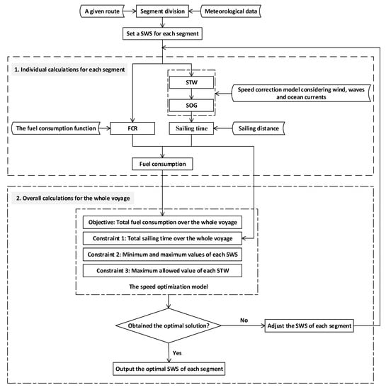
Figure 1.
Modeling steps of the speed optimization problem.
3.2. Mathematical Formulation
3.2.1. The Fuel Consumption Function
The DTU-SDU method is used to estimate the brake power and FCR of the ship. This method is developed by Kristensen and Lützen, and is applicable to three major ship types: container ships, bulk carriers and tankers [44]. According to the method, when a ship is sailing in still water, its total resistance can be determined by the following equation:
where is the mass density of seawater in metric tons per m3 (MT/m3), is the wetted surface of the hull in m2, is the ship’s SWS in m/s and is the total resistance coefficient.
The total resistance coefficient consists of four components:
where is the frictional resistance coefficient, is the incremental resistance coefficient, is the air resistance coefficient and is the residual resistance coefficient.
Once the ship’s total resistance is determined, the effective power of the ship, , can be obtained according to the following equation:
Then, the required brake power of the ship, , can be determined from according to the following equations:
where is the total efficiency from to , is the hull efficiency, is the propeller open water efficiency, is the relative rotative efficiency and is the shaft efficiency.
Finally, the ship’s FCR, (MT/h), can be determined as follows:
where is the Specific Fuel Oil Consumption (SFOC) of the ship’s main engine in g/kWh, which varies with the main engine load and can be obtained from the main engine performance documents.
Once the ship’s main dimensions, payload and SWS are known, the values of , , , , , , , and can be calculated based on empirical formulae developed by Kristensen and Lützen [44]. Therefore, for a given ship carrying a certain amount of cargo, we can estimate the FCR of the ship at various SWSs according to Equations (1)–(6).
3.2.2. The Speed Correction Model
To define the sailing time function, we need first to estimate the involuntary speed loss due to added resistance in wind and waves under the assumption that the ship’s brake power remains constant. An approximate method developed by Kwon [45] can be used to achieve this goal. Kwon’s method is easy and practical to use, as it depends on only a few parameters. Meanwhile, this method shows good accuracy in comparison to more extensive calculation methods [45]. According to Kwon [45], the percentage of speed loss can be expressed as:
from which, by using the relationship , it follows that the ship speed in the selected weather (wind and irregular waves) conditions may be expressed as:
where:
- : The ship’s STW in the selected weather (wind and irregular waves) conditions, given in m/s;
- : Absolute speed loss, given in m/s;
- : Direction reduction coefficient, which is a non-dimensional number, dependent on the weather direction angle (with respect to the ship’s bow) and the Beaufort number , as shown in Figure 2 and Table 2;
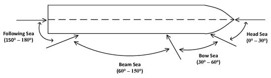 Figure 2. Weather direction.
Table 2. Direction reduction coefficient .
Figure 2. Weather direction.
Table 2. Direction reduction coefficient . - : Speed reduction coefficient, which is a non-dimensional number, dependent on the ship’s block coefficient, , the loading conditions and the Froude number, , as shown in Table 3;
Table 3. Speed reduction coefficient .
- : Ship form coefficient, which is a non-dimensional number, dependent on the ship type, the Beaufort number, , and the ship displacement, , in m3, as shown in Table 4.
Table 4. Ship form coefficient .
The weather direction angle (with respect to the ship’s bow) can be calculated according to the following logical statement [46]:
where is the wind direction angle (with respect to the True North) and is the ship heading angle (with respect to the True North). Here, the wave direction angle is assumed to be the same as the wind direction angle, which is true in most instances of surface waves [47].
The Beaufort number, , is an empirical measure that relates wind speed to observed conditions at sea or on land. It is defined by a range of wind speeds at the standard height. Please refer to Townsin et al. [48] and Yang et al. [9] for more details.
The Froude number, , can be determined by the following equation:
where is the ship length between perpendiculars in m and is the acceleration of gravity in m/s2.
The ship’s block coefficient, , and displacement, , are associated with the ship’s main dimensions and payload, . Detailed formulae for calculating and can be seen in MAN Diesel & Turbo [49].
As can be seen from the above formulae and tables, for a given ship with a SWS , its corresponding STW in selected weather (wind and irregular waves) conditions can be readily estimated once the following parameters are available: ship type; ship’s main dimensions; ship’s loading conditions; ship payload, ; ship heading angle, ; wind direction angle, ; and Beaufort number, .
For the purpose of safety, the ship has a critical STW (maximum allowed STW) when sailing in wind and waves. When is greater than the critical STW, the ship must be slowed down, which is known as the voluntary speed reduction. In this paper, the following equations are used to calculate the critical STW [50,51]:
where is the critical STW in knots, is the significant wave height in m and is the weather direction angle (with respect to the ship’s bow) in radian.
To define the sailing time function more accurately, we need to correct the STW to the SOG by considering the influence of ocean currents. Actually, ocean currents can affect both the SOG and the ship course. Let denote the expected ship course angle (with respect to the True North), which can be obtained based on the geographical coordinates of two adjacent waypoints along the sailing route, as explained in Section 3.1. During the voyage, the ship heading angle, , is a manipulated parameter. If is set equal to , the ship will sail in an actual course of with an actual speed of due to the existence of ocean currents, as shown in Figure 3a. Therefore, in practice, the crew needs to choose a ship heading angle which is different from the expected ship course angle to correct the yaw caused by ocean currents and guarantee that the ship can sail in the expected course, as shown in Figure 3b. In Figure 3, is the current speed, given in m/s; is the current direction angle (with respect to the True North); and is the actual sailing speed, namely the SOG, given in m/s.
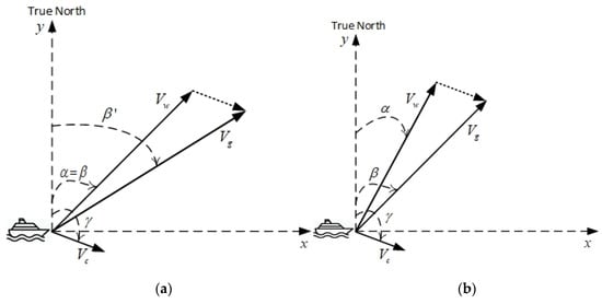
Figure 3.
Variations in speed and course due to ocean currents: (a) is set equal to and (b) is set different from to guarantee that the ship can sail in the expected course.
With the assistance of Figure 3b, we can develop formulae for calculating the SOG readily. According to the method of vector decomposition, the components of in the direction and the direction are and , respectively. Similarly, the components of in the direction and the direction are and , respectively. Therefore, the components of in the direction and the direction can be expressed as Equations (14) and (15), respectively:
Hence, according to the method of vector synthesis, the SOG can be determined by the following equation:
And the relationship among , and can be expressed as follows:
As can be seen from Equations (14)–(17), to calculate the SOG , we need first to determine the STW and the ship heading angle . As is also dependent on , determining the value of becomes the prerequisite for calculating . To address this problem, we present a heuristic algorithm, as shown in Section 4.1.
3.2.3. The Speed Optimization Model
In this section, a speed optimization model is developed for a fixed ship route between two ports to determine the SWS for each segment in the route, so that the fuel consumption of the ship over the whole voyage is minimized while the ETA is guaranteed. The notations of the speed optimization model are shown in Table 5.
Table 5.
Notations of the speed optimization model.
Based on the notations in Table 5, the speed optimization model can be formulated as follows:
subject to
The objective function (18) minimizes the ship fuel consumption over the whole voyage. Constraint (19) ensures that the ship arrival time at the destination port is no later than the ETA. Constraints (20) ensure that the set SWS in each segment is within the ship’s feasible SWS interval. Constraint (21) guarantees that the ship’s STW does not exceed the critical STW in wind and waves.
4. Solution Approach
It is challenging to use derivative-based methods to solve the speed optimization model presented in Section 3.2.3, since there is a very complicated relationship between the decision variable (i.e., ) and each of the derived variables (i.e., , and ). Hence, in this paper, a direct search method, namely a genetic algorithm (GA), is used for optimization. Before describing the GA in Section 4.2, a heuristic algorithm for determining the ship heading angle is presented in Section 4.1.
4.1. A Heuristic Algorithm for Determining the Ship Heading Angle
In this paper, as explained in Section 3.2.2, determining the ship heading angle, , is the prerequisite for ship speed optimization and needs to be addressed first. In order to address this problem, we present a heuristic algorithm, as shown in Algorithm 1.
| Algorithm 1. A heuristic algorithm for determining the ship heading angle. | |
| Input: | Ship type, ship’s main dimensions, ship’s loading conditions, , , , , , and . |
| Output: | and . |
| Basis: | Normally, . Hence, the difference between and will not be too great. |
| Step 1. | Replace in Equation (9) with to obtain the relative angle between and . This relative angle is denoted as . |
| Step 2. | Replace in Table 2 with to determine the weather direction. This weather direction is denoted as . |
| Step 3. | Assume that also belongs to , as the difference between and is small. |
| Step 4. | Calculate the value of according to the equations and tables in Section 3.2.2. In this step, the above is used as the weather direction. |
| Step 5. | Once the value of is determined, we can calculate the value of according to Equations (14), (15) and (17). |
| Step 6. | Calculate the value of based on the obtained (refer to Equation (9)). |
| Step 7. | Determine the weather direction to which belongs. This weather direction is denoted as . |
| Step 8. | If equals to , output the obtained in Step 4 and the obtained in Step 5; Otherwise, re-execute Step 4 and Step 5 using and output the obtained and . |
As can be seen from Algorithm 1, the proposed heuristic algorithm can be used to determine the values of and simultaneously. Once and are determined, the SOG can be readily calculated according to Equations (14)–(16).
4.2. The GA for Speed Optimization
A real-coded GA is employed to solve the speed optimization problem. The procedures of the GA are descripted as follows:
- Step 1:
- Population initialization. For a sailing route with segments, the individual is represented as a vector of length . The following equation represents the th individual of the population:Then, a population of individuals is represented as a matrix:Each individual of the population represents a solution to the speed optimization. is the in th segment of the th solution.The first step of the GA is to initialize the . To this end, the genes of each chromosome (individual) are randomly generated within the range of and .
- Step 2:
- Fitness evaluation. Evaluating the fitness value of each individual according to the following equation:where is the FCR corresponding to , is the SOG corresponding to , is the penalty function that is related to Constraint (19) and is the penalty function that is related to Constraint (21).The penalty functions and are defined as follows:where is a large enough number, is the STW corresponding to and is the critical STW in segment .
- Step 3:
- Selection. Selecting parent individuals to build a mating pool. The selection strategy used in this paper is the roulette wheel.
- Step 4:
- Reproduction. Repeat times:
- (a)
- Crossover. Picking up two parent individuals randomly from the mating pool and creating offspring by using a crossover operator. The crossover operator used in this paper is the BLX-α [52]. The crossover probability is .
- (b)
- Mutation. The above newly generated offspring are reprocessed with a mutation operator. The mutation operator used in this paper is the uniform random mutation. The mutation probability is .
- (c)
- Adding the children individuals to a new population.
- Step 5:
- Termination. Stopping the GA when it has reached a predefined number of generations .
5. Case Study
In this section, a voyage of an oil products tanker is selected to perform the case study. The main dimensions of the selected ship are shown in Table 6, the SFOC curve of the ship’s main engine is shown in Figure 4, and the voyage plan is shown in Table 7.
Table 6.
Main dimensions of the selected ship.
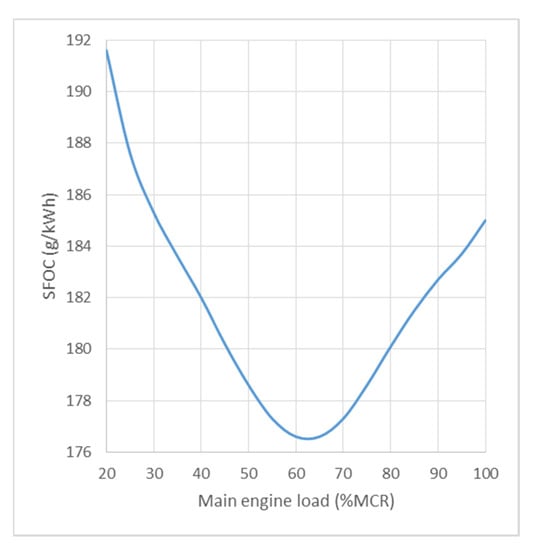
Figure 4.
The SFOC curve of the ship’s main engine.
Table 7.
Voyage plan.
The sailing route between port A and port B is divided into 12 segments according to the weather and sea conditions on this route. These segments are connected by 13 consecutive waypoints (incl. port A and port B). The information of these waypoints and segments is presented in Table 8. Parts of these data are obtained directly from the ship’s noon reports, and others are calculated from the available data. In Table 8, please note that (a) waypoint 1 represents port A and waypoint 13 represents port B; and (b) a segment is defined as the route between the current waypoint and the previous waypoint, e.g., segment 3 is the sailing route from waypoint 3 to waypoint 4.
Table 8.
Information of waypoints and segments of the selected route.
5.1. Model Verification
The reliability of the speed optimization model depends mainly on two factors: (a) the accuracy of the fuel consumption function in Section 3.2.1 and (b) the accuracy of the speed correction model in Section 3.2.2. Therefore, before optimizing the ship’s speed, we validate the above two models based on the measured data.
5.1.1. Verification of the Fuel Consumption Function
For segment , the FCR can be estimated using the fuel consumption function in Section 3.2.1 and the value of in Table 8. Then, we can estimate the fuel consumption in segment by multiplying by the corresponding sailing time in Table 8. For each segment, the measured and the estimated fuel consumption are compared. Meanwhile, the relative error between them is calculated, as shown in Table 9. The following two figures can be extracted from Table 9: (a) among the 12 segments of the target route, the maximum relative error is less than 6.50%; and (b) from an overall perspective, the average relative error of these 12 segments is 3.75%. These figures indicate that the fuel consumption function we proposed in Section 3.2.1 has a high accuracy. Intuitive verification results of the fuel consumption function are shown in Figure 5.
Table 9.
Verification results of the fuel consumption function.
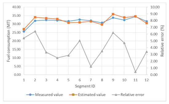
Figure 5.
Intuitive verification results of the fuel consumption function.
5.1.2. Verification of the Speed Correction Model
For segment , the measured value of can be calculated based on and the corresponding sailing time in Table 8. Meanwhile, the estimated value of can be obtained based on the value of in Table 8 and the speed correction model in Section 3.2.2. Here, two estimated values of are obtained. The first one is obtained under the condition that the influence of ocean currents is not considered, while the second one is calculated under the condition that the influence of ocean currents is taken into account. In the first case, the estimated value of is actually the estimated value of . For each segment, the measured and the estimated are compared, and the relative error between them is calculated, as shown in Table 10. From this table, we can see that: (a) when the influence of ocean currents is not considered, the average relative error of the speed correction model is 4.75%; and (b) when the influence of ocean currents is taken into account, this value becomes 1.36%. Intuitive verification results of the speed correction model are shown in Figure 6 and Figure 7. Based on these results, we can draw the conclusion that the error between the estimated and the measured can be effectively reduced if the influence of ocean currents is taken into account.
Table 10.
Verification results of the speed correction model.
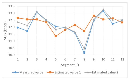
Figure 6.
Comparison of measured speed over ground (SOG) and estimated SOG.
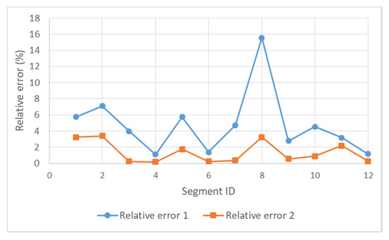
Figure 7.
Comparison of relative error 1 and relative error 2.
5.2. Speed Optimization Results and Analyses
The solution approach in Section 4 is programmed with R programming language. The parameter settings of the GA are presented in Table 11. We ran the program 10 times. The average running time of the program was 14.86 s. The results of the 10 runs of the program were consistent, indicating that the algorithm had a good stability. We randomly selected one of the above 10 running results for further analysis. The convergence curve of this run is presented in Figure 8. Based on this figure, we can draw the conclusion that the designed GA has good convergence and convergence speed on the target problem.
Table 11.
The parameter settings of the genetic algorithm (GA).
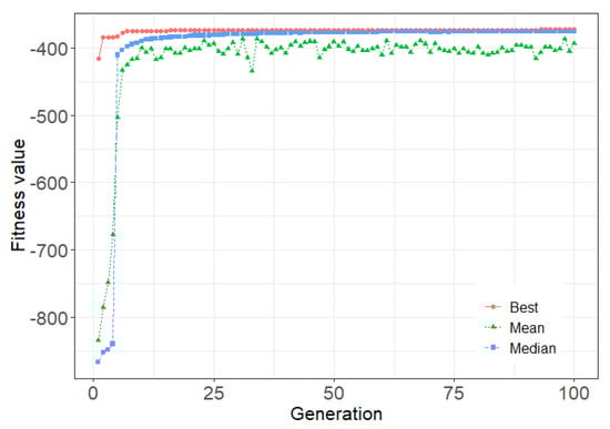
Figure 8.
Convergence curve of the GA.
After optimization, the SWS, SOG, sailing time, FCR and fuel consumption of each segment are shown in Table 12. From this table, we can see that: (a) the total sailing time over the whole voyage is 280.00 h, which remains unchanged; and (b) the total fuel consumption over the whole voyage is 372.62 MT, which is 8.38 MT less than the actual value (i.e., 381.00 MT). Considering that there is a little deviation between the actual and the estimated fuel consumption, the latter should be chosen as the benchmark for comparison. Before optimization, the estimated total fuel consumption over the whole voyage is 381.01 MT. Therefore, after optimization, the total fuel consumption over the whole voyage is actually reduced by 8.39 MT, accounting for 2.20% of the estimated fuel consumption before optimization. We can thus conclude that the proposed speed optimization model can help the selected oil products tanker save about 2.20% of bunker fuel to complete a 280-h voyage. The SWS, SOG, sailing time and fuel consumption of each segment before and after optimization are compared in Figure 9.
Table 12.
Results of ship speed optimization.
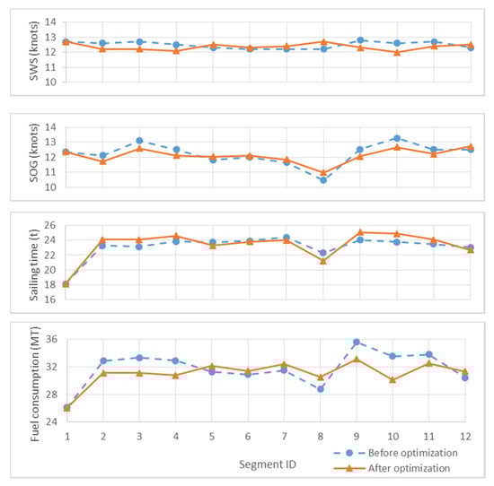
Figure 9.
Comparison of still water speed (SWS), SOG, sailing time and fuel consumption of each segment before and after optimization.
5.3. Analysis of GHG Emissions
The impact of the speed optimization model on GHG emissions from ships is also a major concern of this paper. According to the IMO [6], CO2 is the dominant GHG produced by shipping. Hence, we mainly emphasize emissions of CO2 in our analysis. As mentioned in Section 1, GHGs emitted by ships are directly proportional to the fuel they burn. In that sense, the CO2 emissions from ships can be estimated as follows:
The CO2 emission factor is related to the fuel type. The selected oil products tanker mainly consumes heavy fuel oil (HFO), whose CO2 emission factor is 3.114 MT/MT of fuel, according to the IMO [6]. For the target voyage, the reduction of CO2 emissions due to speed optimization can be calculated readily by multiplying the above CO2 emission factor by the fuel saving of 8.39 MT. Specifically, after optimization, the reduction of CO2 emissions over a 280-h voyage is 26.12 MT. The amount of CO2 emissions over the target voyage is shown in Figure 10.
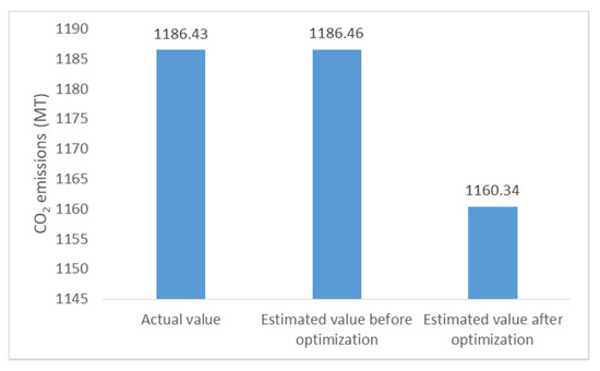
Figure 10.
The amount of CO2 emissions over the target voyage.
An aspect for further clarification is that many vessels have auxiliary engines for power production running on various fuels (e.g., diesel). This paper only includes an estimate of main engine and not on auxiliary engine GHG emissions.
6. Discussions of Model Application and Study Results
In shipping practice, speed optimization can be performed at different stages of ship voyage management, including pre-fixture, fixture, at departure and post voyage evaluation. At pre-fixture and fixture stages, fuel buyers (i.e., the ship owner if the ship is on spot charter, or the charterer if the ship is on time or bareboat charter) will often set the ship’s speed to optimize market-related variables and meet obligations of charter party contracts [16]. The so-called market-related variables mainly refer to fuel prices and market spot rates. As demonstrated by Psaraftis and Kontovas [53], the non-dimensional ratio of the fuel price divided by the spot rate is a key indicator of the need for speed optimization. Specifically, a lower ratio (fuel price/spot rate) will lead to recommendation of a high optimal speed for the ship, assuming that the speed is not fixed by the charter party contract [16]. If an instructed ship speed is part of a charter party contract, the ship owner or the charterer will attempt to adhere to the set agreement. As the weather forecast for the target voyage is not available at these two stages, when optimizing speed the ship owner or the charterer can only estimate fuel costs with a very simple form of fuel consumption function (e.g., a cubic function of ship speed). Most of the existing ship speed optimization models in OR/MS literature mainly serve these two stages.
Unlike existing ship speed optimization models in OR/MS literature, the proposed model can be used at departure stage of ship voyage management. At this stage, the ratio of the fuel price divided by the spot rate is no longer a key determinant of the ship’s speed, as it will be a fixed value. In order to minimize the total fuel consumption, the ship owner or the charterer usually optimizes the ship’s speed at a more granular level (e.g., per day) based on the forecasted weather and sea conditions on the target route, and also preferably based on ocean currents.
Of course, the proposed speed optimization model is also applicable at the stage of post-voyage evaluation. The voyage is now accomplished, and the real weather and sea conditions of the sailing route is known. Based on the real weather and sea conditions, the ship owner or charterer can apply the proposed model to post-evaluate the voyage plan and explore the possibility of improving it for an upcoming assignment.
As part of our development of a speed optimization model, we made some assumptions in Section 3.1. Assumption (b) is that weather and sea conditions can be perceived as identical within a segment, and assumption (c) is that the ship travels using a constant brake power during each segment. Implication of this is that the SWS, STW and SOG all are constant during each segment/leg on the journey. In the case study, the sailing route was divided into 12 segments based on the ship’s noon reports, which are typically compiled every 24 h at noon resulting in a constant speed across 24 h of sailing time. This does not match the practical sailing situation, and it may be one of the reasons why the proposed speed optimization model can only help the selected oil products tanker save 2.20% of bunker fuel. In practical applications, the proposed model can be refined by using the actual weather forecast data. Weather forecast data usually have a spatial resolution (a certain degree of arc length) at either: 0.25°, 0.5°, 1.0° and 2.0°. For example, the 0.5° resolution represents an arc length of 30 nmi. Additionally, this data category also has a temporal resolution (the weather forecast update interval) at 3 h or 6 h. It should thus be possible for us to include weather forecast data with a spatial resolution of 0.5° and a temporal resolution of 6 h in future studies. Also, it should equivalently be possible for us to capture a ship’s brake power and other relevant navigational and engine room data every 6 h rather than every 24 h. By this means, the set speed of the ship can be adjusted every 6 h, and the actual sailing speed of the ship will change as the weather and sea conditions on the route change.
7. Conclusions
In this paper, we propose a speed optimization model for a fixed ship route to minimize the total fuel consumption over the whole voyage, in which the influence of ocean currents on ship sailing is taken into account. In contrast to existing speed optimization models, the proposed model is capable of distinguishing STW from SOG. On this basis, we can determine the ship’s fuel consumption and sailing time more accurately, by using the correct speed. This effectively improves the reliability of the speed optimization model, as fuel consumption and sailing time are main components of the model.
A case study was performed on a real voyage of an oil products tanker. Two important conclusions can be drawn from the computational results. First, the average relative error between the estimated SOG and the measured SOG for the 12 sailing segments can be reduced from 4.75% to 1.36% if the influence of ocean currents is taken into account, indicating that ocean currents have a significant influence on the actual sailing speed (i.e., the SOG) of a ship and thus cannot be neglected in the speed optimization models for the departure stage. Second, the proposed speed optimization model can potentially enable the selected oil products tanker to save app. 2.20% of bunker fuel consumption on a 280-h voyage, which also leads to a visible GHG emissions reduction.
The study’s main academic contribution is that it has investigated the theoretical and practical implications of including ocean currents into speed optimization models. From an industry practitioners’ perspective, this study provides a ship speed optimization model which potentially can be applied at departure stage of ship voyages by decision makers (e.g., the ship owner or the charterer) with the aim of reducing fuel consumption and GHG emissions of a ship. The study thus makes a small effort to support the maritime industry in meeting the 2030 and 2050 targets set for emissions by IMO.
The proposed speed optimization model has only been applied and tested on data from a single voyage of an oil products tanker, which obviously limits the robustness and generalizability of the study findings. We therefore call for further research to test and perhaps adjust the models developed based on a larger sample of vessels and voyages, perhaps even across different ship segments. An interesting direction for future research can potentially be to develop a two-stage speed optimization model by combining our proposed model with existing speed optimization models in the OR/MS literature. Specifically, at the first stage, the average speed over the target voyage can be determined based on market-related variables (e.g., fuel price and market spot rate) and charter party contracts. Then, at the second stage, the proposed model can be used to provide a solution to the daily speed planning of the ship based on the average speed obtained at the first stage.
Author Contributions
Conceptualization, L.Y. and G.C.; methodology, L.Y. and G.C.; investigation, L.Y. and G.C.; data curation, L.Y.; validation, L.Y.; writing—original draft preparation, L.Y.; writing—review and editing, G.C., J.Z. and N.G.M.R.; supervision, J.Z. and N.G.M.R. All authors have revised and approved the final manuscript.
Funding
This research was conducted as part of the Danish societal partnership ShippingLab project, which is partly funded by the Innovation Fund Denmark under file no. 8090-00063B and by the Danish Maritime Fund, Lauritzen Fonden and Orient’s Fond. Two of the authors are funded by the Fundamental Research Funds for the Central Universities (project number: HEU CFW170902) and the China Scholarship Council (number: 201606680043).
Acknowledgments
We would like to thank Hans Otto Kristensen of the Technical University of Denmark for providing an Excel package for predicting fuel consumption rate. We are also very grateful for the comments and suggestions of three anonymous reviewers, which were all valuable and very helpful for improving this paper.
Conflicts of Interest
The authors declare no conflict of interest.
References
- IMO Profile-Overview. Available online: https://business.un.org/en/entities/13#overview (accessed on 20 December 2019).
- Cheng, T.C.E.; Lai, K.; Venus Lun, Y.H.; Wong, C.W.Y. Green shipping management. Transp. Res. Part E Logist. Transp. Rev. 2013, 55, 1–2. [Google Scholar] [CrossRef]
- Mansouri, S.A.; Lee, H.; Aluko, O. Multi-objective decision support to enhance environmental sustainability in maritime shipping: A review and future directions. Transp. Res. Part E Logist. Transp. Rev. 2015, 78, 3–18. [Google Scholar] [CrossRef]
- Fagerholt, K.; Psaraftis, H.N. On two speed optimization problems for ships that sail in and out of emission control areas. Transp. Res. Part D Transp. Environ. 2015, 39, 56–64. [Google Scholar] [CrossRef]
- Bal Beşikçi, E.; Arslan, O.; Turan, O.; Ölçer, A.I. An artificial neural network based decision support system for energy efficient ship operations. Comput. Oper. Res. 2016, 66, 393–401. [Google Scholar] [CrossRef]
- IMO. Third IMO Greenhouse Gasses Study 2014; International Maritime Organization (IMO): London, UK, 2014. [Google Scholar]
- Coraddu, A.; Oneto, L.; Baldi, F.; Anguita, D. Vessels fuel consumption forecast and trim optimisation: A data analytics perspective. Ocean Eng. 2017, 130, 351–370. [Google Scholar] [CrossRef]
- Tillig, F.; Mao, W.; Ringsberg, J.W. Systems Modelling for Energy-Efficient Shipping; Chalmers University of Technology: Gothenburg, Sweden, 2015. [Google Scholar]
- Yang, L.; Chen, G.; Rytter, N.G.M.; Zhao, J.; Yang, D. A genetic algorithm-based grey-box model for ship fuel consumption prediction towards sustainable shipping. Ann. Oper. Res. 2019. [Google Scholar] [CrossRef]
- Guidelines for the Development of a Ship Energy Efficiency Management Plan (SEEMP). Available online: http://www.imo.org/en/KnowledgeCentre/IndexofIMOResolutions/Marine-Environment-Protection-Committee-%28MEPC%29/Documents/MEPC.282%2870%29.pdf (accessed on 20 December 2019).
- Beşikçi, E.B.; Kececi, T.; Arslan, O.; Turan, O. An application of fuzzy-AHP to ship operational energy efficiency measures. Ocean Eng. 2016, 121, 392–402. [Google Scholar] [CrossRef]
- Psaraftis, H.N. Speed Optimization vs Speed Reduction: The Choice between Speed Limits and a Bunker Levy. Sustainability 2019, 11, 2249. [Google Scholar] [CrossRef]
- Wang, S.; Meng, Q. Sailing speed optimization for container ships in a liner shipping network. Transp. Res. Part E Logist. Transp. Rev. 2012, 48, 701–714. [Google Scholar] [CrossRef]
- Du, Y.; Meng, Q.; Wang, S.; Kuang, H. Two-phase optimal solutions for ship speed and trim optimization over a voyage using voyage report data. Transp. Res. Part B Methodol. 2019, 122, 88–114. [Google Scholar] [CrossRef]
- Kim, J.-G.; Kim, H.-J.; Lee, P.T.-W. Optimizing ship speed to minimize fuel consumption. Transp. Lett. 2014, 6, 109–117. [Google Scholar] [CrossRef]
- Psaraftis, H.N.; Kontovas, C.A. Ship speed optimization: Concepts, models and combined speed-routing scenarios. Transp. Res. Part C Emerg. Technol. 2014, 44, 52–69. [Google Scholar] [CrossRef]
- Fang, M.-C.; Lin, Y.-H. The optimization of ship weather-routing algorithm based on the composite influence of multi-dynamic elements (II): Optimized routings. Appl. Ocean Res. 2015, 50, 130–140. [Google Scholar] [CrossRef]
- Fagerholt, K.; Laporte, G.; Norstad, I. Reducing fuel emissions by optimizing speed on shipping routes. J. Oper. Res. Soc. 2010, 61, 523–529. [Google Scholar] [CrossRef]
- Hvattum, L.M.; Norstad, I.; Fagerholt, K.; Laporte, G. Analysis of an exact algorithm for the vessel speed optimization problem. Networks 2013, 62, 132–135. [Google Scholar] [CrossRef]
- Zhang, Z.; Teo, C.-C.; Wang, X. Optimality properties of speed optimization for a vessel operating with time window constraint. J. Oper. Res. Soc. 2015, 66, 637–646. [Google Scholar] [CrossRef]
- He, Q.; Zhang, X.; Nip, K. Speed optimization over a path with heterogeneous arc costs. Transp. Res. Part B Methodol. 2017, 104, 198–214. [Google Scholar] [CrossRef]
- Norstad, I.; Fagerholt, K.; Laporte, G. Tramp ship routing and scheduling with speed optimization. Transp. Res. Part C Emerg. Technol. 2011, 19, 853–865. [Google Scholar] [CrossRef]
- Fan, H.; Yu, J.; Liu, X. Tramp Ship Routing and Scheduling with Speed Optimization Considering Carbon Emissions. Sustainability 2019, 11, 6367. [Google Scholar] [CrossRef]
- Qi, X.; Song, D.-P. Minimizing fuel emissions by optimizing vessel schedules in liner shipping with uncertain port times. Transp. Res. Part E Logist. Transp. Rev. 2012, 48, 863–880. [Google Scholar] [CrossRef]
- De, A.; Wang, J.; Tiwari, M.K. Hybridizing Basic Variable Neighborhood Search With Particle Swarm Optimization for Solving Sustainable Ship Routing and Bunker Management Problem. IEEE Trans. Intell. Transp. Syst. 2020, 21, 986–997. [Google Scholar] [CrossRef]
- Reinhardt, L.B.; Pisinger, D.; Sigurd, M.M.; Ahmt, J. Speed optimizations for liner networks with business constraints. Eur. J. Oper. Res. 2020. [Google Scholar] [CrossRef]
- Andersson, H.; Fagerholt, K.; Hobbesland, K. Integrated maritime fleet deployment and speed optimization: Case study from RoRo shipping. Comput. Oper. Res. 2015, 55, 233–240. [Google Scholar] [CrossRef]
- Xia, J.; Li, K.X.; Ma, H.; Xu, Z. Joint Planning of Fleet Deployment, Speed Optimization, and Cargo Allocation for Liner Shipping. Transp. Sci. 2015, 49, 922–938. [Google Scholar] [CrossRef]
- Du, Y.; Chen, Q.; Quan, X.; Long, L.; Fung, R.Y.K. Berth allocation considering fuel consumption and vessel emissions. Transp. Res. Part E Logist. Transp. Rev. 2011, 47, 1021–1037. [Google Scholar] [CrossRef]
- Venturini, G.; Iris, Ç.; Kontovas, C.A.; Larsen, A. The multi-port berth allocation problem with speed optimization and emission considerations. Transp. Res. Part D Transp. Environ. 2017, 54, 142–159. [Google Scholar] [CrossRef]
- Yao, Z.; Ng, S.H.; Lee, L.H. A study on bunker fuel management for the shipping liner services. Comput. Oper. Res. 2012, 39, 1160–1172. [Google Scholar] [CrossRef]
- Kim, H.-J.; Chang, Y.-T.; Kim, K.-T.; Kim, H.-J. An epsilon-optimal algorithm considering greenhouse gas emissions for the management of a ship’s bunker fuel. Transp. Res. Part D Transp. Environ. 2012, 17, 97–103. [Google Scholar] [CrossRef]
- Aydin, N.; Lee, H.; Mansouri, S.A. Speed optimization and bunkering in liner shipping in the presence of uncertain service times and time windows at ports. Eur. J. Oper. Res. 2017, 259, 143–154. [Google Scholar] [CrossRef]
- De, A.; Wang, J.; Tiwari, M.K. Fuel Bunker Management Strategies Within Sustainable Container Shipping Operation Considering Disruption and Recovery Policies. IEEE Trans. Eng. Manag. 2019, 1–23. [Google Scholar] [CrossRef]
- Zhao, J.; Yang, L. A bi-objective model for vessel emergency maintenance under a condition-based maintenance strategy. Simulation 2018, 94, 609–624. [Google Scholar] [CrossRef]
- Meng, Q.; Du, Y.; Wang, Y. Shipping log data based container ship fuel efficiency modeling. Transp. Res. Part B Methodol. 2016, 83, 207–229. [Google Scholar] [CrossRef]
- Sheng, X.; Lee, L.H.; Chew, E.P. Dynamic determination of vessel speed and selection of bunkering ports for liner shipping under stochastic environment. Oper. Res. Spektrum 2014, 36, 455–480. [Google Scholar] [CrossRef]
- Zhen, L.; Wang, S.; Zhuge, D. Dynamic programming for optimal ship refueling decision. Transp. Res. Part E Logist. Transp. Rev. 2017, 100, 63–74. [Google Scholar] [CrossRef]
- De, A.; Choudhary, A.; Turkay, M.K.; Tiwari, M. Bunkering policies for a fuel bunker management problem for liner shipping networks. Eur. J. Oper. Res. 2019. [Google Scholar] [CrossRef]
- Li, X.; Sun, B.; Zhao, Q.; Li, Y.; Shen, Z.; Du, W.; Xu, N. Model of speed optimization of oil tanker with irregular winds and waves for given route. Ocean Eng. 2018, 164, 628–639. [Google Scholar] [CrossRef]
- Li, X.; Sun, B.; Guo, C.; Du, W.; Li, Y. Speed optimization of a container ship on a given route considering voluntary speed loss and emissions. Appl. Ocean Res. 2020, 94, 101995. [Google Scholar] [CrossRef]
- Course (Navigation). Available online: https://en.wikipedia.org/wiki/Course_(navigation) (accessed on 16 December 2019).
- Lee, S.-M.; Roh, M.-I.; Kim, K.-S.; Jung, H.; Park, J.J. Method for a simultaneous determination of the path and the speed for ship route planning problems. Ocean Eng. 2018, 157, 301–312. [Google Scholar] [CrossRef]
- Kristensen, H.O.; Lützen, M. Prediction of Resistance and Propulsion Power of Ships; Technical University of Denmark and University of Southern Denmark: Copenhagen, Denmark, 2012. [Google Scholar]
- Kwon, Y.J. Speed loss due to added resistance in wind and waves. Nav. Archit. 2008, 3, 14–16. [Google Scholar]
- Bialystocki, N.; Konovessis, D. On the estimation of ship’s fuel consumption and speed curve: A statistical approach. J. Ocean Eng. Sci. 2016, 1, 157–166. [Google Scholar] [CrossRef]
- Lu, R.; Turan, O.; Boulougouris, E.; Banks, C.; Incecik, A. A semi-empirical ship operational performance prediction model for voyage optimization towards energy efficient shipping. Ocean Eng. 2015, 110, 18–28. [Google Scholar] [CrossRef]
- Townsin, R.L.; Moss, B.; Wynne, J.B.; Whyte, I.M. Monitoring the Speed Performance of Ships. North East Coast Inst. Eng. Shipbuild. Trans. 1975, 91, 159–175. [Google Scholar]
- MAN Diesel & Turbo. Basic Principles of Ship Propulsion; MAN Diesel & Turbo: Copenhagen, Denmark, 2011. [Google Scholar]
- Tsou, M.-C.; Cheng, H.-C. An Ant Colony Algorithm for efficient ship routing. Pol. Marit. Res. 2013, 20, 28–38. [Google Scholar] [CrossRef]
- Wang, H.-B.; Li, X.-G.; Li, P.-F.; Veremey, E.I.; Sotnikova, M.V. Application of Real-Coded Genetic Algorithm in Ship Weather Routing. J. Navig. 2018, 71, 989–1010. [Google Scholar] [CrossRef]
- Eshelman, L.J.; Schaffer, J.D. Real-Coded Genetic Algorithms and Interval-Schemata. In Proceedings of the II Workshop on Foundation of Genetic Algorithms (FOGA-1992), Vail, CO, USA, 26–29 July 1992. [Google Scholar]
- Psaraftis, H.N.; Kontovas, C.A. Speed models for energy-efficient maritime transportation: A taxonomy and survey. Transp. Res. Part C Emerg. Technol. 2013, 26, 331–351. [Google Scholar] [CrossRef]
© 2020 by the authors. Licensee MDPI, Basel, Switzerland. This article is an open access article distributed under the terms and conditions of the Creative Commons Attribution (CC BY) license (http://creativecommons.org/licenses/by/4.0/).