Corruption, Economic Development and Haze Pollution: Evidence from 139 Global Countries

Abstract

Long-term exposure to haze pollution will not only affect citizens’ health and shorten their life expectancy, but also cause unpredictable economic losses. In addition, it has become the focus of worldwide concern whether and how institutional quality affects haze pollution. In this study, we explored the impacts of political corruption on haze pollution in 139 global countries. We employed a geographical detector model to identify the driving factors of spatial differentiation in global haze pollution. In addition, corruption degree and per capita gross domestic production (GDP) were used as threshold variables to analyze whether there is a nonlinear relationship between corruption and haze pollution. The main results are as follows. (1) The corruption perception index (CPI) was negatively correlated with haze pollution and had a strong and stable explanatory power for the heterogeneity of haze pollution. Besides, the degree of corruption had a significant triple threshold effect on haze pollution. When the CPI crossed the double threshold value, strengthening institutional quality could inhibit haze pollution. (2) Per capita GDP significantly determined how institutional quality exerted an effect on haze pollution, which was also a key factor affecting spatial heterogeneity of PM_2.5 concentration. In high-income countries, choosing a more honest ruling party could substantially reduce haze pollution, while in low-income countries, an incompetent government could increase the degree of haze pollution. (3) The “Matthew effect” was manifested in our study. It indicated that the higher was the level of economic development, the lower was the severity of haze pollution. Based on these results, we state that policy makers cannot simply alleviate haze pollution through anti-corruption construction. For low-income countries, ensuring economic growth is the prerequisite for the substantial alleviation of haze pollution. On the contrary, high-income countries should pay more attention to the integrity of government institutions and strengthen the awareness of anti-corruption.

1. Introduction

Air pollution poses a huge challenge to the health of the world’s inhabitants [1,2,3]. In 2016, the air quality in more than 91% of the countries across the world did not meet the standards of the World Health Organization [4]. According to the Global Real-time Air Quality Index Report [5], air pollution is still one of the most serious environmental problems that plague many countries [6,7,8]. Haze pollution caused by fine particles is especially problematic because it induces a large number of diseases and results in shortened life expectancy [9,10]. Most existing research on haze pollution has been conducted from the perspective of natural science to explore the potential impact of haze pollution on meteorology and human health [11,12,13,14]. However, haze pollution is not just a natural phenomenon; social factors (e.g., population size, economic development, industrial structure, and energy intensity) also have a significant impact on PM_2.5 pollution, which deserves more attention [15,16,17].

Although socioeconomic factors have an impact on PM_2.5 concentration [18,19], typically, this effect is not linear and the impact of the relationship can change. There is a typical “inverted U-shaped relationship” between the level of economic development (as measured by per capita gross domestic production (GDP)) and haze pollution [20]. That is, in the early stage of economic development, an overall increase in personal income generally exacerbates haze pollution; however, when the income level exceeds some threshold value, economic development will alleviate the pressure of PM_2.5 pollution [21]. Similar to economic development, the inverted U-shaped relationship also exists between urbanization and PM_2.5 pollution. Initial stage urbanization will increase the pressure caused by haze pollution, but when the urbanization level increases beyond some threshold value, it exerts a significant inhibitory effect on haze pollution [22]. Population size affects haze pollution through the scale effect and agglomeration effect. The scale effect leads to a large housing demand and other changes that stimulate haze pollution, while population agglomeration increases public transportation ridership and the resource utilization rate, thereby alleviating the pressure of haze pollution [23]. The clean industrial structure is a key factor in reducing haze pollution. By contrast, the secondary industry (which is characterized by high pollution and high emissions) will greatly increase PM_2.5 pollution [24].

As an important part of societal life, political factors may also have an impact on environmental quality. This research field has gradually attracted the attention of scholars who have researched the environmental pollution effects of the political business cycle, democracy, institutional quality, and other factors. Although severe environmental pollution will lead to local political instability [25], local leaders motivated by occupational incentives tend to create more attractive economic benefits at the end of their office term. These economic developments may violate environmental law or avoid enforcement to form an environmental-political business cycle [26]. Furthermore, institutional failure and poor governmental management lead to worsening environmental pollution [27]. The political globalization process can alleviate pollution problems to a certain extent, while true democratic governance only has a significant positive effect in countries with high PM_2.5 emissions [28].

The impact of institutional quality on environmental pollution is not uniform. In the study of carbon dioxide emissions, Arminen and Menegaki examined 67 countries with a high economic development level and found that the environmental impact of changes in institutional quality on environmental policies was limited [29]. However, Wang et al. [28] studied G20 countries and found that the enhancement of institutional quality had a positive inhibitory effect on PM_2.5 emissions. In the face of different research samples, the relationship between institutional quality and environmental pollution is not universal. In the present study, data from 139 countries were analyzed for the period of 2010–2016 to determine whether institutional corruption produced an impact on PM_2.5 pollution, and if so, whether the relationship was nonlinear. A panel threshold model was used to explore the threshold effect of corruption degree and economic development level on this relationship; moreover, countries were grouped to take account of their heterogeneity.

Compared with previous studies, the contributions of this research mainly include the following three aspects. First, the research expands the study scope of the factors influencing PM_2.5. Increased corruption factors explain the huge gap between the formulation and implementation effect of environmental policies. Second, a panel threshold model was used to explore the moderating effects of corruption degree and economic development level on PM_2.5 pollution, fully considering the heterogeneity between countries, and the results are universal. Third, geographical detector technology was applied to identify driving factors of spatial stratificatied heterogeneity of global haze, seeking to shorten the differences in determinants of haze pollution in various countries. Fourth, this study supplements the Ecological Modernization Theory [30,31]. In contrast to previous studies that provided a qualitative analysis of the relationship between corruption and the environment, this study verifies theoretical studies based on quantitative studies.

Haze pollution, as an environmental problem plaguing many countries, has attracted much attention from researchers. Yet research on this topic from the perspective of institutional quality is still incomplete, and whether national corruption affects a country’s haze pollution is a question that remains to be explored. A threshold model of corruption’s effect on haze pollution was constructed in this study to explore the nonlinear effect and to further consider the differences in the impact of corruption on haze pollution in countries with different levels of economic development.

2. Literature Review

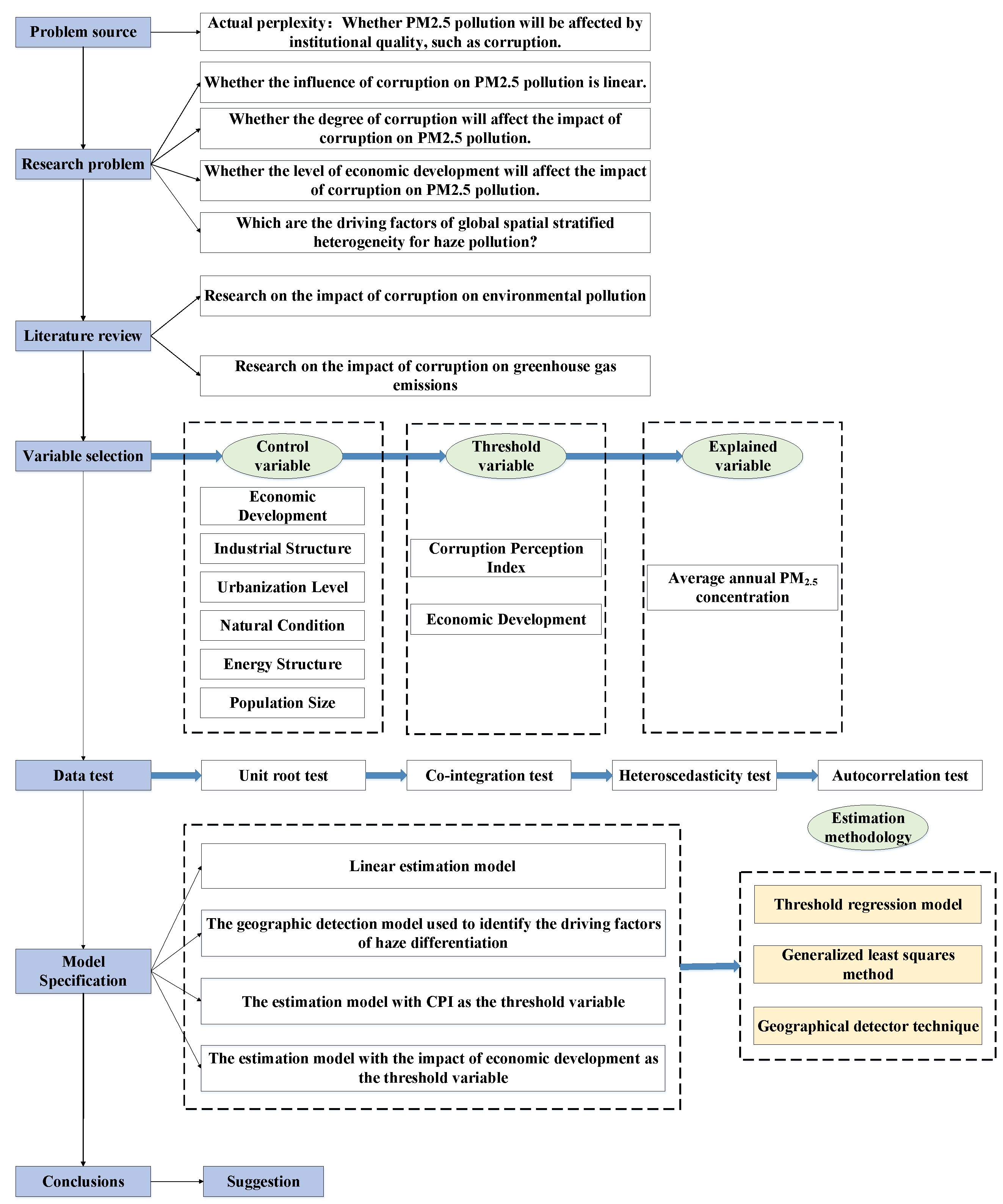
The relationship between corruption and economic development has long been the research focus of scholars. However, as global environmental issues have emerged, the analysis of how multiple factors affect environmental pollution has become a new research trend. As an intervention mechanism, political or institutional corruption (or both) attempt to avoid the restrictions of policies or even the formulation of policies through bribery or other means, and thus directly or indirectly affect the ecological environment of countries [32].

Corruption will directly deteriorate environmental quality through its effect on the strictness of environmental policies [33] and by weakening the strength of supervision [34]. However, factors such as people’s trust degree and the proportion of women with political power will ameliorate the negative effects of corruption [35]. For example, when the level of public trust is high, the negative impact of corruption on the strictness of environmental policies will be reduced, and may even show a positive correlation [36]. Environmental impact assessment is a key measure for alleviating the negative environmental impacts of development projects. If the process of environmental impact assessment is affected by corruption, the transparency, accountability, and participation of its application can no longer be guaranteed, thereby increasing the risk and uncertainty of the assessment [37,38]. Furthermore, corrupt countries receive less foreign direct investment than countries with respected governance systems, and the small amounts of foreign investment that are received mainly come from polluting enterprises seeking to minimize their outlay on pollution control [39,40]. Only countries that are based on democratic systems and minimize corruption can combine economic growth and pollution mitigation to achieve the sustained development of the economy and the environment simultaneously [41]. Corruption also affects environmental pollution through indirect effects. Taking SO₂ emissions as an example, the higher the level of corruption in a country, the higher the per capita income at the inflection point of the environmental Kuznets curve (EKC) [42].

With the intensification of the global greenhouse effect, controlling greenhouse gas emissions has become a major concern of various countries. Thus, research on the impact of the influence of corruption on greenhouse gas emissions is increasing. From a global perspective, Goel and Herrala [43] studied the factors influencing carbon emissions in 100 countries and concluded that the higher the level of corruption in a country, the lower its pollution level. However, this finding was contrary to results from a study of the Middle East and North Africa regions, which found that institutional quality had direct and indirect effects on the environment and these should be considered comprehensively to avoid estimation errors. Thus, different research objects lead to different conclusions. Sekrafi and Sghaier [44] researched 13 countries in the Middle East and North Africa and found that corruption hindered economic growth, thereby reducing CO₂ emissions. In Brazil, Russia, India, China, and South Africa, for example, corruption inhibited the promoting effect of economic growth on CO₂ emissions [45]. In 15 post-soviet independent countries, corruption directly affected CO₂ emissions, and also indirectly affected CO₂ emissions through per capita GDP. In these states, the indirect effect of corruption seemed to deserve more attention than the direct effects [46]. In Ghana, democracy directly reduced CO₂ emissions, which may indirectly reduce the emission effect brought by urbanization [32]. However, when further considering the impact of corruption on CO₂ emissions from various sectors, it was found that corruption increased the CO₂ emissions from the transportation sector, but manufacturing and construction helped reduce the carbon emissions [47]. Member countries of the Asia-Pacific Economic Cooperation forum also suffered from overall environmental degradation due to corruption. In countries with high CO₂ emissions, corruption did not affect emissions, but there was a significant promoting effect in countries with low CO₂ emissions [48]. Analyses of various countries in sub-Saharan Africa showed that democracy directly reduced CO₂ emissions and indirectly induced the emission-reducing effect of trade [49]; however, whether the institutional quality indirectly regulated the emission-reducing effect of energy consumption could not be verified [50].

Because of the advantages of the geographic detector model (GDM) in identifying the correlation between variables, this technique has been widely used to analyze the degree of independent variables to dependent variables since it was proposed [51]. Among them, GDM is mainly applied to the research of air pollution and human health [52,53]. Given this, we will apply GDM to verify this hypothesis, that is, there is a strong correlation between corruption and haze pollution.

Based on previous research, we propose a hypothesis that there may be a non-linear relationship between corruption and haze pollution, which can be tested by the threshold model. The threshold model mainly includes the static panel threshold model [54,55] and the dynamic panel threshold model [56,57], in which the static panel threshold model is mainly used to analyze the relationship between variables. At present, the threshold model has been widely used in the field of air pollution research. For example, taking China as an example, Wang et al. [58] analyzed the impact of economic growth and energy consumption structure on air quality.

The research framework is shown in Figure 1. Firstly, through the analysis of the relevant literature, the categories of influencing factors of smog pollution were determined. Secondly, we used the geographic detector model (GDM) to explore the explanatory degree of independent variables for haze pollution, which determined the following research focus. Thirdly, a threshold regression analysis framework was constructed to explore the non-linear relationship between corruption and haze pollution. Finally, we summarized the research conclusions and put forward the corresponding policy recommendations.

3. Methodology

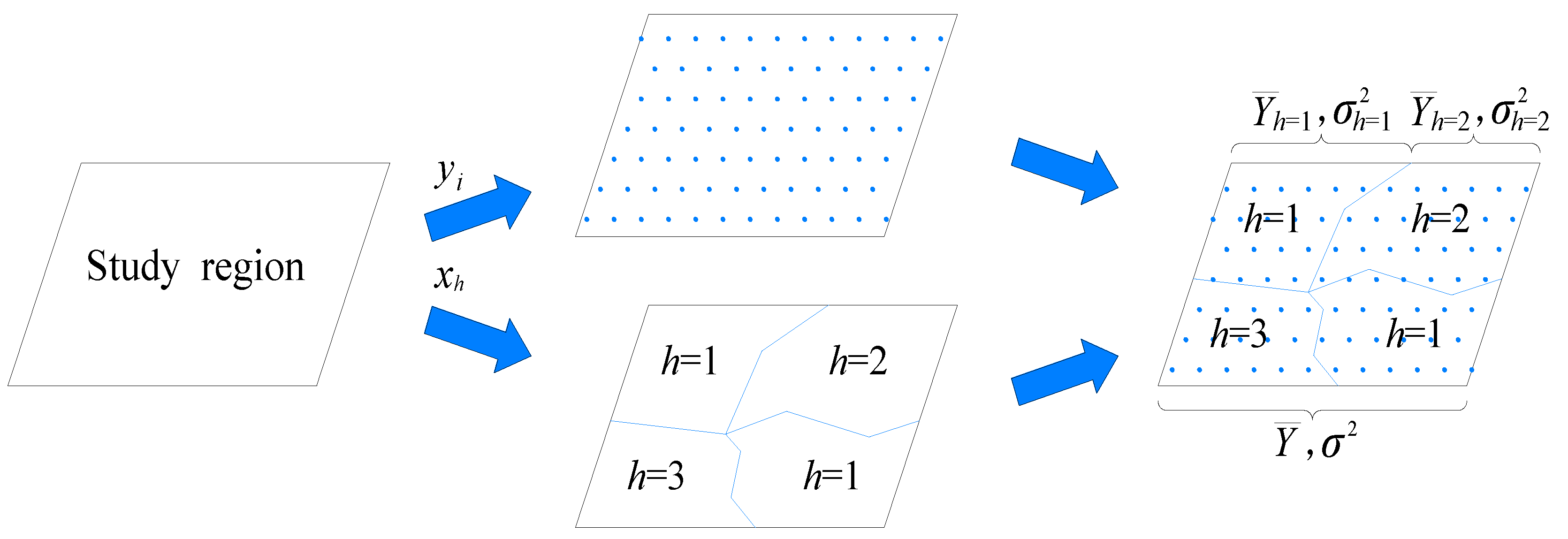
3.1. Geographical Detector Model

As is widely known, there are many factors affecting haze pollution. How to select the most influential independent variables has always been the focus of researchers. The geographical detector model helps us to choose the core influencing factors of haze pollution, which were proposed by Wang et al. [51]. As a statistical method, GDM not only explores the spatial differentiation of research objects but also reveals the driving force behind them. The core hypothesis of this technique is that if an independent variable has an important influence on a dependent variable, their spatial distribution should be similar [59]. By calculating the determinant power of the influencing factor (measured by q), we can explore the extent to which this influencing factor explains the spatial differentiation of the dependent variable [51]. Equation (1) is the specific expression of q [53]:

$$q=1-\frac{{{\displaystyle \sum }}_{h=1}^L{N}_h{\sigma }_h^2}{N{\sigma }^2}$$

(1)

N and $N_h$ represent the sample number of the whole region and the sample number of the sub-level region, respectively. h indicates the stratification of the dependent variable Y and factor X, and values range from one to L. ${\sigma }_h^2$ and ${\sigma }^2$ represent the variance of layers h and Y, respectively. The principle of geographical detector is shown in Figure 2. The value range of q is [0,1]. The larger the q value is, the stronger the explanatory power of independent variable X for dependent variable Y is, and vice versa. In extreme cases, when the q value is 1, it means that factor X completely controls the spatial distribution of Y; when the q value is 0, it means that X has nothing to do with Y.

The geographical detector model requires that the independent variable should be categorical data. Since the independent variable in this paper is a numerical quantity, the natural breaks classification method is first used for discretization. This method identifies the classification intervals, groups similar values most appropriately, and maximizes the differences between classes. ArcGIS software is used to classify driving factors in each year, which are mainly divided into four categories. Taking 2016 as an example, the classification of each factor is shown in

Table 1. Threshold values of dependent variables in 2016 by the natural breaks classification method.

Threshold	LnCPI	LnGDP	LnIS	LnURBAN	LnFOREST	LnEM	LnPOP
Level 1	[2.639,3.091]	[5.639,7.288]	[−3.952,−0.03891]	[−0.07162,2.013]	[−2.605,0.7265]	[−2.578,0.7168]	[0.6672,2.308]
Level 2	[3.092,3.689]	[7.289,8.716]	[−0.0389,1.826]	[2.014,3.202]	[0.7266,2.731]	[0.7169,2.580]	[2.309,3.846]
Level 3	[3.690,4.127]	[8.717,10.03]	[1.827,2.826]	[3.203,3.908]	[2.732,3.652]	[2.581,3.709]	[3.847,5.042]
Level 4	[4.128,4.500]	[10.04,11.52]	[2.827,4.271]	[3.909,4.414]	[3.653,4.430]	[3.710,4.679]	[5.043,8.976]

Note: square brackets “[” and “]” mean boundary values included. CPI: corruption perception index. GDP: economic development. IS: industrial structure. URBAN: urbanization. FOREST: natural environment. EM: energy mix. POP: population size.

below, and Figure 3 shows the spatial layout of the classification of seven influencing factors.

3.2. Linear Estimation Model

This study focused on the relationship between corruption and haze pollution. Considering the diversity of factors that influence haze pollution, some control variables are introduced to ensure a scientifically valid evaluation. The level of national economic development in a country is measured using per capita GDP. The industrial structure in each country is measured as the proportion of the added value of the tertiary industry to GDP. The environmental conditions in each country are assessed using the amount of forest area. The proportion of agricultural land in a country’s total land area is used as a measure of the level of urbanization. The energy mix is measured as the proportion of new-energy generation. The population size was measured by population density.

The PM_2.5 concentration in countries is taken as the explained variable, and the panel regression technique is adopted to fit the linear model (Equation (2)) to detect the effects of corruption and other factors on haze pollution:

$$\begin{gathered} LnP{M}_{2.5it}=\alpha LnCP{I}_{it}+{\beta }_{1}LnGD{P}_{it}+{\theta }_{1}LnI{S}_{it}+{\theta }_{2}LnFORES{T}_{it}+{\theta }_{3}LnURBA{N}_{it}+ \\ {\theta }_{4}LnE{M}_{it}+{\theta }_{5}LnPO{P}_{it}+{\mu }_i+{\epsilon }_{it} \end{gathered}$$

(2)

where $\alpha$ is the influence coefficient of the corruption perception index (CPI), ${\beta }_1$ and ${\theta }_n$ are the influence coefficient of each control variable, i represents the country, t represents the year, ${\mu }_i$ is the individual effect of each sample cross-section that did not change with time, and ${\epsilon }_{it}$ is the error term such that ${\epsilon }_{it}~iid\left(0,{\sigma }^2\right)$.

3.3. Estimation Model with CPI as the Threshold Variable

Based on Hansen’s panel threshold regression model, a basic model with CPI as the threshold variable was constructed to test the possible nonlinear characteristics between CPI and haze pollution at different CPI levels. Various control variables were introduced to develop the threshold estimation model used to identify the CPI independent variable effect:

$$\begin{gathered} LnP{M}_{2.5it}={\alpha }_{1}LnCP{I}_{it}\times I\left(LnCP{I}_{it}\le {\gamma }_1\right)+{\alpha }_{2}LnCP{I}_{it}\times I\left(LnCP{I}_{it}>{\gamma }_1\right)+\cdots \\ +{\alpha }_{2n-1}LnCP{I}_{it}\times I\left(LnCP{I}_{it}\le {\gamma }_n\right)+{\alpha }_{2n}LnCP{I}_{it}\times I\left(LnCP{I}_{it}>{\gamma }_n\right)+{\beta }_{1}LnGD{P}_{it}+{\theta }_{1}LnI{S}_{it}+ \\ {\theta }_{2}LnFORES{T}_{it}+{\theta }_{3}LnURBA{N}_{it}+{\theta }_{4}LnE{M}_{it}+{\theta }_{5}LnPO{P}_{it}+{\mu }_i+{\epsilon }_{it} \end{gathered}$$

(3)

In Equation (3), CPI_it is the core explanatory variable, indicating the corruption level of i country in year t. Meanwhile, CPI_it also serves as a threshold variable, indicating that the CPI level has different effects on haze pollution in different threshold intervals. $\mathsf{\gamma }$ is the threshold value of CPI to be estimated, which can be divided into two distinct areas. The regression coefficients of each area are different, which reflects the nonlinear characteristics between the degree of corruption and haze pollution. I (·) is the indicator function of the test hypothesis. When the condition in the brackets is satisfied, the hypothesis is met and I = 1; if the hypothesis is rejected then, I = 0.

3.4. Estimation Model with Economic Development as the Threshold Variable

To investigate the regulating effect of national economic development in various countries, economic development is introduced as the threshold variable into Equation (4), resulting in the threshold estimation model of the economic development effect.

$$\begin{gathered} LnP{M}_{2.5it}={\alpha }_{1}LnCP{I}_{it}\times I\left(LnGD{P}_{it}\le {\gamma }_1\right)+{\alpha }_{2}LnCP{I}_{it}\times I\left(LnGD{P}_{it}>{\gamma }_1\right)+\cdots \\ +{\alpha }_{2n-1}LnCP{I}_{it}\times I\left(LnGD{P}_{it}\le {\gamma }_n\right)+{\alpha }_{2n}LnCP{I}_{it}\times I\left(LnGD{P}_{it}>{\gamma }_n\right)+{\beta }_{1}LnGD{P}_{it}+{\theta }_{1}LnI{S}_{it} \\ +{\theta }_{2}LnFORES{T}_{it}+{\theta }_{3}LnURBA{N}_{it}+{\theta }_{4}LnE{M}_{it}+{\theta }_{5}LnPO{P}_{it}+{\mu }_i+{\epsilon }_{it} \end{gathered}$$

(4)

3.5. Variable Design

3.5.1. Explained Variables

Sulfur dioxide, nitrogen oxides, and inhalable particulate matter are the main components of haze. The former two are gaseous pollutants and inhalable particulate matter is the main culprit for aggravating hazy weather and pollution. PM_2.5 is especially considered to be the “prime criminal” of hazy weather. The annual average concentration of PM_2.5 in each country is used to represent the degree of haze pollution on an annual basis.

3.5.2. Core Explanatory Variables

In this study, corruption is taken to mean the act of abusing the rights of a public servant for personal benefit and can be divided into minor corruption and severe corruption [60,61,62]. Minor corruption means that people could avoid the negative effect of certain policies through bribery. Severe corruption denotes the bribing of politicians to influence the policies formulated [63]. Both minor corruption and severe corruption have an impact on environmental pollution [29]. While the impact of corruption on haze pollution has not yet reached a consensus, the effect of corruption on reducing the strictness of environmental policies has been widely recognized. Taking CO₂ emissions as an example, most studies showed that corruption increased CO₂ emissions from a global perspective. However, Halkons and Tzeremes [64] found that there was no linear relationship between corruption and CO₂ emissions and that better institutional quality did not necessarily lead to lower CO₂ emissions. The CPI of Transparency International is used in this study to measure the degree of corruption in each country. The higher the CPI value, the lower the degree of corruption, and vice versa.

3.5.3. Threshold Variables

The national CPI and per capita GDP are taken as the threshold variables to analyze whether the impact of corruption degree on haze pollution in the countries varies. Meanwhile, CPI is also regarded as a core explanatory variable.

Economic development: GDP reflects the level of economic development in a country, and environmental quality is always closely related to regional economic development. On the one hand, the rapid development of the economy requires a large amount of energy input, while the consumption of fossil energy will promote atmospheric emissions and cause haze pollution. On the other hand, rapid economic development can provide a government with a stable source of finance and taxation that can be used to increase investment in environmental protection and governance, thereby reducing haze pollution. The classic EKC hypothesis holds that as an economy grows, environmental quality initially tends to deteriorate, but then improves. Graphically, it depicts an inverted U-shaped curve. However, recent research has shown that a U-shaped, N-shaped or inverted N-shaped relationship might also exist between an environmental variable and economic growth [23]. Considering a country’s economic development status of haze pollution, per capita GDP is used as the control variable and threshold variable to measure the economic development level.

3.5.4. Control Variables

To obtain unbiased test results, five factors closely related to haze pollution are considered as control variables. The first of these is the industrial structure. Compared with fossil energy consumption and pollution emissions caused by the development of the secondary industry, the development of the tertiary industry is cleaner and has less impact on haze pollution. Therefore, the industrial structure is measured as the percent of value-added of the tertiary industry in GDP. The second control variable is urbanization. With the promotion of urbanization, built-up areas gradually expand and compress agricultural land, increasing the demand for housing and the use of motor vehicles, both of which degrade the environmental quality and exacerbate haze pollution. Therefore, the level of urbanization is measured as the proportion of agricultural land in a country’s total land area. The higher the proportion of agricultural land, the lower the level of urbanization. The third control variable reflects the natural environment. The characteristic of the natural environment is an important factor affecting environmental pollution; for example, the forested area can absorb 14 kg/m² of sulfur dioxide every year. Thus, the percentage of forest area in the national area is selected to measure the state of the natural environment of each country. The fourth control variable is the energy mix. Compared with the use of traditional fossil energy, new-energy has been recognized worldwide for its environmentally friendly and renewable characteristics. Considering that the burning of traditional fossil energy is one of the main factors causing haze pollution, the energy mix of any country will have an impact on haze pollution. The energy mix is included regarding Shao et al. [65] and Dong et al. [6], measured as the proportion of new energy generation in the total energy generation. The final control variable is the population size. Due to the large differences in the physical areas and populations of countries, there is no comparability in terms of the absolute value of population size. Therefore, with reference to the research of Shao et al. [23], the population density is used as the measure of population size in characterizing the impact of population aggregation on haze pollution.

3.6. Data

For the consistency of statistical caliber and the availability of data, 139 countries from 2010 to 2016 were selected as research objects. For the sample countries, the CPI data are mainly derived from Transparency International, and the other data are taken from the World Bank’s World Development Indicators.

Table 2. Descriptive statistics of variables.

Variables	Obs	Mean	Std. Dev	Min	Max
LnPM2.5	973	3.1716	0.6650	1.6412	5.3169
LnCPI	973	3.6632	0.4515	2.0794	4.5539
LnGDP	973	8.5733	1.4803	5.4459	11.6888
LnIS	973	1.9447	1.2089	−6.9525	4.2705
LnURBAN	973	3.5705	0.7353	−0.0716	4.4188
LnFOREST	973	2.9684	1.3105	−2.6547	4.4333
LnEM	973	2.8772	1.7041	−8.1266	4.6789
LnPOP	973	4.2661	1.2997	0.5752	8.9757

contains the descriptive statistical analysis of each variable.

4. Results and Discussion

4.1. Data Test

To avoid the interference of macroeconomic data having a temporal trend, a data stationarity test for variables was first conducted. Considering that the unit root process of each cross-section sequence of panel data might be different, the Levin–Lin–Chu (LLC) homogeneity test and the Im–Pesaran–Shin (IPS) heterogeneity test were selected for use. Under the two test methods, the original data of each variable did not completely reject the null hypothesis, but the first-order difference values of the variables rejected the null hypothesis under the LLC test. Under the IPS test method, only the ΔLnFOREST variable failed to pass the test. Overall, the variable panel data selected are the first-order stationary. To avoid the phenomenon of spurious regression in the model estimation, the Pedroni residual co-integration test tool was selected to analyze the co-integration relationship of panel data. The test results show that all statistical data passed the significance test at the 1% level. These results support the conclusion that there is a long-term stable equilibrium relationship among the selected variables.

Heteroscedasticity often occurs in actual economic data and will affect the estimation results from a model and increase the prediction error. Therefore, the White heteroscedasticity test was performed on the Equation (2). The test results show that Equation (2) rejects the null hypothesis of model homoscedasticity at the 1% significance level; consequently, it is deemed that heteroscedasticity existed in Equation (2). Due to the presence of autocorrelation in the data, the estimated fluctuation amplitude of the regression line based on the sample data has increased, resulting in inaccurate parameter estimation. An autocorrelation test was performed on Equation (2) using the Pesaran test. These results show that Equation (2) rejects the null hypothesis of the non-correlation of this model at the 1% significance level. Therefore, autocorrelation is deemed to exist in Equation (2). Thus, the generalized least squares estimation was used to test.

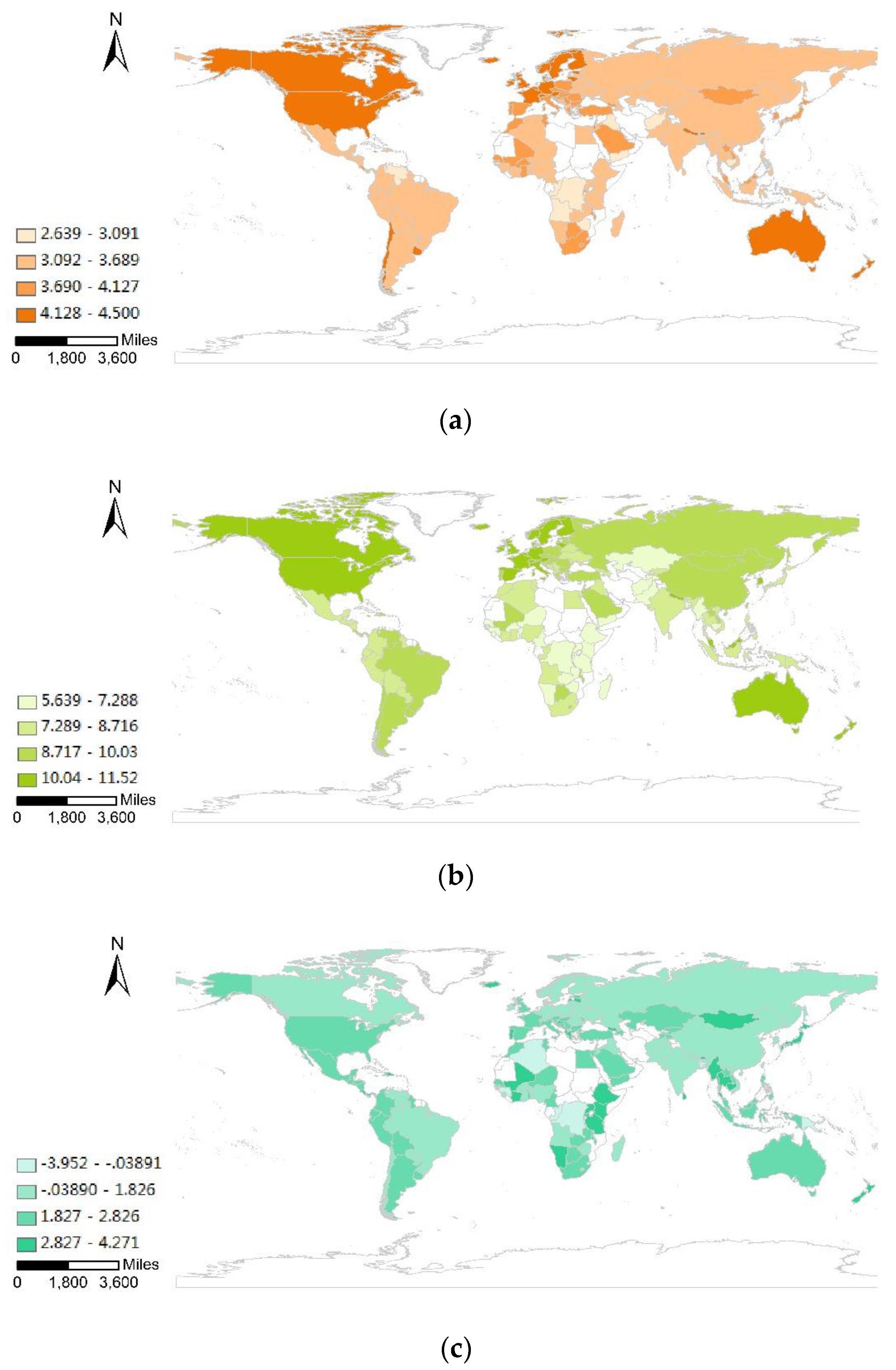
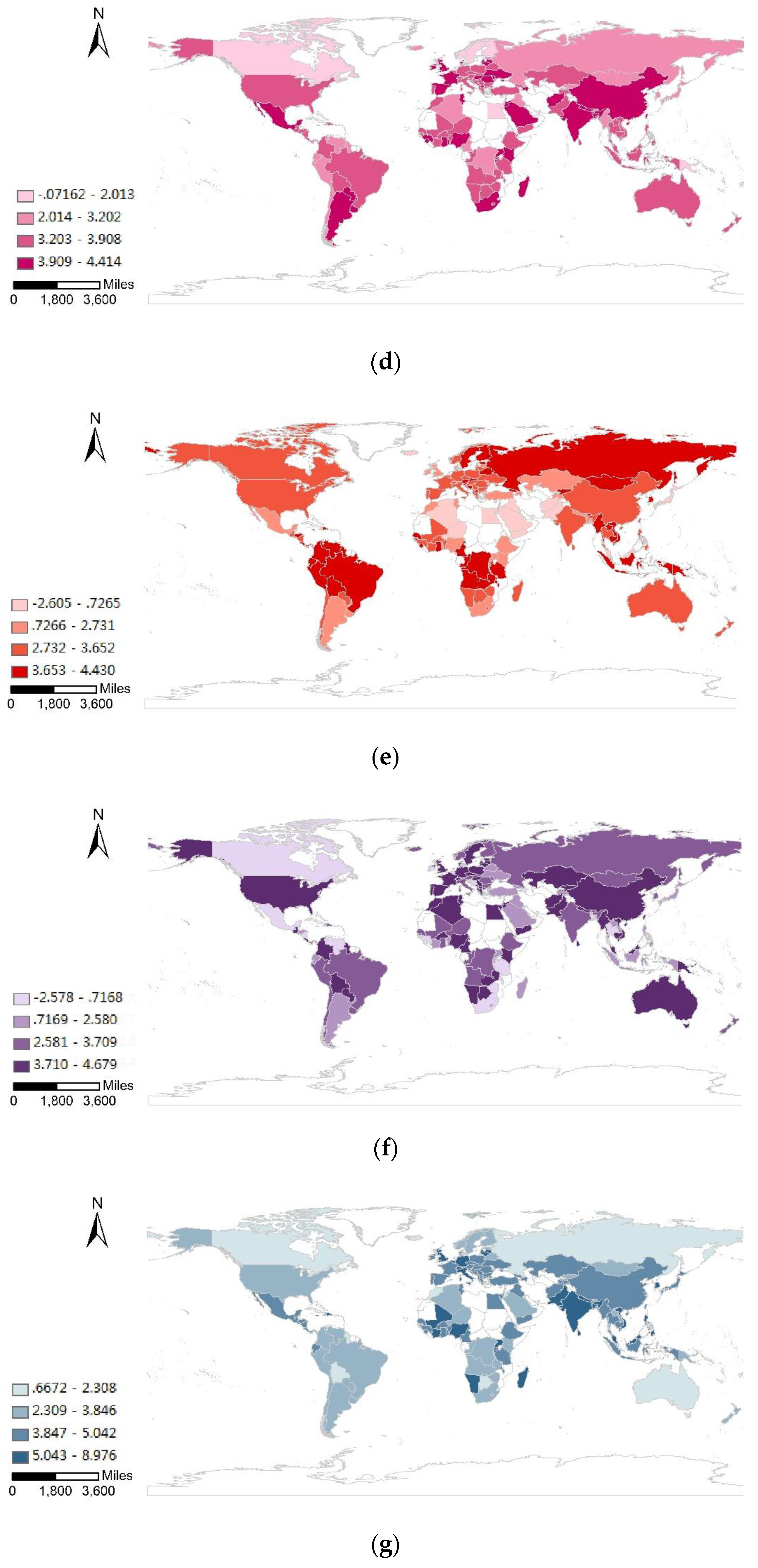
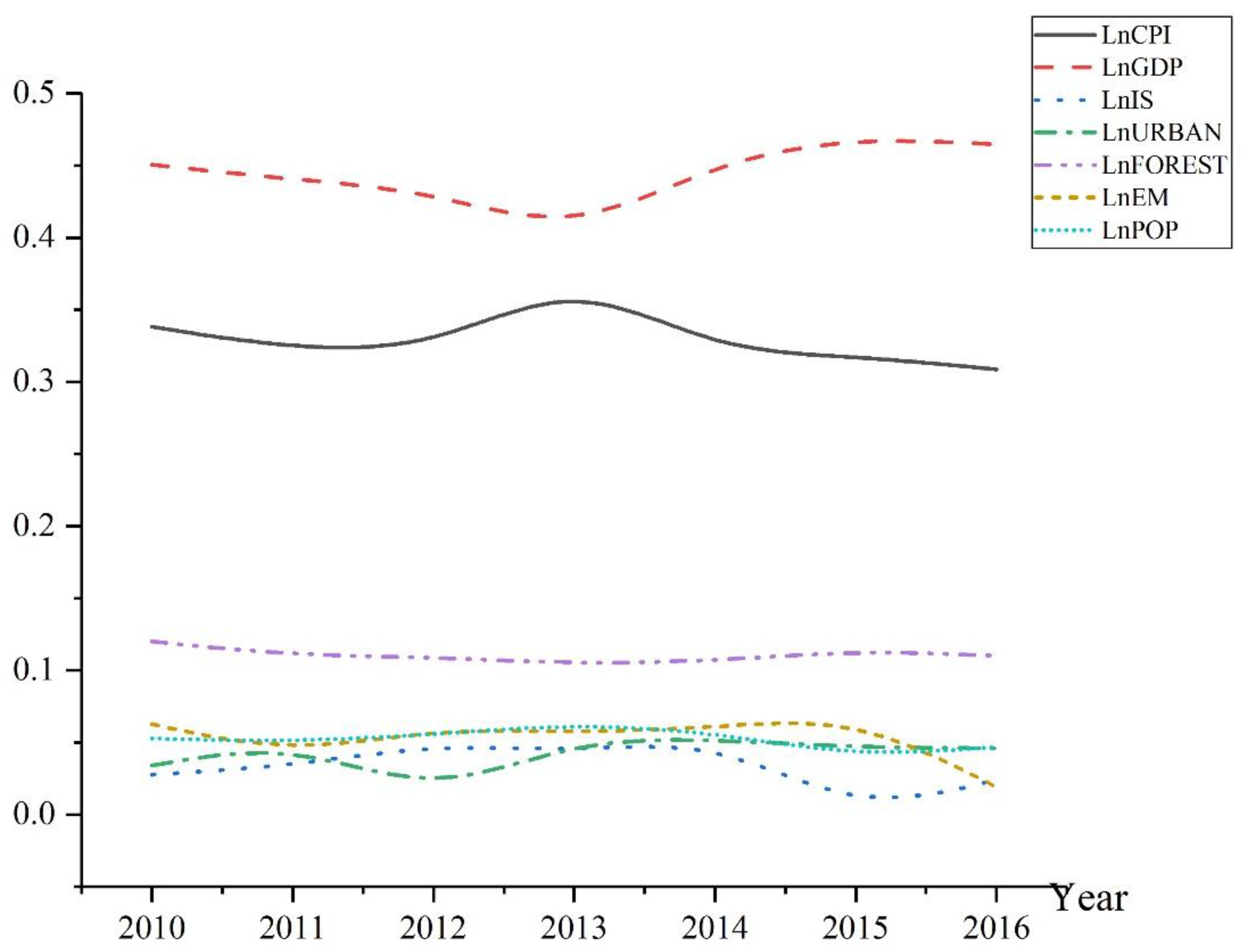
4.2. Driving Factors on PM_2.5 Concentrations

Seven indicators (namely, CPI, per capita GDP, industrial structure, urbanization, the natural environment, and the energy and population size) were chosen as the factor variables of geographical detection affecting haze pollution. Then, we used GDM to calculate the power of the determinant value of each independent variable for every year, and the specific results are shown in

Table 3. Power of determinant value of each driving factor from 2010 to 2016.

Year	LnCPI	LnGDP	LnIS	LnURBAN	LnFOREST	LnEM	LnPOP
2010	0.338123	0.450676	0.027602	0.034009	0.120013	0.062644	0.052929
2011	0.32281	0.440295	0.033695	0.050756	0.110451	0.041802	0.050312
2012	0.322874	0.432112	0.049083	0.012275	0.109273	0.059666	0.055528
2013	0.372594	0.4016	0.043365	0.052207	0.104586	0.056758	0.062916
2014	0.321366	0.453007	0.052688	0.052192	0.106432	0.060377	0.057164
2015	0.317953	0.469596	0.00112	0.046552	0.113855	0.068436	0.040022
2016	0.308656	0.46471	0.024016	0.046052	0.110196	0.01904	0.046906

below. Taking 2016 as an example, the order of influences of independent variables on spatial differentiation of haze pollution is GDP > CPI > FOREST > POP > URBAN > IS > EM. By plotting the q value distribution diagram of driving factors (see Figure 4), we find that although the influence of each factor on PM_2.5 pollution fluctuates, economic development, institutional quality, and natural environment are the main factors affecting haze pollution, among which economic development has the strongest explanatory power for haze.

Political factors are one of the main factors to explain the differences in global haze pollution. CPI accounts for the difference of PM_2.5 pollution in various countries to an extent from 30.87% to 37.29%. As a key factor affecting the economic development of a country, political factors have a huge impact not only on the national economy [66], but also on the ecological environment [63,67]. Data shows that countries with severe corruption usually face serious environmental problems. The process of haze pollution control forces the construction and improvement of the national system, while the alleviation of corruption maximizes the effectiveness of haze pollution control. Despite how economic development affects environmental pollution has always been a hotly debated topic [68], there is no denying that a country’s wealth is extremely important to the environment. Taking haze pollution as an example, economic development accounted for 40.16% to 46.96% of the difference in haze pollution among different countries. Although the EKC hypothesis has been verified in some countries, most countries are currently in the stage of a negative correlation between economic development and haze pollution in terms of global development trends. Specifically, for countries at different stages of economic development, the relationship between per capita GDP and haze pollution is different. Considering the importance of economic development in haze pollution control, middle-income countries should further accelerate economic development to achieve a win-win situation of ecological environment and economic development. In addition to CPI and GDP, the natural environment also accounted for the difference in haze pollution, and the explanation is maintained at about 10%, which shows that afforestation is also the key method to alleviate haze pollution.

Although the seven factors we selected have a significant relationship with haze pollution, only three variables (namely CPI, GDP, and FOREST) had a strong explanation for haze. This indicates that changes in the industrial structure, urbanization rate, energy mix and population density of a given country all bring about fluctuations of PM_2.5 concentration, but these factors were not the main reasons for the differences in global haze pollution. From a macroscopic perspective, improving national system construction, accelerating national economic development and building a harmonious ecological environment are the keys to shorten the gap of haze pollution between countries.

4.3. Model Estimation Results with CPI as the Threshold Variable

Before using the threshold model, we should check whether there is a threshold point in the model, that is, the threshold effect test. Generally speaking, the results of the threshold effect test provide a basis for whether the threshold model should be used. According to Hansen’s theory of threshold regression [69], the samples were first arranged in ascending order by the threshold variable. The “grid search method” is used continuously to yield the candidate threshold value η in the threshold regression. Regressions are conducted for each threshold, and the residual sum of squares S1(η) of the corresponding model is calculated. The minimum value as S1(η) was selected to obtain the estimated value η as the actual threshold value of model estimation. The likelihood ratio is simulated using the “bootstrap method” and all the statistical data are simulated 1000 times. The bootstrap p value of the threshold existence test is obtained from these simulations. As shown in

Table 4. Threshold estimation and threshold test of Equation (3).

Threshold Model	Threshold Test	Estimated Value	95% Confidence Interval	F Value	p-Value	Bootstrap Times
Threshold model with CPI as the threshold variable	Single threshold	2.9038	[2.8470,3.0361]	10.0385	0.0000	1000
	Double threshold	3.2252	[2.6391,4.5109]	3.8205	0.0660	1000
	Triple threshold	3.5088	[2.6391,4.5109]	5.3118	0.0250	1000

, Equation (3) passes at the 10% significance level of the single threshold (2.9038), the double threshold, and the triple threshold; meanwhile, the 95% confidence interval of the triple-threshold is [2.6391,4.5109], which indicates that the effect of corruption on haze pollution exhibited significant triple-threshold characteristics.

To facilitate system analysis and comparison, the threshold effects for all countries are estimated first, and then the samples are divided into four types of countries based on the estimated threshold effect of the CPI independent variable. The four categories are “severely corrupt”, “moderately corrupt”, “slightly corrupt”, and “non-corrupt”. Despite the fact that the nonlinear relationship between haze pollution and corruption can be explored by using the high-order function or threshold model, there is significant multicollinearity in the high-order function. At the same time, Equation (3) passed the threshold effect test, indicating that the panel threshold model should be used. Considering the heteroscedasticity and autocorrelation of the panel data, the generalized least squares method is used to estimate the model. The results are shown in

Table 5. Parameter estimating results when taking CPI as a threshold variable.

Variables	Overall	Severely Corrupt	Moderately Corrupt	Slightly Corrupt	Non-Corrupt
LnCPI	−0.1217 *** (−4.35)	0.0299 (0.18)	−0.0237 (−0.11)	−0.9179 *** (−5.21)	−0.2243 *** (−6.69)
LnGDP	−0.2302 *** (−20.94)	−0.2667 *** (−5.16)	−0.1768 *** (−12.61)	−0.2598 *** (−18.30)	−0.3255 *** (−38.33)
LnIS	−0.0205 *** (−2.96)	−0.1684 *** (−5.13)	−0.0487 *** (−4.02)	−0.0661 *** (−4.63)	−0.1135 *** (−12.94)
LnURBAN	−0.0239 (−1.45)	−0.5572 *** (−6.00)	−0.0617 (−1.45)	−0.1859 *** (−11.80)	−0.0263 *** (−3.01)
LnFOREST	−0.1354 *** (−12.13)	−0.1711 *** (−7.57)	−0.0774 *** (−3.09)	−0.1460 *** (−22.53)	−0.0911 *** (−9.84)
LnEM	−0.0015 (−0.56)	−0.0889 *** (−2.95)	−0.0309 ** (−2.48)	−0.0202 ** (−2.54)	−0.0532 *** (−10.90)
LnPOP	0.0797 *** (8.22)	−0.2447 *** (−5.62)	0.1155 *** (5.70)	0.1701 *** (15.26)	0.0854 *** (18.31)
Constant	5.7385 *** (48.37)	9.6933 *** (12.57)	4.9416 *** (7.31)	9.0741 *** (16.00)	7.2687 *** (66.64)
Obs	973	29	139	221	584

Note: Z-values are reported in parentheses. * indicates p < 0.1; ** indicates p < 0.5; *** indicates p < 0.01.

. In particular, according to the results of the Hausman test, we have considered the country fixed effect in the model estimation.

The institutional quality of a country is one of the main factors affecting air pollution. Considering the total sample, the CPI is negatively correlated with haze pollution [70]. However, each country’s national conditions are different and the impact of corruption degree on haze pollution showed a significant nonlinear relationship. Thus, it cannot be concluded that suppressing corruption is an ideal approach to solving haze pollution problems. Instead, it is necessary to explore the relationship between corruption and haze pollution while considering countries with different corruption degrees [64].

In countries with different degrees of corruption, factors differ in their influence on haze pollution. In countries where corruption is severe, the suppression of corruption has an increasing effect on haze pollution, though this effect is not significant. The cause of the phenomenon may be that severe corruption distorted the national economy [44,71]. When a country starts to control the degree of corruption, it usually first focuses on its economic development issues and neglects the governance of atmospheric and other types of pollution. Thus, efforts to control corruption in a severely corrupt country exacerbated haze pollution in the short term. Moreover, for countries with severe corruption, bribery has affected the statistical data that measured environmental pollution, making the haze pollution data inconsistent with reality to avoid the punishment of environmental policies [72]. Therefore, when the corrupt behavior is controlled, the concentrations of pollutants appear to increase because they were under-reported previously.

For countries with a moderate degree of corruption, the governance of corrupt behavior has produced an inhibitory effect on haze pollution, but this effect was not obvious. In countries with minor corruption and non-corruption, the influence coefficient of CPI on haze pollution passed the 1% significance test; thus, it had an inhibitory effect on haze pollution. This result indicates that for countries with relatively high levels of institutional quality, the implementation of environmental policies is relatively strong, and the impact of corruption on the implementation of environmental policies is relatively weak. Further improving the institutional quality and ensuring the implementation of environmental policies are the keys to alleviating haze pollution.

It is worth noting that when a country is in a state of minor corruption, the effect of improving the institutional quality and suppressing corruption on the reduction of haze pollution is more obvious. Despite that, for a country without corruption, this effect is greatly reduced, which indicates that the relationship between institutional quality and haze pollution can be represented by diminishing marginal returns. Relatively honest countries may face more problems in terms of environmental management to a lesser extent than corrupt countries. Although the execution efficiency of the public sector will increase in an honest country [73], more attempts are required for a government during the development of environmental policies to balance the interests of different stakeholders. The extra time required to enact policies reduces the impact of corruption control on haze pollution, at least in the short and medium-term.

The development and protection of the ecological environment have been valued by various countries around the world. A relatively high level of economic development will significantly inhibit haze pollution. Both in the total sample or when grouped according to their degrees of corruption, the decoupling of economic development from haze pollution has been a major trend [74]. The secondary industry is one of the main causes of haze pollution. With the end of industrialization in many countries, the arrival of the information age has accelerated the development of the tertiary industry and gradually formed an industrial structure dominated by this advanced industry. The increase in the proportion of the tertiary industry will significantly alleviate haze pollution [75]. Despite the fact that the increase of agricultural land has also played a certain role in alleviating haze pollution, this effect is not significant. However, in countries with different degrees of corruption, it has greatly varied the impact of urbanization on haze pollution [15]. Conditions associated with the natural environment are one key to alleviating haze pollution. For countries plagued by haze pollution, strengthening environmental supervision is also essential to avoiding haze pollution. Meanwhile, faced with the need to remediate polluted air, increasing the vegetation-planting rate will greatly reduce haze pollution.

Globally, changes in the energy mix will not significantly affect haze pollution. Among countries with different institutional quality levels, it was found that the impact of the rising proportion of new-energy consumption on haze pollution passed the significance test. In general, the dominance of fossil energy as the main source of energy supply is one of the main causes of PM_2.5 [76]. Yet the mitigation effect of a clean energy consumption structure on haze pollution is weak, mainly because using of new-energy currently was not promoted globally and the traditional fossil energy is still key to supporting economic development. The size of the population is a major factor contributing to haze pollution. Countries with high population density usually generate a great demand for housing, home appliances, and motor vehicles, all of which were the main causes of haze pollution. In addition, traffic congestion caused by population agglomeration is not conducive to the efficient combustion of motor vehicle fuel, which exacerbates atmospheric pollution. Meanwhile, high residential density affects wind speed and is not conducive to the diffusion of pollutants, thereby indirectly aggravating haze pollution. However, in countries with severe corruption, the increase of population density has a typical agglomeration effect, which improves the proportion of public transport in the overall travel modes of citizens and the efficiency of resource use, thereby reducing air pollution to some extent [77].

There was a typical nonlinear relationship between the degree of corruption and haze pollution. When the degree of corruption of a country changes, the impact of CPI on PM_2.5 concentration also changes. It is important to examine whether the level of economic development also regulates the relation between CPI and haze pollution.

4.4. Model Estimation Results with Economic Development as the Threshold Variable

In order to analyze the relationship between corruption and haze pollution in countries with different economic development levels, the threshold test was first conducted, and the results are shown in

Table 6. Threshold estimation and threshold test of Equation (4).

Threshold Model	Threshold Test	Estimated Value	95% Confidence Interval	F Value	p-Value	Bootstrap Times
Threshold model with GDP as the threshold variable	Single threshold	6.6991	[6.3313,10.8825]	6.5384	0.0130	1000
	Double threshold	7.4346	[7.3887,7.4346]	10.8009	0.0000	1000
	Triple threshold	7.7105	[6.3313,10.8825]	4.9255	0.0190	1000

below. Equation (4) passed the 5% significance level test of the single threshold, double threshold, and triple threshold, and the 95% confidence interval of the triple-threshold is [6.3313,10.8825]. This result indicates that the impact of corruption on haze pollution was affected by the level of economic development [78].

To facilitate system analysis and comparison, the threshold effects for all countries were estimated first. Then, based on the threshold effect estimates, the total sample countries were divided into four types based on their level of economic development: “low income”, “middle-low income”, “middle-high income”, and “high income”. The generalized least squares method was adopted and the country fixed effect was considered. The results are shown in

Table 7. Parameter estimating results when taking GDP as a threshold variable.

Variables	Overall	Low Income	Middle-Low Income	Middle-High Income	High Income
LnCPI	−0.1217 *** (−4.35)	0.1606 ** (2.39)	0.5143 *** (6.26)	−0.0878 (−0.30)	−0.1472 *** (−5.41)
LnGDP	−0.2302 *** (−20.94)	0.2636 *** (3.45)	0.2701 *** (3.01)	−0.6647 (−1.35)	−0.3113 *** (−28.82)
LnIS	−0.0205 *** (−2.96)	−0.010 (−0.87)	−0.1900 *** (−12.06)	−0.0151 (−0.27)	−0.0668 *** (−8.26)
LnURBAN	−0.0239 (−1.45)	−0.5070 *** (−9.75)	−1.0436 *** (−15.14)	−0.0303 (−0.31)	0.0157* (1.74)
LnFOREST	−0.1354 *** (−12.13)	−0.2477 *** (−10.10)	−0.1511 *** (−14.60)	−0.2274 *** (−5.87)	−0.1555 *** (−17.55)
LnEM	−0.0015 (−0.56)	−0.0936 *** (−6.76)	−0.0718 *** (−6.87)	0.1422 *** (3.26)	−0.0244 *** (−5.66)
LnPOP	0.0797 *** (8.22)	0.1493 *** (6.92)	0.2707 *** (15.62)	−0.0371 (−1.51)	0.0980 *** (20.93)
Constant	5.7385 *** (48.37)	3.9297 *** (7.86)	3.6788 *** (5.06)	9.318 ** (2.34)	6.6315 *** (79.51)
Obs	973	131	129	44	669

Note: Z-values are reported in parentheses. * indicates p < 0.1; ** indicates p < 0.5; *** indicates p < 0.01.

.

In various national economic developments, the impact of institutional quality on haze pollution differs noticeably [79]. Contrary to the results when all countries are analyzed collectively, the threshold effect test for different groups of countries produced the following results. First, when the per capita GDP was in the low and middle-low ranges, a reduction of corruption significantly increases the concentration of atmospheric PM_2.5. The main reason for this phenomenon is that economic development is the priority for low income and middle-low income countries. For lesser-developed countries without a vibrant tourism industry, it is almost impossible for the national governments to consider both economic development and environmental protection. Therefore, even relatively honest low-income countries tend to choose to develop their national economies first and give environmental protection a lower priority. This prioritization was an important factor leading to aggravated haze pollution.

Second, as national economies develop, CPI is negatively correlated with haze pollution. However, when the per capita income is in the middle and high ranges, the influence coefficient of the CPI on haze pollution is −0.0878, and the p-value is 0.767, indicating that the effect of controlling corruption on the suppression of haze pollution was not significant.

Third, in countries with highly developed national economies, the influence coefficient of CPI on haze pollution is −0.1472, and it passes the significance test at the 1% level, indicating that for countries with high national income, fighting corruption and maintaining a high level of institutional quality had a significant inhibitory effect on haze pollution. This result occurred mainly because the citizens in countries with developed economies have high demands for good air quality and a high-quality ecological environment [79]. A relatively more honest country will fully consider the environmental demands of citizens, place economic development and environmental protection in equally important positions, and introduce more environmental policies that are stringent and effective.

Contrary to the impact of per capita GDP on haze pollution in the total pool of all 139 countries, there is a significant nonlinear relationship between the level of economic development and haze pollution when countries are grouped according to economic development [80]. For low income and middle-low income countries, the inflection points of the EKC were not passed during the study period. The level of economic development in these countries is positively related to the degree of smog pollution, and the development of the national economy induced haze pollution. For high-income countries, the inflection points of the EKC were crossed. In these countries, economic development is significantly negatively correlated with haze pollution and abundant national capital plays an important role in haze control. Moreover, the level of economic development also promotes the effect of institutional quality on haze pollution and indirectly eases the degree of haze pollution in high-income countries. The results show that the direct and indirect reducing effect of the national economy on PM_2.5 pollution is significant, and accelerating economic development is also one of the keys to promoting the mitigation of haze pollution [81].

The study finds that the level of economic development significantly influenced the PM_2.5 concentration effect on corruption; a higher level of national economy not only eases the haze pollution directly but also indirectly promotes the institutional quality of smog pollution inhibition. The “Matthew effect” is further manifested; that is, the higher the level of economic development, the lower the haze pollution level.

5. Conclusions and Policy Implications

5.1. Conclusions

This study of 139 countries considered the impact of institutional quality on environmental quality. More specifically, the research examined the impact of the CPI on haze pollution. A nonlinear relationship between corruption and haze pollution was observed. Mathematical models were developed to analyze this relationship, first by considering the degree of corruption as a threshold variable and then by using the level of economic development as the threshold variable. Total sample countries were then divided based on the estimated threshold effects so that the factors influencing haze pollution in different groupings of countries could be further analyzed. Three main conclusions were supported by the study results.

(1)

On a global basis considering all 139 countries collectively, the CPI was significantly negatively correlated with haze pollution. The power of determination for CPI was relatively high and stable during the observation period, indicating that political factors were one of the key factors contributing to the stratification heterogeneity of global haze pollution. However, this should not be interpreted to mean that severer corruption universally results in more haze pollution. With the improvement of the quality of the national system and the reduction of corruption, the implementation and stringency of local environmental policies also improve, and the implementation of these policies becomes more certain, which greatly alleviates haze pollution. However, in this study, the impact of the degree of corruption on haze pollution showed significant triple threshold characteristics. That is, when corruption in a country was severe, the mitigation of corruption did not affect haze pollution. Yet when the CPI crossed the double threshold value, the strengthening of institutional quality significantly inhibited haze pollution.

(2)

As the main factor causing spatial heterogeneity of PM_2.5 concentration, per capita GDP was also an important indicator for measuring the national economic level, which significantly adjusted the impact of institutional quality on haze pollution. In countries with high incomes, choosing a ruling party that is less susceptible to corruption significantly reduced haze pollution and created an ecological environment that is more suitable for civil life. Nevertheless, in low-income countries, an honest government will not significantly inhibit haze pollution; on the contrary, it appears to greatly exacerbate a country’s haze pollution. However, the aggravated level of pollution may be apparent rather than actual, given that pollution monitoring in low-income, politically corrupt countries is unreliable.

(3)

When countries economic development was at a relatively high level, per capita GDP had an inhibitory effect on haze pollution, not only indirectly through the moderating effects of lifestyle changes and public demand for a high-quality environment, but also directly through efficiency improvements in the energy mix. The “Matthew effect” was manifested in the international community such that the higher the level of economic development, the lower was the severity of haze pollution.

5.2. Policy Implications

The influence of political factors and economic development level on haze pollution was mainly considered in this study. Based on the research results, the following recommendations are proposed to alleviate global haze pollution pressure.

(1)

Strengthen the construction of environmental institutions and anti-corruption institutions and ensure probity during the institution implementation process. All countries should actively promote the construction of environmental institutions. Countries should not only comprehensively rectify defects in the existing institutions, highlight the key points of environmental institution construction, and improve institutional quality, but also develop environmental institutions into a respected scientific and rational institutional system. To ensure the effect of implementing the environmental system, national governments should actively introduce anti-corruption laws and regulations and strengthen the supervision of the implementation process of the institutional environmental system. In summary, national governments must prevent corruption from reducing the effectiveness of an environmental system, ensure the effectiveness of institutional construction, strengthen the awareness of national laws and regulations, and strengthen the publicity and education about anti-corruption systems, so as to alleviate the pressure of PM_2.5 pollution.

(2)

Upgrade the industrial structure, accelerate economic development, and give full play to the haze-reducing effect of the national economy. First, efforts should be made to improve the industrial structure by promoting the development of less-polluting types of industry, increase support for the financial industry, service industry and high technology industries, strengthen environmental supervision of the production process of the secondary industry, and curb the emission of PM_2.5 at the source. Second, national governments are supposed to promote the upgrading of the industrial structure in order to improve the comprehensive competitiveness of the national economy, give full play to a high level of economic development for its direct and indirect effects in reducing haze pollution, increase haze control investment, and ensure the benefits of PM_2.5 pollution control.

References

1. Dong, F.; Dai, Y.; Zhang, S.; Zhang, X.; Long, R. Can a carbon emission trading scheme generate the Porter effect? Evidence from pilot areas in China. Sci. Total Environ. 2019, 653, 565–577. [Google Scholar] [CrossRef]
2. Dong, F.; Wang, Y.; Zheng, L.; Li, J.; Xie, S. Can industrial agglomeration promote pollution agglomeration? Evidence from China. J. Clean. Prod. 2019, 246, 118960. [Google Scholar] [CrossRef]
3. Dong, F.; Li, J.; Li, K.; Sun, Z.; Yu, B.; Wang, Y.; Zhang, S. Causal chain of haze decoupling efforts and its action mechanism: Evidence from 30 provinces in China. J. Clean. Prod. 2019, 245, 118889. [Google Scholar] [CrossRef]
4. Word Health Organization. 2018. Available online: http://www.who.int/news-room/fact-sheets/detail/ambient-(outdoor)-air-quality-and-health (accessed on 2 May 2018).
5. Air Pollution in World. Air Pollution in World: Real-Time Air Quality Index Visual Map. 2019. Available online: http://aqicn.org/map/world (accessed on 14 January 2019).
6. Dong, F.; Li, J.; Wang, Y.; Zhang, X.; Zhang, S.; Zhang, S. Drivers of the decoupling indicator between the economic growth and energy-related CO2 in China: A revisit from the perspectives of decomposition and spatiotemporal heterogeneity. Sci. Total Environ. 2019, 685, 631–658. [Google Scholar] [CrossRef] [PubMed]
7. Joss, M.K.; Eeftens, M.; Gintowt, E.; Kappeler, R.; Künzli, N. Time to harmonize national ambient air quality standards. Int. J. Public Health 2017, 62, 453–462. [Google Scholar] [CrossRef] [PubMed] [Green Version]
8. Dong, F.; Wang, Y.; Su, B.; Hua, Y.; Zhang, Y. The process of peak CO2 emissions in developed economies: A perspective of industrialization and urbanization. Resour. Conserv. Recy. 2019, 141, 61–75. [Google Scholar] [CrossRef]
9. Xie, Y.; Dai, H.; Dong, H.; Hanaoka, T.; Masui, T. Economic impacts from PM2.5 pollution-related health effects in China: A provincial-level analysis. Environ. Sci. Technol. 2016, 50, 4836–4843. [Google Scholar] [CrossRef]
10. Shou, Y.K.; Huang, Y.L.; Zhu, X.Z.; Liu, C.Q.; Hu, Y.; Wang, H.H. A review of the possible associations between ambient PM2.5 exposures and the development of Alzheimer’s disease. Ecotoxicol. Environ. Saf. 2017, 174, 344–352. [Google Scholar] [CrossRef]
11. Baasandorj, M.; Hoch, S.W.; Bares, R.; Lin, J.C.; Brown, S.S.; Millet, D.B.; Martin, R.; Kelly, K.; Zarzana, K.J.; Whiteman, C.D. Coupling between chemical and meteorological processes under persistent cold-air pool Conditions: Evolution of wintertime PM2.5 pollution events and N2O5 observations in Utah’s Salt Lake Valley. Environ. Sci. Technol. 2017, 51, 5941–5950. [Google Scholar] [CrossRef]
12. Chen, Y.; Schleicher, N.; Cen, K.; Liu, X.; Yu, Y.; Zibat, V.; Dietze, V.; Fricker, M.; Kaminski, U.; Chen, Y. Evaluation of impact factors on PM2.5 based on long-term chemical components analyses in the megacity Beijing, China. Chemosphere 2016, 155, 234–242. [Google Scholar] [CrossRef]
13. Ming, L.L.; Jin, L.; Li, J.; Fu, P.Q.; Yang, W.Y.; Liu, D.; Zhang, G.; Wang, Z.F.; Li, X.D. PM2.5 in the Yangtze River Delta, China: Chemical compositions, seasonal variations, and regional pollution events. Environ. Pollut. 2017, 223, 200–212. [Google Scholar] [CrossRef]
14. Styszko, K.; Samek, L.; Szramowiat, K.; Korzeniewska, A.; Kubisty, K.; Rakoczy-Lelek, R.; Kistler, M.; Giebl, A.K. Oxidative potential of PM10 and PM2.5 collected at high air pollution site related to chemical composition: Krakow case study. Air Qual. Atmos. Health 2017, 10, 1123–1137. [Google Scholar] [CrossRef]
15. Ji, X.; Yao, Y.X.; Long, X.L. What causes PM2.5 pollution? Cross-economy empirical analysis from socioeconomic perspective. Energy Policy 2018, 119, 458–472. [Google Scholar] [CrossRef]
16. Wu, J.; Zhang, P.; Yi, H.; Qin, Z. What causes haze pollution? An empirical study of PM2.5 concentrations in Chinese cities. Sustainability 2016, 8, 132. [Google Scholar] [CrossRef] [Green Version]
17. Zhang, Y.; Shuai, C.Y.; Bian, J.; Chen, X.; Wu, Y.; Shen, L.Y. Socioeconomic factors of PM2.5 concentrations in 152 Chinese cities: Decomposition analysis using LMDI. J. Clean. Prod. 2019, 218, 96–107. [Google Scholar] [CrossRef]
18. Xu, G.Y.; Ren, X.D.; Xiong, K.N.; Li, L.Q.; Bi, X.C.; Wu, Q.L. Analysis of the driving factors of PM2.5 concentration in the air: A case study of the Yangtze River Delta, China. Ecol. Indic. 2020, 110, 105889. [Google Scholar] [CrossRef]
19. Zhou, Q.L.; Wang, C.X.; Fang, S.J. Application of geographically weighted regression (GWR) in the analysis of the cause of haze pollution in China. Atmos. Pollut. Res. 2019, 10, 835–846. [Google Scholar] [CrossRef]
20. Grossman, G.M.; Krueger, A.B. Economic growth and the environment. Q. J. Econ. 1995, 110, 353–377. [Google Scholar] [CrossRef] [Green Version]
21. Luo, K.; Li, G.; Fang, C.; Sun, S. PM2.5 mitigation in China: Socioeconomic determinants of concentrations and differential control policies. J. Environ. Manag. 2018, 213, 47–55. [Google Scholar] [CrossRef]
22. Liu, J.K.; Yan, G.X.; Wu, Y.N.; Wang, Y.; Zhang, Z.M.; Zhang, M.X. Wetlands with greater degree of urbanization improve PM2.5 removal efficiency. Chemosphere 2018, 207, 601–611. [Google Scholar] [CrossRef]
23. Shao, S.; Li, X.; Cao, J.H.; Yang, L.L. Economic policy choice for haze pollution control in China—based on the perspective of spatial spillover effect. Econ. Res. 2016, 51, 73–88. (In Chinese) [Google Scholar]
24. Bari, M.A.; Kindzierski, W.B. Fine particulate matter (PM2.5) in Edmonton, Canada: Source apportionment and potential risk for human health. Environ. Pollut. 2016, 218, 219–229. [Google Scholar] [CrossRef] [PubMed]
25. Steinhardt, H.C.; Wu, F. In the name of the public: Environmental protest and the changing landscape of popular contention in China. China J. 2016, 75, 61–82. [Google Scholar] [CrossRef] [Green Version]
26. Cao, X.; Kostka, G.; Xu, X. Environmental political business cycles: The case of PM2.5 air pollution in Chinese prefectures. Environ. Sci. Policy 2019, 93, 92–100. [Google Scholar] [CrossRef]
27. Romuald, K.S. Democratic institutions and environmental quality: Effects and transmission channels. In Proceedings of the International Congress, European Association of Agricultural Economists, Zurich, Switzerland, 30 August–2 September 2011. [Google Scholar]
28. Wang, N.L.; Zhu, H.M.; Guo, Y.W.; Peng, C. The heterogeneous effect of democracy, political globalization, and urbanization on PM2.5 concentrations in G20 countries: Evidence from panel quantile regression. J. Clean. Prod. 2018, 194, 54–68. [Google Scholar] [CrossRef]
29. Arminena, H.; Menegakibc, A.N. Corruption, climate and the energy-environment-growth nexus. Energy Econ. 2019, 80, 621–634. [Google Scholar] [CrossRef]
30. Lemprière, M. Using ecological modernisation theory to account for the evolution of the zero-carbon homes agenda in England. Environ. Polit. 2016, 25, 690–708. [Google Scholar] [CrossRef]
31. Gunderson, R.; Yun, S.J. South Korean green growth and the Jevons paradox: An assessment with democratic and degrowth policy recommendations. J. Clean. Prod. 2017, 144, 239–247. [Google Scholar] [CrossRef]
32. Adams, S.; Adom, P.K.; Klobodu, E.K.M. Urbanization, regime type and durability and environmental degradation in Ghana. Environ. Sci. Pollut. Res. 2016, 23, 23825–23839. [Google Scholar] [CrossRef]
33. Krishnan, S.; Teo, T.S.H.; Lim, V.K.G. Examining the relationships among e-government maturity, corruption, economic prosperity and environmental degradation: A cross-country analysis. Inform. Manag. 2013, 50, 638–649. [Google Scholar] [CrossRef]
34. Chen, H.Y.; Hao, Y.; Li, J.W.; Song, X.J. The impact of environmental regulation, shadow economy, and corruption on environmental quality: Theory and empirical evidence from China. J. Clean. Prod. 2018, 195, 200–214. [Google Scholar] [CrossRef]
35. DiRienzo, C.E.; Das, J. Women in government, environment, and corruption. Environ. Dev. 2019, 30, 103–113. [Google Scholar] [CrossRef]
36. Dincer, O.C.; Fredriksson, P.G. Corruption and environmental regulatory policy in the United States: Does trust matter? Resour. Energy Econ. 2018, 54, 212–225. [Google Scholar] [CrossRef]
37. Paliwal, R. EIA practice in India and its evaluation using SWOT analysis. Environ. Impact Assess. Rev. 2006, 26, 492–510. [Google Scholar] [CrossRef]
38. Transparency International. Global Corruption Report: Climate Change; Transparency International: London, UK, 2011. [Google Scholar]
39. Brada, J.C.; Drabek, Z.; Mendez, J.A.; Perez, M.F. National levels of corruption and foreign direct investment. J. Comp. Econ. 2019, 47, 31–49. [Google Scholar] [CrossRef]
40. Candau, F.; Dienesch, E. Pollution Haven and Corruption Paradise. J. Environ. Econ. Manag. 2016, 85, 171–192. [Google Scholar] [CrossRef]
41. Laegreid, O.M.; Povitkina, M. Do Political Institutions Moderate the GDP-CO2, Relationship? Ecol. Econ. 2018, 145, 441–450. [Google Scholar] [CrossRef]
42. Leitao, A. Corruption and the environmental Kuznets Curve: Empirical evidence for sulfur. Ecol. Econ. 2010, 69, 2191–2201. [Google Scholar] [CrossRef]
43. Goel, R.K.; Herrala, R. Institutional quality and environmental pollution: MENA countries versus rest of the world. Econ. Syst. 2013, 37, 508–521. [Google Scholar] [CrossRef]
44. Sekrafi, H.; Sghaier, A. Examining the relationship between corruption, economic growth, environmental degradation, and energy consumption: A panel analysis in MENA region. J. Knowl. Econ. 2018, 9, 963. [Google Scholar] [CrossRef]
45. Wang, Z.H.; Danish; Zhang, B.; Wang, B. The moderating role of corruption between economic growth and CO2 emissions: Evidence from BRICS economies. Energy 2018, 148, 506–513. [Google Scholar] [CrossRef]
46. Bae, J.H.; Li, D.D.; Rishi, M. Determinants of CO2 emission for post-Soviet Union independent countries. Clim. Pol. 2017, 17, 591–615. [Google Scholar] [CrossRef]
47. Adom, P.K.; Kwakwa, P.A.; Amankvvaa, A. The long-run effects of economic, demographic, and political indices on actual and potential CO2 emissions. J. Environ. Manag. 2018, 218, 516–526. [Google Scholar] [CrossRef]
48. Zhang, Y.J.; Jin, Y.L.; Chevallier, J.; Shen, B. The effect of corruption on carbon dioxide emissions in APEC countries: A panel quantile regression analysis. Technol. Forecast. Soc. Chang. 2016, 112, 220–227. [Google Scholar] [CrossRef]
49. Ibrahim, M.H.; Law, S.H. Institutional quality and CO2 emission–trade relations: Evidence from sub-Saharan Africa. S. Afr. J. Econ. 2016, 84, 323–340. [Google Scholar] [CrossRef]
50. Amuakwa-Mensah, F.; Adom, P.K. Quality of institution and the FEG (forest, energy intensity, and globalization) –environment relationships in sub-Saharan Africa. Environ. Sci. Pollut. Res. 2017, 24, 17455–17473. [Google Scholar] [CrossRef] [Green Version]
51. Wang, J.F.; Li, X.H.; Christakos, G.; Liao, Y.L.; Zhang, T.; Gu, X.; Zheng, X.Y. Geographical detectors- based health risk assessment and its application in the neural tube defects study of the Heshun region, China. Int. J. Geogr. Inf. Sci. 2010, 24, 107–127. [Google Scholar] [CrossRef]
52. Zhou, C.S.; Chen, J.; Wang, S.J. Examining the effects of socioeconomic development on fine particulate matter (PM2.5) in China’s cities using spatial regression and the geographical detector technique. Sci. Total Environ. 2018, 619–620, 436–445. [Google Scholar] [CrossRef]
53. Ding, Y.T.; Zhang, M.; Qian, X.Y.; Li, C.R.; Chen, S.; Wang, W.W. Using the geographical detector technique to explore the impact of socioeconomic factors on PM2.5 concentrations in China. J. Clean. Prod. 2019, 211, 1480–1490. [Google Scholar] [CrossRef]
54. Bick, A. Threshold effects of inflation on economic growth in developing countries. Econ. Lett. 2010, 108, 126–129. [Google Scholar] [CrossRef] [Green Version]
55. Brana, S.; Prat, S. The effects of global excess liquidity on emerging stock market returns: Evidence from a panel threshold model. Econ. Model. 2016, 52, 26–34. [Google Scholar] [CrossRef]
56. Hajamini, M. The non-linear effect of population growth and linear effect of age structure on per capita income: A threshold dynamic panel structural model. Econ. Anal. Pol. 2015, 46, 43–58. [Google Scholar] [CrossRef]
57. Lim, G.C.; Mcnelis, P.D. Income growth and inequality: The threshold effects of trade and financial openness. Econom. Mod. 2016, 58, 403–412. [Google Scholar] [CrossRef]
58. Wang, S.J.; Li, C.F.; Zhou, H.Y. Impact of China’s economic growth and energy consumption structure on atmospheric pollutants: Based on a panel threshold model. J. Clean. Prod. 2019, 236, 117694. [Google Scholar] [CrossRef]
59. Wang, J.F.; Hu, Y. Environmental health risk detection with Geog Detector. Environ. Model. Softw. 2012, 33, 114–115. [Google Scholar] [CrossRef]
60. Jain, A.K. Corruption: A review. J. Econ. Surv. 2001, 15, 71–121. [Google Scholar] [CrossRef]
61. Tanzi, V. Corruption around the world: Causes, consequences, scope, and cures. IMF Staff. Pap. 1998, 45, 559–594. [Google Scholar] [CrossRef] [Green Version]
62. Treisman, D. The causes of corruption: A cross-national study. J. Public Econ. 2000, 76, 399–457. [Google Scholar] [CrossRef] [Green Version]
63. Wilson, J.K.; Damania, R. Corruption, political competition and environmental policy. J. Environ. Econ. Manag. 2005, 49, 516–535. [Google Scholar] [CrossRef] [Green Version]
64. Halkos, G.E.; Tzeremes, N.G. Carbon dioxide emissions and governance: A nonparametric analysis for the G-20. Energy Econ. 2013, 40, 110–118. [Google Scholar] [CrossRef] [Green Version]
65. Shao, S.; Yang, L.L.; Yu, M.B.; Yu, M.L. Estimation, characteristics, and determinants of energy-related industrial CO2 emissions in Shanghai (China), 1994–2009. Energ. Policy 2011, 39, 6476–6494. [Google Scholar] [CrossRef]
66. Naila, E.; Shahzad, H. Corruption, natural resources and economic growth: Evidence from OIC countries. Resour. Policy 2019, 63, 101429. [Google Scholar]
67. Edward, B.B.; Richard, D.; Daniel, L. Corruption, trade, and Resource conversion. J. Environ. Econ. Manag. 2005, 50, 276–299. [Google Scholar]
68. Sandeep, M.; Wiktor, A.; Peter, B. Dynamic technique and scale effects of economic growth on the environment. Energy Econ. 2016, 57, 256–264. [Google Scholar]
69. Hansen, B.E. Threshold effects in non-dynamic panels: Estimation, testing, and inference. J. Econom. 1999, 93, 345–368. [Google Scholar] [CrossRef] [Green Version]
70. Biswas, A.K.; Farzanegan, M.R.; Thum, M. Pollution, shadow economy and corruption: Theory and evidence. Ecol. Econ. 2012, 75, 114–125. [Google Scholar] [CrossRef] [Green Version]
71. Farooq, A.; Shahbaz, M.; Arouri, M.; Teulon, F. Does corruption impede economic growth in Pakistan? Econ. Model. 2013, 35, 622–633. [Google Scholar] [CrossRef]
72. Williams, A.; Dupuy, K. Deciding over nature: Corruption and environmental impact assessments. Environ. Impact Assess. Rev. 2017, 65, 118–124. [Google Scholar] [CrossRef]
73. Adam, A.; Delis, M.D.; Kammas, P. Are democratic governments more efficient? Eur. J. Polt. Econ. 2011, 27, 75–86. [Google Scholar] [CrossRef] [Green Version]
74. Ji, X.; Chen, B. Assessing the energy-saving effect of urbanization in China based on stochastic impacts by regression on population, affluence and technology (STIRPAT) model. J. Clean. Prod. 2017, 163, 306–314. [Google Scholar] [CrossRef]
75. Dinda, S. Environmental Kuznets curve hypothesis: A survey. Ecol. Econ. 2004, 49, 431–455. [Google Scholar] [CrossRef] [Green Version]
76. Al-mulali, U.; Lee, J.Y.M.; Mohammed, A.H.; Sheau-Ting, L. Examining the link between energy consumption, carbon dioxide emission, and economic growth in Latin America and the Caribbean. Renew. Sustain. Energy Rev. 2013, 26, 42–48. [Google Scholar] [CrossRef]
77. Dong, F.; Yu, B.; Pan, Y. Examining the synergistic effect of CO2 emissions on PM2.5 emissions reduction: Evidence from China. J. Clean. Prod. 2019, 223, 759–771. [Google Scholar] [CrossRef]
78. Chen, J.; Zhou, C.S.; Wang, S.J.; Li, S.J. Impacts of energy consumption structure, energy intensity, economic growth, urbanization on PM2.5 concentrations in countries globally. Appl. Energ. 2018, 230, 94–105. [Google Scholar] [CrossRef]
79. Ozcan, M. Factors influencing the electricity generation preferences of Turkish citizens: Citizens’ attitudes and policy recommendations in the context of climate change and environmental impact. Renew. Energy 2019, 132, 381–393. [Google Scholar] [CrossRef]
80. Xie, Q.C.; Xu, X.; Liu, X.Q. Is there an EKC between economic growth and smog pollution in China? New evidence from semiparametric spatial autoregressive models. J. Clean. Prod. 2019, 220, 873–883. [Google Scholar] [CrossRef]
81. Dong, F.; Zhang, S.; Long, R.; Zhang, X.; Sun, Z. Determinants of haze pollution: An analysis from the perspective of spatiotemporal heterogeneity. J. Clean. Prod. 2019, 222, 768–783. [Google Scholar] [CrossRef]
Figure 1. Research framework.
Sustainability 12 03523 g001
Figure 2. Principle of the geographical detector model (GDM).
Sustainability 12 03523 g002
Figure 3. Spatial distributions of classifications for seven dependent variables in 2016. (a) LnCPI; (b) LnGDP; (c) LnIS; (d) LnURBAN; (e) LnFOREST; (f) LnEM; (g) LnPOP.
Sustainability 12 03523 g003aSustainability 12 03523 g003b
Figure 4. Trend lines of q values for each driving factor from 2010 to 2016.
Sustainability 12 03523 g004