Article

A Comparative Study on the Performance of a Horizontal Axis Ocean Current Turbine Considering Deflector and Operating Depths

1
Department of Civil and Environmental Engineering, Universiti Teknologi PETRONAS, Perak 32610, Malaysia
2
Department of Civil Engineering, Universiti Tenaga Nasional, Selangor 43000, Malaysia
3
Hydraulics Laboratory, Civil Engineering Department, Middle East Technical University, METUWIND, Ankara 06800, Turkey
4
Faculty of Ocean Engineering Technology and Informatics, Universiti Malaya Terengganu, Terengganu 21300, Malaysia
5
Marine Technology Center, Faculty of Engineering, Universiti Teknologi Malaysia, Johor 81310, Malaysia
*
Author to whom correspondence should be addressed.
Sustainability 2020, 12(8), 3333; https://doi.org/10.3390/su12083333
Submission received: 18 February 2020 / Revised: 27 March 2020 / Accepted: 7 April 2020 / Published: 20 April 2020

Abstract

:
Several different designs and prototypes of ocean current turbines have been tested over recent years. For every design test, emphasis is given to achieving an optimum power output from the flow. In this study, the performance of a Horizontal Axis Ocean Current Turbine (HAOCT) has been investigated using three-dimensional Computational Fluid Dynamics (CFD) simulations for three cases, namely, (1) a turbine without a deflector, (2) a turbine with a deflector, and (3) a turbine with a deflector operating at a higher fluid depth. The turbine design was modeled in DesignModeler software and simulations were carried out in commercial CFD software Flow-3D. The Torque Coefficient (Cm) and Power Coefficient (Cp) for the turbine have been investigated for a certain range of Tip-Speed Ratios (TSRs) in a flow velocity of 0.7 m/s. Furthermore, comparisons have been made to demonstrate the effect of the deflector on the performance of the turbine and the influence of a higher fluid pressure on the same. The results from the simulations indicate that the higher value of Cp was achieved for Case 2 as compared to the other two cases. The findings from the study indicate that the use of the deflector enhances the performance of the turbine. Furthermore, a higher fluid pressure acting on the turbine has a significant effect on its performance.

1. Introduction

The continuously growing population and energy demand has encouraged many countries around the world, especially the developing ones, to make compelling efforts for exploring the alternative sources of energy [1,2,3,4]. These efforts also come with a vision to mitigate the effects of climate change due to the growing CO2 emissions from existing non-renewable energy sources [5]. Amongst the different renewable energy sources, ocean energy has some added advantages, such as high energy density, long-lasting reserves, and ease in developing [6]. Due to these advantages, ocean power has been attracting growing interest and is continually witnessing a growing trend in the field of power generation by renewables [7]. Significant research is being carried out to review the potential and sustainability of both on-grid and off-grid renewable hydropower technologies [8,9,10]. Ocean energy is available in different forms, such as ocean thermal, waves, salinity gradient, and ocean currents [11]. Ocean currents are a result of different forces acting on the ocean water including wind, breaking waves, effect of cabbeling, Coriolis effect, and temperature and salinity differences [12]. Apart from being continuously available, energy from marine currents is predictable, reliable, and globally available on all continents. The rapidly occurring climate changes can affect the predictability and the circulating pattern of ocean currents. According to a recent study conducted by Shijian et al. focusing on the changes in ocean current circulations around the world, 76% of the ocean currents circulating as deep as 2000 m have accelerated by 5% per decade since the early 1990s [13]. This acceleration in the ocean currents’ speed highlights the increased potential of the available kinetic energy which can be extracted from the ocean currents. On the other hand, the deployment of tidal current turbines for extracting the energy is gaining popularity as it requires lower cost and has lower visual, as well as ecological, impacts as compared to the tidal barrages. Countries like those of the European Union, China, and Japan have shown the most and continuously growing interest for research in this field [14,15].
Depending upon their axis of rotation, the Ocean Current Turbines (OCT) are broadly classified into two categories—Horizontal Axis Ocean Current Turbines (HAOCTs) and Vertical Axis Ocean Current Turbines (VAOCTs) [16]. The world’s first commercial scale offshore tidal turbine “Seaflow” was a horizontal axis turbine having a rated power of 300 KW and was installed by Marine Current Turbines Ltd. and IT Power near Lynmouth in Devon in the year 2003 [17]. Since then, a number of designs of hydrokinetic turbines have been studied and tested to find out the ideal types of devices depending upon the specific locations. The HAOCTs are the most preferred type due to their higher power efficiency and the higher generation of torque [18,19]. Computational Fluid Dynamics (CFD) has been widely used and proven as an effective tool for accurately predicting the performance of wind and ocean turbines in a number of studies [20,21,22]. The HAOCTs are subdivided into two types—the axial flow turbines and the in-plane axis turbines [23]. The axial flow turbines have a rotational axis parallel to the incoming water flow and mostly operate on the lift force generated on the blades. The in-plane axis turbines on the other hand, have a rotational axis perpendicular to the incoming flow and are mainly driven by the drag force on the surface of the blades [24]. The turbine design investigated in this study is a drag-based in-plane horizontal axis ocean current turbine. It is designed as a low head hydrokinetic turbine for harnessing energy from currents, having velocities as low as 0.5 m/s to above 4.4 m/s [25]. The conceptual sketch of the turbine blade is shown in Figure 1. The turbine is mainly driven by the drag force on the concave side of the turbine blade exposed to the flow. As the flow hits the concave side of the advancing blade, a pressure differential is created across the surface of the scoop, which results in a drag force that makes the rotor spin. Its aerodynamical design is very simple to build, which reduces its cost drastically compared to the aerofoil blade designs of the other vertical axis and horizontal axis turbines.
A number of studies have been carried out for the drag type of ocean turbines where the use of a deflector or shielding plates have contributed to overall performance enhancement of the turbine. Golecha et al. conducted a study on a Savonius rotor with and without a deflector plate. The study concluded that the turbine with a deflector increased the power coefficient by 50% more than that achieved by a turbine without a deflector [26]. Sahim et al. studied the performance of Darrieus and a hybrid of Darrieus and Savonius turbines with and without a deflector. The results obtained from the study show that the presence of a deflector increased the torque coefficient up to 30% for the solo Darrieus turbine and 41% for the hybrid turbine [27]. The application of deflecting bottom fins for the paddle wheels of a hydropower system studied by Akinyemi and Liu [28] increased the power generation capacity for the system by more than 200% and up to 300% in some other cases of stream water wheels [29]. A numerical investigation conducted by Hemida et al. for the hydrokinetic Savonius rotor demonstrated that the use of two shielding plates upstream of the turbine at an optimum angle increased the Cp of the turbine by 80% in comparison with the turbine without any shielding plates [30]. The common feature which can be noted from these studies is the decrease in negative torque values on the returning blades, thus achieving a higher ratio of pressure differential created between the approaching and returning blade, leading to the increase in overall torque value and hence the power coefficient.
As the present study investigates a new concept of turbine blade, which has not been studied to much extent yet and majorly operates on the drag mechanism, the use of a deflector and its effect on the performance on this new design has been considered. A similar enhancement of performance due to the presence of a deflector plate as observed in other studies mentioned above can be hypothesized, however, the extent or degree of enhancement is a key question for the investigation. The installation depth of the hydrokinetic turbine is another factor which is considered to be very important when it comes to the deployment of OCT. Studies indicate the lower depth of immersion accounts for a higher value of power coefficient. Kolekar and Banerjee [31] carried out a study on the performance of a HAOCT for different depths of immersion in an open surface water channel. The turbine showed improved performance when it was elevated upwards from the channel bed and the trend continued till the blade-tip clearance from the free surface was at a distance of 0.5 times the radius of the turbine. Unlike the traditional hydropower systems which utilize dams and tidal barrages for energy conversion, the ocean current turbines work on a similar principle as the wind turbines, but completely submerged underwater. They generate power from the kinetic energy of moving water and the power available is a function of the velocity of the current cubed. The fact that the greater depth results in lesser efficiencies can be due to the decrement in the flow velocity and an increasing fluid pressure at high depths near the channel bed [32]. However, the studies on OCT considering the depth of deployment are very scarce and most of the three-dimensional or two-dimensional simulation studies generally consider a uniform pressure across the depth of the flow. The variations in the turbine performance for those specific designs at different depths is therefore not taken into account. For the current study, the bare turbine performance, the effect of a deflector, and the influence of the operating depth is therefore studied separately.
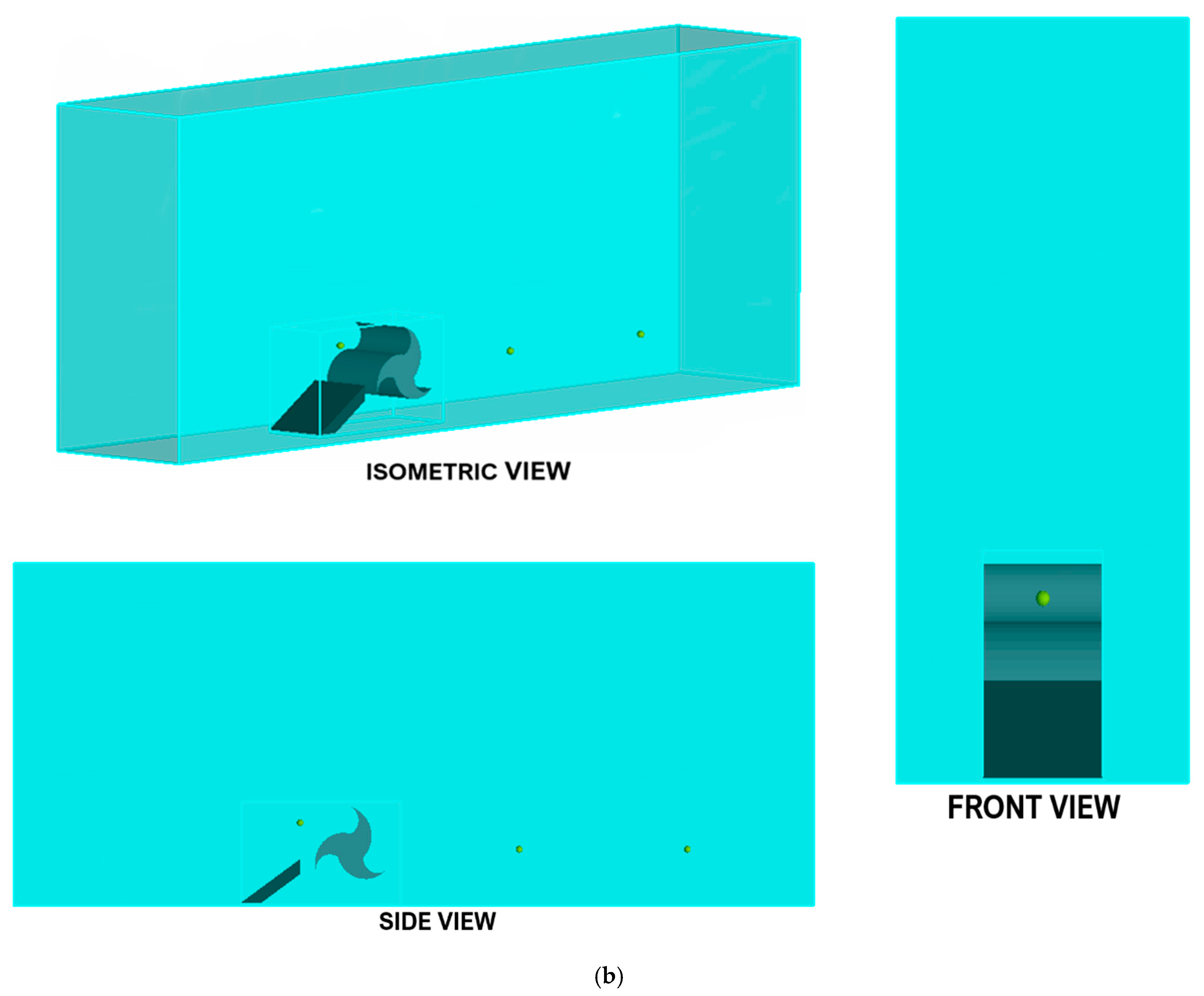
In the present study, the turbine design has been investigated for three different cases, as shown in Figure 2, and then comparisons have been made to exhibit the differences in the measured parameters. In the first case, the turbine has been analyzed without any deflectors, and for the second case, a deflector has been added to counter the negative torque on the returning blade. For the first two cases, the turbine is located in the vertical center of the computational domain. For the third case, the turbine with the deflector has been located at the base of the computational domain for studying the influence of a higher fluid pressure and proximity of the channel bed on the performance of the turbine. The initial study was carried out to determine the appropriate profile for the deflector plate. The flat profile for the deflector was chosen after measuring and comparing the torque values for both the curved and flat profiles at different angles for a specific Tip-Speed Ratio (TSR). Results for the same have been reported in Section 4. The numerical simulations have been carried out for a range of TSR, which vary from 0.6 to 1.8 at a flow velocity of 0.7 m/s. The computational fluid dynamics software Flow-3D has been used to run the numerical simulations and the turbine has been modeled in DesignModeler software. The standard k-epsilon (k-ε) turbulence model has been chosen for solving the Reynolds-Averaged Navier–Stokes equations (RANS) for the flow.

2. Theory and Governing Equations

2.1. CFD Model Description

The Finite Volume/Finite Differences Method (FVM/FDM) has been used to solve the governing Reynolds-Averaged Navier–Stokes equations (RANS) in a flow region which is subdivided into cartesian structured grid cells. The average values of every dependent variable are correlated with each cell. Every variable is located at the center of the cells except for velocity, which is located at the cell faces. The CFD software Flow-3D used for the current study employs the Volume of Fluid (VOF) method to solve the equations of motion in a turbulent flow. Flow-3D uses the Generalized Minimum Residual Method (GMRES) as the pressure–velocity solver. In this method, the pressure and velocity variables are coupled together implicitly through time-advanced pressures and time-advanced velocities in the momentum and continuity equations, respectively. This process of semi-implicitly formulating the finite-difference equations allows for an efficient solution in case of incompressible flow problems [33].
In Flow-3D, the equations to be solved are written in terms of cartesian co-ordinates x, y, and z representing the radial, azimuthal, and axial directions, respectively. The VOF method is based on a Eulerian fixed grid technique and was primarily introduced in 1981 by C.W. Hirt and B.D. Nichols [34]. It uses a fluid fraction scalar function ‘C’, which is defined as an integral of the characteristic function of the fluid volume in a computational grid cell. The value of the function ‘C’ always deviates between 0 to 1. As shown in Figure 3, when the mesh cell is empty with no fluid, the value of the C is 0, and is 1 when the fluid completely occupies the cell. It exhibits a discontinuous function 0 < C < 1 when there is some fluid interface in the cell but does not completely occupy the cell.
The governing equations for the three-dimensional incompressible flow analysis in Flow-3D are given as:
C ρ t + x ( u A x ) + y ( v A y ) + z ( w A z ) = R s o r ρ
where (u, v, w) are velocity components in the co-ordinate directions of (x, y, z); (Ax, Ay, Az) are the fractional areas in the given directions; density is given by ρ, and Rsor is a source term for density.
u t + 1 C ( u A x u x + v A y u y + w A z u z ) = 1 ρ p x + G x + f x
v t + 1 C ( u A x v x + v A y v y + w A v z ) = 1 ρ p y + G y + f y
w t + 1 C ( u A x w x + v A w y + w A w z ) = 1 ρ p z + G z + f z
where (Gx, Gy, Gz) represent the body accelerations in directions (x, y, z) and (fx, fy, fz) represent the viscous accelerations in co-ordinate directions (x, y, z) [33].

2.2. Standard k-ε Turbulence Model

The standard k-ε turbulence model with a no-slip wall shear boundary condition was used for the numerical simulations as it is preferred for high Reynolds number applications where the Reynolds shear stresses are important, such as in the case of this study, and as it has been widely used for similar studies [35]. A number of studies on the wind and ocean turbines have demonstrated acceptable agreement for the numerical results using a standard k-ε model with the experimental results. Sarma et al. [36] performed a numerical analysis on the Savonius hydrokinetic rotor using the k-ε turbulence model and validated it with the experimental results. The Cp value obtained was 0.39 from the experimental analysis and 0.402 from the numerical analysis showing an acceptable deviation of 1.03% between both the results. A study carried out by Doherty et al. [37] on a horizontal axis tidal turbine exhibited good agreement between the experimental and numerical values where the difference between the results was less than 2%. Similarly, some other studies have also achieved agreeable numerical results in comparison with the experimental values, thus showing the reliability of the standard k-ε model [38,39,40]. This turbulence model is also known as the two equation model as it uses two transport equations, namely, the equation for turbulent kinetic energy ‘k’, which determines the energy in the turbulence, and rate of dissipation of turbulence energy ‘ε’, which determines the scale of turbulence to solve the Reynolds stress tensor in the Reynolds-Averaged Navier–Stokes equations [41,42]. The equations used by the model have been explained below [43].
Turbulent kinetic energy (k):
t ( ρ k ) + x i ( ρ k u i ) = x j [ ( μ + μ t σ k ) k x j ] + P k + P b ρ ε Y M + S k
Dissipation rate (ε):
t ( ρ ε ) + x i ( ρ ε u i ) = x j [ ( μ + μ t σ ε ) ε x j ] + C 1 ε ε k ( P k + C 3 ε P b ) C 2 ε ρ ε 2 k + S ε
In the above two equations, Pk is the term for production of turbulent kinetic energy due to the gradient of mean velocity, Pb represents the turbulent kinetic energy due to the effect of buoyancy, YM is the contribution of fluctuating dilatation to the overall dissipation rate, xi is the co-ordinate in ith direction, µ is the dynamic viscosity, µt is turbulent dynamic viscosity, σk and σε represent the turbulent Prandtl numbers for k and ε, respectively, having a value of 1.39, terms C1ԑ, C2ԑ, and C3ԑ are the model constants. The turbulent viscosity (µt) is calculated using the equation:
μ t = ρ C μ k 2 ε
where C μ is a constant, having value of 0.09, which has been data fitted by numerous iterations for a wide range of turbulent flows according to [44].

2.3. Performance Equations

The power available for extraction for an OCT is given by the equation:
P a v a i l = 1 2 × ρ × A × v 3 .
The hydrodynamic performance characteristics studied in the present paper have been explained below:
Tip-speed ratio: It is a ratio of the speed of the tip of the blade to the incoming flow velocity and is represented as ‘λ’.
λ = ω × r v
Torque coefficient: It is the ratio of the total torque on the turbine to the total torque available in the flow and is represented as ‘Cm’.
C m = Q 0.5 × ρ × A s × v 2 × r
Power coefficient: It is the ratio of the power extracted by the turbine to the total available power in the flow and is represented as ‘Cp’.
C p =   Q × ω 0.5 × ρ × A s × v 3
The power coefficient can also be determined using the equation:
C p = C m × λ
In the above equations, ‘ω’ is the angular speed of turbine blades, ‘r’ is the turbine radius, ‘v’ is the flow velocity, ‘Q’ is the torque on the turbine blades, ‘ρ’ is the fluid density, and ‘As’ is the swept area of the turbine, which is taken as 0.665 (width times the diameter of the turbine).

3. Numerical Simulations Setup

3.1. Geometry Modelling and Computational Setup

The geometry of the turbine was created using DesignModeler software and then exported to Flow-3D for the numerical simulations. The turbine model investigated in the study was a horizontal axis three-bladed turbine having a diameter of 0.95 m. Figure 4 and Figure 5 show the dimensions of the turbine used for designing. The curved and flat deflector profiles and their dimensions compared have also been described. The inner and outer arc of each blade has a radius of 0.17 and 0.34 m, respectively. The smaller drum-like rotor connecting the three blades has a diameter of 0.35 m. The deflector in the front of the rotating blades has a thickness of 0.15 m. The angle of the deflector from the horizontal was determined to be 25° after comparing the torque values obtained at different angles at a fixed value of TSR. The width of the turbine blade is taken as 0.7 m. The turbine also has end plates of diameter 1.2 m and thickness 0.1 m, which act as a stationary supporting structure, but have been neglected for the present study considering the structure complexity and economy of computation time, and hence will be considered for future study. The modeled geometry was then converted to Stereolithography (STL) format and imported into Flow-3D. A rectangular computational domain has been used for the study. As shown in Figure 6, the inlet boundary is at a distance of 3.5D (D—diameter of turbine) upstream of the turbine so that a steady velocity state can develop at the location of the turbine and the outlet is at a distance of 4.5D downstream of the turbine. The side boundaries have been set to symmetry and are at a distance of 0.5 m on either side of the turbine. The bottom and the top boundaries are at a distance of 2D from the turbine center. The top boundary is set as specified pressure and the bottom boundary as wall in order for the hydrostatic pressure to build depending upon the depth of computational domain.
For the second and third cases, which involve the use of deflector, the deflector vane was specified as a solid stationary body. The turbine blades were set as a rotating body with a prescribed angular velocity required to assess the performance of the turbine at the required tip-speed ratio. The setup of Flow-3D accommodates the allocation of history probes at any required point in the domain, which records the output data at those selected points. In this case, three history probes—one just at the entrance point of the flow towards the turbine blades, the second at a distance of 2D downstream, and the third at a distance of 4D downstream—were specified as shown in the side view for Figure 6 to record the flow data at those respective points.
In Figure 6, the computational domain setup for Case 1 is not included as it has a similar arrangement as that for Case 2, the only difference being the absence of a deflector. Water was loaded as fluid and a fluid region was assigned in the entire computational domain. The standard k-ε turbulence model with no-slip as the wall shear boundary conditions was selected in the viscosity and turbulence section. Fluid pressure was activated in the fluid initial conditions and second order momentum advection was implemented for the simulations. The one fluid option with no sharp interface was selected from the general settings tab as the current study involves only one fluid and hence the free surface tracking algorithm was turned off. After implementing this setting, all open space in the mesh was filled by the selected single fluid at all times.

3.2. Meshing and Sensitivity Analysis

Flow-3D employs an orthogonal structured grid meshing method in terms of both the Cartesian and cylindrical co-ordinate systems. This allows the geometry and the mesh to be defined independently, meaning that the geometry can be modified without redefining the mesh. This makes the mesh generation simpler and faster as compared to the mesh generation for body fitted co-ordinates. The accuracy of the mesh in Flow-3D can be determined by using an in-built algorithm FAVOR (Fractional Area/Volume Obstacle Representation), which visualizes the geometry that will be interpreted by the solver for the simulation. The level of refinement required depends upon the FAVOR results, which can be reviewed before initiating the simulation. Upon achieving the desired accuracy in the FAVOR for a corresponding mesh cell size, the same mesh cell size can be adopted for the simulations. However, a smaller mesh size can be used to check if the further decrease in mesh size is leading to any considerable deviation in results or if the results are stable in comparison with the selected mesh cell size. A finer size of mesh helps the solver interpret the sharp curves in the geometry with better accuracy, but on the contrary, makes the solution tedious. However, different mesh planes can be added near the important sections in the computational domain and make the mesh finer, specifically for those regions to capture the near wall surface effects and balance the accuracy–time constraint ratio.
For this study, two non-conforming mesh blocks were used for meshing the computational domain with structured grids. Two different mesh blocks were used—the bigger mesh block with the outer boundaries of the computational domain and the smaller mesh block around the geometry for accurately capturing the forces on the turbine. The mesh sensitivity analysis was done by measuring the values of torque coefficient for different sizes of mesh cells. The mesh cell size was decreased for each analysis until a stable value was observed for any further reduction in the mesh cell size. The torque coefficient values for eight different levels of refinement are shown in Figure 7. The number of mesh cells corresponding to each refinement level is shown in Table 1.
The torque coefficient displays a stable value from the Refinement level 5 and hence the corresponding number of mesh cells, i.e., 9,878,000, were used for the study. The mesh cell size of 8 mm for the smaller mesh block enclosing the turbine geometry and 20 mm for the bigger mesh block was adopted to achieve the economy in computation time and was based on the FAVOR results obtained. Figure 8 shows the different results generated by the FAVOR algorithms based on the quality of mesh. The image on the left shows the geometry interpreted by the solver for Refinement level 1, while the image on the right shows the geometry interpreted for Refinement level 5. It is clear that a higher refinement level helps interpret the sharp curves and edges of the geometry. The turbulence models in Flow-3D use the logarithmic wall function for the cells intersecting a surface. It assumes the center of the cells is within the turbulent region of the logarithmic velocity profile. A y+ value of less than 300 is appropriate when a wall function is applied in the turbulence model [44]. The y+ values refer to the dimensionless distance between the wall to the first cell height. The wall function approach used in the current study requires this dimensionless distance to be greater than or equal to 30 [45] and hence a y+ value of 30 has been maintained in the present study.

4. Results and Discussion

4.1. Angle and Shape of Deflector

The use of a deflector for drag type turbines has shown considerable positive results as compared to bare turbines. The use of a deflector plate not only deflects the mass flux towards the approaching blade but also shields the returning blade, thus reducing the negative torque imposed by the flow on the returning blade. The flat deflector was selected for the turbine over the curved one after measuring the torque coefficients obtained for both the profiles. Initially, it was necessary to identify the optimum angle, which can generate the highest value of Cm for both the profiles. The angles were measured starting from 21° for both the profiles as at this value of angle the returning blade is almost shielded from the flow. The values of the angle were further increased by an interval of two degrees for each simulation until it reached 33°. From the torque coefficient values measured, it was observed that for every angle tested, the flat deflector profile gives a higher torque coefficient value than the corresponding value for the curved one. The flow streamlines when the advancing blade surface is completely exposed to the flow with both the flat and curved deflectors, as shown in Figure 9. The streamlines over the curved deflector seem to follow a slight vertically upward direction due to the curved profile of the deflector as compared to the streamlines over the flat deflector, which directs the flow into the exposed surface of the blade. It also explains why the flat profile gives a higher Cm as compared to the curved one and the reason why most of the studies considering the use of deflector for drag-based turbines have opted for flat deflector profiles over any other shape [46,47,48].
The values of Cm at all the deflector angles were measured for the same TSR value of 0.8, meaning at a fixed angular velocity, calculated using Equation (9), of the turbine and an inflow velocity of 0.7 m/s. Hence, based on the tangential velocity of the blade and the absolute inflow velocity, the velocity triangle analysis as shown in Figure 10 was implemented to obtain the relative flow velocity at the tip of the blade (Vr), the angle of the relative flow velocity (θ), and the angle made between the blade tip inclination and the relative flow velocity (β) for flow over both the flat and curved deflector. Relative velocity refers to the velocity of the incoming flow with respect to the turbine blade motion through which it flows. These parameters are important to determine the optimum configuration of the blade and deflector with respect to the incoming flow for subsequently minimizing the impact power losses on the turbine blades and increasing efficiency.
As shown in the Figure 10, the angle β was calculated at the blade tip section and the blade azimuthal position for this calculation was taken as 325°, as the turbine experiences high torque at this azimuthal angle. The absolute inflow velocity angle (α) is a very critical component for this calculation and needs to be specified with respect to the inclination of the flow approaching the blade tip. This angle was the same as the angle of the deflector for the flat deflector case, however, in the case of the curved deflector, the deflector curve surface follows a higher inclination towards the outflow edge. Hence, for the curved deflector, this angle was measured as the inclination of the tangent at the outflow edge of the deflector as shown in Figure 10 and is termed as ‘α’’. The different variables measured using the velocity triangle analysis for both the flat and curved deflector cases are given in Table 2.
In both the cases, the relative velocity increases with the increasing deflector angle. Although, for both the profiles, the highest value of Cm was measured at the deflector angle of 25°. For the flat deflector, the relative velocity at this angle was 0.304 m/s, while for the curved deflector inclined at 25°, the absolute inflow velocity angle was determined to be 37.32° and the relative velocity was 0.445 m/s. The highest achieved value of Cm for the curved deflector was 0.209 and for the flat deflector the highest value of Cm was 0.23. Another important observation, which can be derived from the analysis, is the optimum angle β that should be maintained between the blade tip inclination and the direction of relative flow velocity to minimize the impact power losses on the turbine blade. This optimum angle β for the curved and flat deflector was calculated to be 70.42° and 56.88°, respectively. These values were chosen as optimum as they corresponded to the maximum value of Cm obtained, thus indicating this flow orientation better matches with the blade profile. As the flat deflector gives the highest Cm value of the two profiles tested as shown in Figure 11, the same with an angle of 25° at the upstream of the turbine has been used in this study.

4.2. Measurements of Torque and Power Coefficients

The values for the torque and power coefficients have been calculated using the performance equations. The torque coefficients were obtained using Equation (10) for all the three cases and are shown in Figure 12. For Case 1, where the turbine was simulated without a deflector, the highest value of Cm achieved was 0.2 at a TSR of 0.8. Case 2 and 3 arrangements, where the turbine was provided with a deflector at different depths in the computational domain, reached a peak Cm of 0.237 and 0.19 at TSR values of 0.8 and 1.2, respectively. From the obtained results, it is clear that the turbine arrangement in the second case achieved the greater value of Cm at all the tip-speed ratios. The peak value of Cm for Case 2 was 18% and 24% higher than that achieved for Case 1 and 3, respectively. Another notable observation from this graph is that even though the peak value for turbine in Case 1 (0.2) was higher than Case 3 (0.19), a constantly higher stable value can be seen for the turbine with a deflector for most values of TSR.
The torque coefficient values obtained at the different azimuthal angles for the turbine in all the three cases are presented in Figure 13. These values were recorded when the flow velocity achieved a steady state. The turbine without a deflector in Case 1 experiences a negative torque in two ranges of operation: 120°–140° and 300°–320°. The value of negative torque reaches up to -0.04 at a 130° azimuthal angle and -0.03 at 310°. The occurrence of the negative torque values along some azimuthal angles is a common phenomenon, which depends upon the position of the blade at those respective angles, as well as differing for each type of turbine, and is also influenced by the number of blades. The angle of attack of the flow towards the azimuthal angle of the turbine also contributes to the positive or negative torque generation [49]. Examples of similar results, where the turbine experiences negative torque at some of the azimuthal angles, can be seen in [50,51,52] and many other studies. The higher values can be observed at 60°, 180°, 325°, and 360°.
Similarly, for Cases 2 and 3, the lowest values were observed for the same operation ranges as that for Case 1, but no negative torque was measured for these cases, thus exemplifying the advantages of the deflector to eliminate it. Higher values for Case 2 were measured at the angle of 20°, 325°, and 360°, while for Case 3, the peak values were obtained at 40°, 220°, and 360°.
The torques extracted in all the three cases at different rotating speeds expressed in Revolutions Per Minute (RPM) of the turbine are shown in Figure 14. The turbine without a deflector in Case 1 extracted the highest torque of 15.47 Nm at a rotating speed of 11.2 RPM. For Cases 2 and 3, the maximum extracted torques were 18.34 and 14.78 Nm at rotating speeds of 11.2 and 16.9 RPM, respectively. As the rotating speeds were further increased depending upon the tip-speed ratios, a decrease in the value of extracted torque can be observed from the graph, hence defining the optimum rotating speed of the different turbine arrangements for the given velocity.
The power coefficients achieved by the turbine for all the 3 cases are shown in Figure 15. These values were calculated using Equations (11) and (12). The first comparison can be made between Cases 1 and 2, where the turbine is operating at the same position along the vertical axis and the only modification being the use of a deflector for the second case. The maximum value of Cp obtained for Case 1 was 0.195 at a TSR value of 1. For Case 2, the turbine achieved a highest Cp value of 0.28 at a TSR of 1.2. From the equations used to calculate Cp, it is apparent that the efficiency of the turbine is directly dependent upon the torque coefficient values and hence the torque acting on the turbine. In Case 2, the deflector plate is acting as an obstacle to the flow and shielding the returning blade, thus preventing the generation of negative torque. This elimination of negative torque due to the use of a deflector is evident from Figure 13, which shows the torque coefficient over the entire azimuthal rotation of the turbine. In addition to covering the returning blade, the inclined profile of the deflector plate diverts the flow towards the exposed face of the advancing blade, thus increasing the mass flux approaching the turbine. Although the peak values for both the cases came at different TSRs, it clearly demonstrates the fact that a deflector provided in front of the turbine helps to achieve a higher value of Cp than that achieved for the bare turbine without a deflector.
Similarly, comparison can also be made between Cases 2 and 3 where the same arrangement of a turbine with a deflector operates at two different values of depth and pressure. Here, the value of the pressure at the respective operating location of the turbine is directly proportional to the depth of the operating location and increases with the depth. In Case 2, the turbine was located at a distance of 2D from the top boundary of the computational domain and the pressure at the location of the turbine was 1.813e+004 pascals. For Case 3, the location of the turbine is at a greater depth, which is 4D from the top boundary and hence a higher pressure acts on the turbine. The value of the pressure layer at the location of the turbine for Case 3 is 2.720e+004 pascals. As mentioned earlier, the maximum value of Cp for Case 2 is 0.28, while the turbine in Case 3 reached a crest Cp value of 0.23 at the same TSR of 1.2. The lower values of both Cp and Cm when the turbine is operating under higher hydrostatic pressure supports the fact that the maximum efficiency by an ocean current turbine is achieved when it is deployed at a lower depth from the free surface of the channel. On the other hand, the efficiency value deteriorates when the turbine is located at close proximity from the channel bed and is under a high hydrostatic pressure. A similar trend in results has been reported in some other studies focusing on the free surface effects and depth of deployment for the OCTs [53,54,55,56].

4.3. Hypothesis Testing

The torque and power coefficient data obtained from the simulations were subjected to hypothesis testing using statistical analysis. The paired t-test was adopted for the analysis. This statistical tool compares two sets of data to identify the differences within the data sets and determines the significant changes based on the null and alternative hypothesis. The conclusion for the paired t-test depends upon the obtained p-value after comparing the data sets. Generally, a 95% level of significance is considered for the paired t-test. The 95% level of significance indicates that if the achieved p-value is greater than 0.05 (5%), then in that case the null hypothesis is said to be true. However, if the p-value is smaller than 0.05, the alternative hypothesis is true. The closer the p-value is to zero, the stronger is the probability of the alternative hypothesis being true [57,58].
Four different cases, as shown in Table 3, were compared with each case comparing two data sets.
For each of the cases compared, the null hypothesis that there is no significant difference in the measured values was adopted. The alternative hypothesis indicated that both the data sets being compared differed significantly from each other. From the results of hypothesis testing, the p-values, mean, and standard deviation achieved for each of the data sets, and for the different comparisons of Cp and Cm, have been shown in Table 4, Table 5, Table 6 and Table 7.
The results achieved from the paired t-test for every compared case gave a p-value < 0.001. As this value was way below 0.05, the alternative hypothesis stating that each of the data sets compared differ significantly from each other can be said to be true. The distribution of differences for every case compared is shown in Figure 16. Furthermore, the location of mean value for each case can be observed.
From the statistical analysis, it is clear that for the Case A comparison, the turbine with a deflector achieves a maximum Cp value, which is 43% higher as compared to the maximum value of Cp for the turbine without a deflector in similar operating conditions. From the Case B comparisons, where the Cp values are compared for turbines operating at different depths, the turbine for Case 2 attains a Cp maximum value, which is 21% higher than that achieved for the turbine in Case 3. The difference in the peak values achieved for each of the cases, in which the value for Case 2 is the higher one, illustrates the influence of a greater pressure magnitude hampering the performance of the turbine. However, even at a greater fluid pressure, the Cp value measured for Case 3 was higher than that obtained for Case 1, which very well explains the advantage of deflector and its need to overcome the negative torque in drag types of hydrokinetic devices. A similar trend can be seen in terms of the torque coefficient for the comparisons made in Case C and Case D, where the turbine with a deflector at a lower operating depth (Case 2) gives better performance by 18% and 24% in each comparison, respectively.

5. Practical Applications

Most of the conventional hydrokinetic turbines are designed for locations having flow velocities greater than 1.2–1.5 m/s and for high ocean depths [59]. These limitations restrict their deployment for regions having shallow depths and low flow velocities. The studied design of the in-plane HAOCT can prove useful for such sites where the flow velocity is not feasible for deployment of the conventional designs and where the depth of the water channel is limited. In such a case, a number of rotors can be stacked side-by-side over a large distance across a channel flow to harness the kinetic energy. On the other hand, as mentioned earlier in Section 1, many optimization studies considering the use of a deflector, with some considering multiple deflectors, have been carried out for drag types of turbines. These studies, however, do not provide the overall turbine structure idea which can be practically installed in the water channels. For real applications, a design with structural equilibrium needs to be considered, rather than focusing on the sole purpose of achieving high efficiency, by proposing an unrealistic arrangement of deflectors. By taking into account the discussed design aspects for the current turbine design, a structural arrangement can be proposed where the rotor with the rotating blades and the deflector is connected to the end plates as shown in Figure 17.
These end plates can act as a stationary support structure, along with the deflector resting on the bed if the turbine is located at the channel bed for shallow water applications in the case of flat channel beds. For uneven channel beds, a foundation structure can be designed with the turbine structure attached to it by bolting, or any other suitable means. However, for deep water applications, a tethered system for a floating structure can be considered. From the overall analysis presented in this study, it can be stated that in order achieve the maximum performance, the turbine arrangement with a deflector oriented at 25° at the upstream of the blades operating at a TSR of 1.2 can harness power at an efficiency of 23% to 28%, depending upon the depth of operation, and in a flow velocity as low as 0.7 m/s.

6. Conclusions

The performance of a horizontal axis ocean current turbine was studied using three-dimensional numerical simulations, and comparisons were made for three different cases of operation. The achieved results exhibit that the Case 2 arrangement, where the turbine with a deflector was located at the center of the computational domain, achieved higher power and torque coefficients (0.28 and 0.237) in comparison to the turbine without a deflector (0.195 and 0.195) and the turbine with a deflector at a higher depth (0.23 and 0.191). The torque coefficients at different azimuthal angles along the 360° rotation of the turbine were measured, and a distinguishable outcome from the results can be observed for the turbine without a deflector where a negative torque was induced for two different operating ranges (120°–140° and 300°–320°). There were no negative values when the turbine was simulated with a deflector for the other two cases, which highlights the enhancement of turbine performance due to the use of a deflector. From the context of operating depth, it can be concluded that the given turbine demonstrates better performance when it is operating under low hydrostatic pressure conditions. On the contrary, the efficiency of the turbine was seen to deteriorate when it was operating under comparatively higher hydrostatic pressure and in close proximity to the tank bed. For shallow waters, however, the turbine with a deflector and stationary end plates can also be installed on the seabed. The values of power coefficients can be said to be very much acceptable given the low flow velocity of 0.7 m/s in which the turbine was simulated.

7. Future Work

The future work will consider varying the radius of the inner and outer arcs of the turbine blade and determining the optimum radius values which can generate the maximum torque. The concept of velocity triangle will be used for determining the optimum deflector angle in future modifications of the design using flow-driven simulations on the turbine. The present study only considered the blade and deflector, and hence future work will include the end plates at the either end of the blade. From a number of studies, the use of end plates has shown considerable improvement in the performance of Savonius turbine design, and as the current design operates on a similar drag mechanism, an increase in efficiency of the device with the integration of end plates can be expected. Likewise, the optimum aspect ratio for the turbine, which is the ratio of the width to the diameter of the turbine, will be investigated. The parameter of aspect ratio can be useful for commercial manufacturing of large-scale devices for practical applications.

Author Contributions

This study was designed by C.Y.N. The numerical analysis and manuscript writing were performed by N.R.M. under the supervision of C.Y.N., L.W.E., and E.O. The reviewing and editing were done by A.F. and H.S.K. All authors have read and agree to the published version of the manuscript.

Funding

This research was funded by Yayasan UTP grant Cost centre: 0153AA-E37.

Acknowledgments

The authors would like to acknowledge financial support from Universiti Teknologi PETRONAS, YUTP grant (Cost centre: 0153AA-E37). Also, the authors would like to acknowledge Mohd Shahir Liew, Universiti Teknologi Petronas for his support and encouragement towards this research. Nevertheless, the authors would like to acknowledge management of Universiti Teknologi PETRONAS, Middle East Technical University, Universiti Tenaga Nasional, Universiti Malaya Terengganu and Universiti Teknologi Malaysia for the continuous support and encouragement.

Conflicts of Interest

The authors declare no conflict of interest.

References

  1. Wellmann, J.; Morosuk, T. Renewable energy supply and demand for the city of El Gouna, Egypt. Sustainability 2016, 8, 314. [Google Scholar] [CrossRef] [Green Version]
  2. Karim, M.E.; Karim, R.; Islam, M.T.; Muhammad-Sukki, F.; Bani, N.A.; Muhtazaruddin, M.N. Renewable energy for sustainable growth and development: An evaluation of law and policy of Bangladesh. Sustainability 2019, 11, 5774. [Google Scholar] [CrossRef] [Green Version]
  3. Oğuz, E.; Şentürk, A.E. Selection of the most sustainable renewable energy system for Bozcaada Island: Wind vs. Photovoltaic. Sustainability 2019, 11, 4098. [Google Scholar] [CrossRef] [Green Version]
  4. Tareen, W.U.; Dilbar, M.T.; Farhan, M.; Nawaz, M.A.; Durrani, A.W.; Memon, K.A.; Mekhilef, S.; Seyedmahmoudian, M.; Horan, B.; Amir, M.; et al. Present Status and Potential of Biomass Energy in Pakistan Based on Existing and Future Renewable Resources. Sustainability 2020, 12, 249. [Google Scholar] [CrossRef] [Green Version]
  5. Arroyo, M.; Flavio, R.; Miguel, L.J. The Trends of the Energy Intensity and CO 2 Emissions Related to Final Energy Consumption in Ecuador: Scenarios of National and Worldwide Strategies. Sustainability 2020, 12, 20. [Google Scholar] [CrossRef] [Green Version]
  6. Bedard, R.; Jacobson, P.T.; Previsic, M.; Musial, W.; Varley, R. An overview of ocean renewable energy technologies. Oceanography 2010, 23, 22–31. [Google Scholar] [CrossRef]
  7. Nachtane, H.B.M.; Tarfaoui, M.; Moumen, A.; Saifaoui, D. Design and Hydrodynamic Performance of a Horizontal Axis Hydrokinetic Turbine. Int. J. Automot. Mech. Eng. 2019, 16, 6453–6469. [Google Scholar]
  8. Lestari, H.; Arentsen, M.; Bressers, H.; Gunawan, B.; Iskandar, J. Sustainability of renewable off-grid technology for rural electrification: A comparative study using the IAD framework. Sustainability 2018, 10, 4512. [Google Scholar] [CrossRef] [Green Version]
  9. Liang, X.; Si, D.; Xu, J. Quantitative evaluation of the sustainable development capacity of hydropower in China based on information entropy. Sustainability 2018, 10, 529. [Google Scholar] [CrossRef] [Green Version]
  10. Ehrbar, D.; Schmocker, L.; Vetsch, D.F.; Boes, R.M. Hydropower potential in the periglacial environment of Switzerland under climate change. Sustainability 2018, 10, 2794. [Google Scholar] [CrossRef] [Green Version]
  11. Magagna, D.; Uihlein, A. Ocean energy development in Europe: Current status and future perspectives. Int. J. Mar. Energy 2015, 11, 84–104. [Google Scholar] [CrossRef]
  12. Le Traon, P.Y.; Morrow, R. Ocean currents and eddies. Int. Geophys 2001, 69, 171–215, ix–xi. [Google Scholar]
  13. Hu, S.; Sprintall, J.; Guan, C.; McPhaden, M.J.; Wang, F.; Hu, D.; Cai, W. Deep-reaching acceleration of global mean ocean circulation over the past two decades. Sci. Adv. 2020, 6, 1–9. [Google Scholar] [CrossRef] [PubMed] [Green Version]
  14. White, I.L.; Kash, D.E. Energy under the Oceans: A Technology Assessment of Outer Continental Shelf Oil and Gas Operations; The University of Oklahoma Press: Noman, OK, USA, 1973. [Google Scholar]
  15. Mayor, B.; Rodríguez-Muñoz, I.; Villarroya, F.; Montero, E.; López-Gunn, E. The role of large and small scale hydropower for energy and water security in the Spanish Duero basin. Sustainability 2017, 9, 1807. [Google Scholar] [CrossRef] [Green Version]
  16. Laws, N.D.; Epps, B.P. Hydrokinetic energy conversion: Technology, research, and outlook. Renew. Sustain. Energy Rev. 2016, 57, 1245–1259. [Google Scholar] [CrossRef] [Green Version]
  17. Fraenkel, P.L. Marine current turbines: Pioneering the development of marine kinetic energy converters. Proc. Inst. Mech. Eng. Part A J. Power Energy 2007, 221, 159–169. [Google Scholar] [CrossRef]
  18. Tian, W.; Mao, Z.; Ding, H. Design, test and numerical simulation of a low-speed horizontal axis hydrokinetic turbine. Int. J. Nav. Archit. Ocean Eng. 2018, 10, 782–793. [Google Scholar] [CrossRef]
  19. Mukherji, S. Design and Critical Performance Evaluation of Horizontal Axis Hydrokinetic Turbines. Master’s Thesis, Missouri University of Science and Technology, Rolla, MO, USA, 2010. [Google Scholar]
  20. Yaakob, O.B.; Tawi, K.B.; Sunanto, D.T.S. Computer simulation studies on the effect overlap ratio for savonius type vertical axis marine current turbine. Int. J. Eng. Trans. A Basics 2010, 23, 79–88. [Google Scholar]
  21. Osbourne, N.; Groulx, D.; Penesis, I. Three dimensional simulation of a horizontal axis tidal turbine comparison with experimental results. In Proceedings of the 2nd Asian Wave and Tidal Energy Conference, Tokyo, Japan, 27–30 July 2014. [Google Scholar]
  22. Bai, X.; Avital, E.J.; Williams, J.J.R. Numerical Simulation of A Marine Current Turbine in Turbulent Flow. Ph.D. Thesis, Queen Mary University of London, London, UK, 2014; pp. 1–7. [Google Scholar]
  23. Khan, M.J.; Bhuyan, G.; Iqbal, M.T.; Quaicoe, J.E. Hydrokinetic energy conversion systems and assessment of horizontal and vertical axis turbines for river and tidal applications: A technology status review. Appl. Energy 2009, 86, 1823–1835. [Google Scholar] [CrossRef]
  24. Khan, M.J.; Iqbal, M.T.; Quaicoe, J.E. River current energy conversion systems: Progress, prospects and challenges. Renew. Sustain. Energy Rev. 2008, 12, 2177–2193. [Google Scholar] [CrossRef]
  25. Asterita, T.J. Available online: www.waterotor.com (accessed on 8 October 2019).
  26. Golecha, K.; Eldho, T.I.; Prabhu, S.V. Influence of the deflector plate on the performance of modified Savonius water turbine. Appl. Energy 2011, 88, 3207–3217. [Google Scholar] [CrossRef]
  27. Sahim, K.; Ihtisan, K.; Santoso, D.; Sipahutar, R. Experimental Study of Darrieus-Savonius Water Turbine with Deflector: Effect of Deflector on the Performance. Int. J. Rotating Mach. 2014, 14, 1–6. [Google Scholar] [CrossRef] [Green Version]
  28. Akinyemi, O.S.; Liu, Y. CFD modeling and simulation of a hydropower system in generating clean electricity from water flow. Int. J. Energy Environ. Eng. 2015, 6, 357–366. [Google Scholar] [CrossRef] [Green Version]
  29. Quaranta, E. Stream water wheels as renewable energy supply in flowing water: Theoretical considerations, performance assessment and design recommendations. Energy Sustain. Dev. 2018, 45, 96–109. [Google Scholar] [CrossRef]
  30. Hemida, M.; Ramadan, A.; Aissa, W.A. Numerical Investigation of Hydrokinetic Savonius Rotor with Two Shielding Plates. Appl. Model. Simul. 2019, 3, 85–94. [Google Scholar]
  31. Kolekar, N.; Banerjee, A. Performance characterization and placement of a marine hydrokinetic turbine in a tidal channel under boundary proximity and blockage effects. Appl. Energy 2015, 148, 121–133. [Google Scholar] [CrossRef]
  32. Welander, P. A discussion on ocean currents and their dynamics-The thermocline problem. Philos. Trans. R. Soc. A 1971, 270, 415–421. [Google Scholar]
  33. FLOW-3D User Manual v11.2; Flow Science, Inc.: Santa Fe, NM, USA, 2008; p. 300.
  34. Hirt, C.W. Volume of Fluid (VOF) Method for the Dynamics of Free Boundaries *. J. Comput. Phys. 1981, 225, 201–225. [Google Scholar] [CrossRef]
  35. Launder, B. The numerical computation of turbulent flows. In Numerical Prediction of Flow, Heat Transfer, Turbulence and Combustion; Elsevier: Pergamon, Turkey, 2017. [Google Scholar]
  36. Sarma, N.K.; Biswas, A.; Misra, R.D. Experimental and computational evaluation of Savonius hydrokinetic turbine for low velocity condition with comparison to Savonius wind turbine at the same input power. ENERGY Convers. Manag. 2014, 83, 88–98. [Google Scholar] [CrossRef]
  37. O’Doherty, T.; Mason-Jones, A.; O’Doherty, D.M.; Byrne, C.B.; Owen, I.; Wang, Y.X. Experimental and Computational Analysis of a Model Horizontal Axis Tidal Turbine. In Proceedings of the 8th European Wave and Tidal Energy Conference, Uppsala, Sweden, 7–10 September 2009; pp. 833–841. [Google Scholar]
  38. Wahyudi, B.; Adiwidodo, S. The influence of moving deflector angle to positive torque on the hydrokinetic cross flow savonius vertical axis turbine. Int. Energy J. 2017, 17, 11–21. [Google Scholar]
  39. Yaakob, O.; Ahmed, Y.; Ismail, M. Validation study for savonius vertical axis marine current turbine using CFD simulation. In Proceedings of the 6th Asia-Pacific Workshop on Marine Hydrodynamics-APHydro, Johor Bahru, Malaysia, 3–4 September 2012. [Google Scholar]
  40. Mohamed, M.H.; Janiga, G.; Pap, E.; Thévenin, D. Optimal blade shape of a modified Savonius turbine using an obstacle shielding the returning blade. Energy Convers. Manag. 2011, 52, 236–242. [Google Scholar] [CrossRef]
  41. Soe, T.M.; Khaing, S.Y. Comparison of Turbulence Models for Computational Fluid Dynamics Simulation of Wind Flow on Cluster of Buildings in Mandalay. Int. J. Sci. Res. Publ. 2017, 7, 337–350. [Google Scholar]
  42. Rusdin, A. Computation of turbulent flow around a square block with standard and modified k-ε turbulence models. Int. J. Automot. Mech. Eng. 2017, 14, 3938–3953. [Google Scholar] [CrossRef]
  43. Recktenwald, G.; Turbulence, W.I. The k–ε Turbulence Model. ME 2009, 448, 548. [Google Scholar]
  44. Ruffin, S.M.; Lee, J. Adaptation of a k-epsilon Model to a Cartesian Grid Based Methodology. Int. J. Math. Models Methods Appl. Sci. 2009, 3, 238–245. [Google Scholar]
  45. Rahimian, M.; Walker, J.; Penesis, I. Numerical assessment of a horizontal axis marine current turbine performance. Int. J. Mar. Energy 2017, 20, 151–164. [Google Scholar] [CrossRef]
  46. Yaakob, O.; Ismail, M.A.; Ahmed, Y.M. Parametric Study for Savonius Vertical Axis Marine Current Turbine using CFD Simulation 2 Literature Review. In Proceedings of the 7th International Conference on Renewable Energy Sources (RES’13), Kuala Lumpur, Malaysia, 2–4 April 2013; pp. 200–205. [Google Scholar]
  47. Kailash, G.; Eldho, T.I.; Prabhu, S.V. Performance study of modified savonius water turbine with two deflector plates. Int. J. Rotating Mach. 2012, 12, 1–12. [Google Scholar] [CrossRef] [Green Version]
  48. Kaprawi, S.; Santoso, D.; Sipahutar, R. Performance of combined water turbine darrieus-savonius with two stage savonius buckets and single deflector. Int. J. Renew. Energy Res. 2015, 5, 217–221. [Google Scholar]
  49. Batten, W.M.J.; Bahaj, A.S.; Molland, A.F.; Chaplin, J.R. Hydrodynamics of marine current turbines. Renew. Energy 2006, 31, 249–256. [Google Scholar] [CrossRef] [Green Version]
  50. Satrio, D.; Aria, I.K.; Utama, P. Numerical Investigation of Contra Rotating Vertical-Axis Tidal-Current Turbine. J. Mar. Sci. Appl. 2018, 17, 208–215. [Google Scholar] [CrossRef]
  51. Liu, Z.; Wang, Z.; Shi, H.; Qu, H. Numerical Study of a Guide-Vane-Augmented Vertical Darrieus. J. Hydrodyn. 2018, 31, 522–530. [Google Scholar] [CrossRef]
  52. Sumantraa, B.; Santhanam, C. Numerical Analysis of Effect of Pitch Angle on a Small Scale Vertical Axis Wind Turbine. Int. J. Renew. Energy Res. 2014, 4, 929–935. [Google Scholar]
  53. Birjandi, A.H.; Bibeau, E.L.; Chatoorgoon, V.; Kumar, A. Power measurement of hydrokinetic turbines with free-surface and blockage effect. Ocean Eng. 2013, 69, 9–17. [Google Scholar] [CrossRef]
  54. Garrett, C.; Cummins, P. The efficiency of a turbine in a tidal channel. J. Fluid Mech. 2007, 588, 243–251. [Google Scholar] [CrossRef] [Green Version]
  55. Bai, X.; Avital, E.J.; Munjiza, A.; Williams, J.J.R. Numerical simulation of a marine current turbine in free surface flow. Renew. Energy 2014, 63, 715–723. [Google Scholar] [CrossRef]
  56. Zhou, J.W.; Wang, D.Z. Simulation of tidal stream turbine working near free surface. Appl. Mech. Mater. 2013, 363, 291–295. [Google Scholar] [CrossRef]
  57. Mccluskey, A.; Lalkhen, A.G. Statistics IV: Interpreting the results of statistical tests. Contin. Educ. Anaesth. Crit. Care Pain 2007, 7, 208–212. [Google Scholar] [CrossRef] [Green Version]
  58. Xu, M.; Fralick, D.; Zheng, J.Z.; Wang, B.; Tu, X.M.; Feng, C. The differences and similarities between two-sample t-test and paired t-test. Shanghai Arch. Psychiatry 2017, 29, 184–188. [Google Scholar]
  59. Omar, Y.; Tengku, T.; Mohamad, A. Prospects for ocean energy in Malaysia. In Proceedings of the International Conference on Energy and Environment (ICEE), Selangor, Malaysia, 28–30 August 2006; pp. 63–68. [Google Scholar]
Figure 1. Turbine blade concept.
Sustainability 12 03333 g001
Figure 2. (a) Turbine arrangement for Case 1; (b) turbine arrangement for Case 2; (c) turbine arrangement for Case 3.
Sustainability 12 03333 g002
Figure 3. Fluid volume fraction representation.
Sustainability 12 03333 g003
Figure 4. Modeled geometry 2D sketch.
Sustainability 12 03333 g004
Figure 5. Modeled geometry isometric view.
Sustainability 12 03333 g005
Figure 6. (a) Computational domain for Case 2; (b) computational domain for Case 3.
Sustainability 12 03333 g006aSustainability 12 03333 g006b
Figure 7. Torque coefficient vs. mesh refinement levels.
Sustainability 12 03333 g007
Figure 8. (a) Geometry interpreted for Refinement level 1; (b) geometry interpreted for Refinement level 5.
Sustainability 12 03333 g008
Figure 9. (a) Flow streamlines for a flat deflector; (b) flow streamlines for a curved deflector.
Sustainability 12 03333 g009
Figure 10. Velocity triangle for the turbine blade.
Sustainability 12 03333 g010
Figure 11. Angle of deflector vs. torque coefficient.
Sustainability 12 03333 g011
Figure 12. Tip-speed ratio vs. torque coefficient.
Sustainability 12 03333 g012
Figure 13. Azimuthal angle vs. torque coefficient.
Sustainability 12 03333 g013
Figure 14. Rotating speed vs. torque.
Sustainability 12 03333 g014
Figure 15. Tip-speed ratio vs. power coefficient.
Sustainability 12 03333 g015
Figure 16. Distribution of differences: (a) for Case A; (b) for Case B; (c) for Case C; (d) for Case D.
Sustainability 12 03333 g016
Figure 17. Turbine structural arrangement.
Sustainability 12 03333 g017
Table 1. Number of mesh cells for different refinement levels.
Refinement LevelNo. of Mesh CellsMesh Cell Size (mm)
Bigger Mesh BlockSmaller Mesh Block
11,009,4004020
21,6634243417
33,120,9322813
45,958,2402310
59,878,000208
618,671,088176
746,699,438144
8257,178,582122
Table 2. Velocity triangle components.
Flat DeflectorCurved Deflector
α°θ°Vr (m/s)β°α′°θ°Vr (m/s)β°
2169.590.26650.5633.2986.980.38067.95
2373.490.28054.4635.5288.730.40669.70
2575.910.30456.8837.3289.450.42470.42
2778.750.32359.7239.6487.300.44568.27
2981.270.34262.2441.8385.210.46766.18
3183.650.36264.6243.6383.600.48564.57
3385.930.38066.9045.6881.800.50562.77
Table 3. Different cases for hypothesis testing.
Case AComparison of Cp values obtained for Case 1 and Case 2 turbine arrangements
Case BComparison of Cp values obtained for Case 2 and Case 3 turbine arrangements
Case CComparison of Cm values obtained for Case 1 and Case 2 turbine arrangements
Case DComparison of Cm values obtained for Case 2 and Case 3 turbine arrangements
Table 4. Paired t-test for power coefficient data.
CaseCase 1 Case 2 Hypothesis Testing Paired t-Test
meanStandard DeviationmeanStandard DeviationmeanStandard Deviationp-value
A0.1310.0480.1890.056−0.0570.233<0.001
Table 5. Paired t-test for power coefficient data.
CaseCase 2 Case 3 Hypothesis Testing Paired t-Test
meanStandard DeviationmeanStandard DeviationmeanStandard Deviationp-value
B0.1890.0560.14860.0480.0400.009<0.001
Table 6. Paired t-test for torque coefficient data.
CaseCase 1 Case 2 Hypothesis Testing Paired t-Test
meanStandard DeviationmeanStandard DeviationmeanStandard Deviationp-value
C0.1260.0610.1750.068−0.0480.017<0.001
Table 7. Paired t-test for torque coefficient data.
CaseCase 2 Case 3 Hypothesis Testing Paired t-Test
meanStandard DeviationmeanStandard DeviationmeanStandard Deviationp-value
D0.1750.0680.1370.0530.0370.015<0.001

