Minutely Active Power Forecasting Models Using Neural Networks

Abstract

Power forecasting is an integral part of the Demand Response design philosophy for power systems, enabling utility companies to understand the electricity consumption patterns of their customers and adjust price signals accordingly, in order to handle load demand more effectively. Since there is an increasing interest in real-time automation and more flexible Demand Response programs that monitor changes in the residential load profiles and reflect them according to changes in energy pricing schemes, high granularity time series forecasting is at the forefront of energy and artificial intelligence research, aimed at developing machine learning models that can produce accurate time series predictions. In this study we compared the baseline performance and structure of different types of neural networks on residential energy data by formulating a suitable supervised learning problem, based on real world data. After training and testing long short-term memory (LSTM) network variants, a convolutional neural network (CNN), and a multi-layer perceptron (MLP), we observed that the latter performed better on the given problem, yielding the lowest mean absolute error and achieving the fastest training time.

1. Introduction

The evolution of the smart grid and smart metering technology has enabled electricity providers to develop more sophisticated Demand Response (DR) programs in order to influence the consumption patterns of their customers by adjusting pricing signals. In the modern grid, Demand Response programs exploit the dependencies of the information streams that flow between customers and suppliers. Customers allow for their load profiles to be created and scrutinized, by providing smart meter data that reflect their consumption patterns; the data are derived simply from the daily operation of their devices. Suppliers are then able to interpret that data, and after identifying the demand trends, they can reflect them on supply expectations via price signal alterations that, in turn, can shift or change consumption patterns. In this way, electricity demand may be handled in a dynamic environment. In search of greater Demand Response flexibility and optimization as well as better third-party support through automation there is a lot of ongoing research in the field that is focused on the development of more precise load forecasting techniques, in order to obtain even more dynamic price signal adjustments. Hence, there is a considerable contribution from the areas of artificial intelligence and machine learning to the energy sector by way of various models and techniques aimed at managing and predicting real-time price and load fluctuations [1].

Since the data extracted from smart meters is in the form of time series, many statistical methods and classical machine learning models have relatively difficult implementations due to the temporal difference of the data points and the limitations concerning missing values, data dependencies, and dimensionality. The problem of missing values refers to the complete absence of some samples or the existence of non-interpretable data entries in a dataset [2]. Missing values introduce a level of uncertainty and bias which degrades the performance of classical models. Therefore, the reasons behind the existence of missing data need to be identified and imputation techniques in the preprocessing of the data have to be considered in order to create more robust classical models. On the other side of the spectrum, neural network models often omit missing values without a significant loss of quality in the results. Furthermore, data dependencies refer to the hidden relationships and patterns, such as trends, which could provide useful insights about the time series [3]. Traditional Autoregressive Integrated Moving Average (ARIMA) models are based on linear relationships and not on the joint distribution of random variables. Hence, nonlinear trends are not fully explored. Additionally, the limitation of dimensionality refers to the ability of the model to process a large number of input variables derived from different time series efficiently, while yielding meaningful results [4]. Traditional models focus primarily on univariate input data, considerably limiting the potential insights derived from richer time series datasets [5]. Neural networks are more suitable for handling complex relationships within the data and for developing robust forecasting models that are tolerant to noise: long short-term memory (LSTM) networks [6] are capable of identifying the long-term dependencies between data points and convolutional neural networks (CNNs) [7] can extract features from the raw input sequence and encode them in a low-dimensional space. The multi-layer perceptron (MLP) [8] can model non-linear trends and is able to handle missing values in the datasets well.

In 2015, Alamaniotis and Tsoukalas [9] presented a data-driven method for minutely active power forecasting based on Gaussian processes. This research project highlighted the importance of minute predictions in the residential setting due to the volatile nature of household consumption and examined machine learning models that outperformed the more traditional autoregressive moving average approach. In 2017, Singh et al. [10] trained an artificial neural network comprising 20 neurons in order to conduct short-term load forecasting of the NEPOOL region of ISO New England and yielded a decent Mean Absolute Percentage Error (M.A.P.E) performance while training on weekday data points. In 2018, Kuo and Huang [11] proposed the Deep Energy neural network structure, which consisted of an input layer, a feature extraction module, and a forecasting module. The tuning of the parameters in the convolution layers of the feature extraction module and the data flattening layer in the forecasting module resulted in relatively high precision short-term load predictions. Hossen et al. [12] examined deep neural network architectures in order to accurately forecast residential load consumption for a single user with one-minute resolution based on one year of historical data sets. Zhang et al. [13] reviewed machine learning methods in smart grids and outlined state-of-the-art approaches in the field of load forecasting. Kampelis et al. [14] used the genetic algorithms and neural networks to evaluate day-ahead load shifting techniques. Koponen et al. [15] presented physical- and data-driven models for Demand Response. Their work presented a very useful comparison of a support vector machine and a multi-layer perceptron for power forecasting. In a more recent work, Ahmad et al. [16] proposed a modular neural network model for load forecasting which consisted of a pre-processing module for the input time series, a forecast module where the artificial neural networks were trained, and an optimization module which helped minimize the forecast error. Walther et al. [17] utilized machine learning processing techniques such as feature engineering and hyperparameter tuning in order to optimize a Gradient Boosting Regression Trees (GBRT) algorithm which performs very short-term load forecasts with a 15-minute horizon based on minutely sampled data. Zhu et al. [18] presented a comparative study of deep learning techniques using minute-level real-world data of a plug-in electric vehicle charging station in order to evaluate the performance of those approaches on a variety of timesteps. The results of this study are valuable to machine learning researchers in the energy sector due to the examination of many different configurations in the deep learning space. Gasparin et al. [19] assessed the performance of deep recurrent neural networks on minutely sampled datasets of individual household electric power consumption in order to pave the way for standardized evaluation of the most optimal forecasting solutions in the field. Susan Li [20], in an article about time series prediction using LSTM, highlighted the minutely sampled data of a residential dataset provided by the University of California at Irvine (UCI). Cheekoty [21] presented the main advantages of neural network techniques over classical machine learning in time series forecasting, and, finally, Orac [22] constructed an LSTM model in order to predict trading data.

In this study, we focus on the minutely active power forecasting for residential electricity consumption, since we believe that, despite their overall complexity, accurate high granularity models can lead to fine-grained price signal adjustments. In the development of those models we use the types of neural networks mentioned above on the individual household electric power consumption data set found in the UCI machine learning repository [23]. The main purpose of this work is to compare the baseline performance of each network on the same dataset and provide useful remarks on the training process of each model. There is little work in the area of minute power forecasting and our study is the first concise comparison of the core neural network types on this prediction horizon with experiments conducted on residential active power data. In Section 2, we explain the methodology and the concepts that were followed to conduct the experiments. In Section 3 we present the results of our experiments through evaluation metrics relevant to the training process and the prediction quality of each network. Finally, in Section 4 we discuss the results obtained and suggest some directions for future work.

2. Materials and Methods

2.1. Neural Networks and Performance Metrics

In this subsection it is important to provide a concise introduction to the neural networks and the performance metrics we used for our experiments in order to outline their primary behavior prior to presenting the configurations of our machine learning models.

2.1.1. Multi-Layer Perceptron

The multi-layer perceptron extends the perceptron learning algorithm [24] and uses neurons arranged in layers in order to form a feedforward artificial neural network that approximates a function. This type of neural network uses a non-linear transformation on the input, which is learnt through the adjustment of weights and biases in the intermediate layers of the network. For simplicity, we considered a multi-layer perceptron with one hidden layer. This MLP approximated a function $f:R^D\to R^L$, where $D$ is the size of the input vector $x$ and $L$ is the size of the output vector $f\left(x\right)$. Following the matrix notation, the MLP, which consisted of an input layer, a hidden layer, and an output layer, can be expressed by the following formula:

$$f\left(x\right)=G\left(b^{\left(2\right)}+W^{\left(2\right)}\left(s(b^{\left(1\right)}+W^{\left(1\right)}x)\right)\right),$$

(1)

where $b^{\left(1\right)}$ and $W^{\left(1\right)}$ are the bias vector and weight matrix from the input vector to the hidden layer, $b^{\left(2\right)}$ and $W^{\left(2\right)}$ constitute the bias vector and weight matrix from the hidden layer to the output. Activation functions $s$ and $G$ define the output of the hidden layer and the output layer, respectively, given a set of inputs. The MLP was trained through backpropagation in order to minimize the error in the output, while approaching the expected result. The change in each weight was calculated with gradient descent [25].

2.1.2. Convolutional Neural Network

Convolutional neural networks share the same principles as other artificial neural networks, such as MLP, since they also consist of neurons arranged in layers and utilize iterative weight and bias updates to learn a function. The main differences with other types of neural networks lie in the operations performed, the architecture, and the areas of application. Convolutional neural networks perform kernel convolution by passing matrices of numbers, the kernels or filters, over the input in order to detect features. The base architecture of a CNN consists of the convolutional layer, the pooling layer, and the fully connected layer. The convolutional layer performs the kernel operation described above in order to produce a feature map. Pooling layers use the sliding window method in order to downsample the feature map, reducing its dimensions. The inclusion of pooling layers helps the networks train faster and provides an extra layer of safety against overfitting. Since convolution and pooling layers follow a 3D arrangement of neurons, data need to be flattened in order to produce 1D vectors in the output. Furthermore, fully connected layers are used on flattened input in order to produce the output of the CNN model. Figure 1 illustrates the structure of a convolutional neural network. The training process of CNNs shares the same concepts as MLPs but the formulas used throughout this process are modified to accommodate the differences in neuron arrangement and the usage of convolution. This type of neural network is particularly popular in image recognition, since image data can be segmented appropriately [26]. For the purposes of our study, we conducted some experiments on the 1D CNN, since this variant handles data with low dimensionality and is suitable for time series and sensor data analysis.

2.1.3. Long Short-Term Memory Network

Long short-term memory networks constitute a variation of recurrent neural networks (RNN) [28] primarily designed to handle long-term data dependencies. Similar to RNN, the LSTM follows a structure consisting of blocks, the LSTM cells. Each cell has its own state $C_t$, which is passed down to all the blocks in the network. Since the cell state passes through all the LSTM cells, each cell can adjust the state by removing or adding information. Information flowing through the cell state can be regulated with the forget, input, and output gates of every cell. The forget gate of a cell at the timestamp $t$ helps with information removal and can be expressed with the following formula:

$$f_t=\sigma \left(w_f\left[h_{t-1},x_t\right]+b_f\right),$$

(2)

where $x_t$ is the information at the current timestamp, $h_{t-1}$ is the output of the previous LSTM block, $w_f$ is the weight of the gate, $b_f$ is the bias, and $\sigma$ is the sigmoid function. Similarly, in Equations (3) and (4) the input and output gate are expressed with $b_i$ and $b_o$ being the respective biases and $w_i$ and $w_o$ the respective weights.

$$i_t=\sigma \left(w_i\left[h_{t-1},x_t\right]+b_i\right)$$

(3)

$$o_t=\sigma \left(w_o\left[h_{t-1},x_t\right]+b_o\right)$$

(4)

The input gate indicates which values will be updated and stored in the cell state. Furthermore, the output gate indicates the parts of the cell state that will be moved to the output. The information that could possibly be stored to the cell state at the timestamp $t$ is expressed as the candidate ${\stackrel{\sim }{c}}_t$ and is formulated as:

$${\stackrel{\sim }{c}}_t=tanh\left(w_c\left[h_{t-1},x_t\right]+b_c\right),$$

(5)

where $w_c$ and $b_c$ are the respective weights and biases. The current cell state that reflects the adjustments made at timestamp $t$ can be expressed as:

$$c_t=f_t\ast c_{t-1}+i_t\ast {\stackrel{\sim }{c}}_t,$$

(6)

where $c_{t-1}$ denotes the cell state at the previous timestamp. Lastly, the output of the cell $h_t$ is expressed as:

$$h_t=o_t\ast tanh\left(c_t\right).$$

(7)

LSTM networks have been used extensively in the field of load forecasting since the ability to capture long temporal dependencies efficiently is an important characteristic for time series analysis. In this study we decided to test the base LSTM and two more variants, the stacked LSTM and the bidirectional LSTM, in order to make the comparison more complete. The stacked LSTM variant contained more than one hidden layer of cells and the bidirectional LSTM duplicated the first recurrent layer in order to process an input sequence in both time directions simultaneously. Lastly, the LSTM networks were trained with backpropagation through time and gradient descent [29].

2.1.4. Performance Metrics

In order to evaluate the performance of the neural networks we studied in this work, we needed to define the performance metric selected for our machine learning tasks, as well as describe our assumptions towards the baseline performance of each neural network. Since our machine learning task was the prediction of residential active power, regression metrics were considered in order to capture the error in our predictions. Throughout the literature, popular regression metrics such as the Root Mean Squared Error (RMSE), the Mean Absolute Error (MAE), and the Mean Absolute Percentage Error (MAPE) are commonly used to denote the loss in the predicted results of neural networks [30]. In this work we selected MAE as our loss function, which is calculated with the formula:

$$MAE=\frac{1}{N}{{\displaystyle \sum }}_{i=1}^N\left|y_i-{\widehat{y}}_i\right|,$$

(8)

where $y_i$ is the true value and ${\widehat{y}}_i$ is the predicted value in a total of $N$ predictions. Since MAE is a linear scoring function of equally weighted differences it is easy to understand and interpret.

Our definition of baseline performance for each neural network model examined in this study was the set of MAE scores on the train and test set as well as the average training time per epoch under the assumptions that the configuration parameters were the same and the networks were tested on the same dataset with the same preprocessing adjustments. Seasonal dependencies and special days would certainly improve the performance of our models, but in order to maintain simplicity we examined the univariate case of active power prediction in this work.

2.2. Tools and Specifications

In order to conduct this comparative study, we used Python 3.7.5, Pandas 0.25.3, and Numpy 1.17.3 for data manipulation, SkLearn 0.21.3 for preprocessing, and Matplotlib for visualization. Furthermore, we used Keras 2.2.4 with the Tensorflow 1.15.0 backend in order to build our neural networks and train our models. The forecasting models were compiled and executed on a desktop with an AMD Ryzen 1700X processor, 8 gigabytes of RAM, and an Nvidia 1080Ti graphics processor. Last but not least, the code of this study is available on Github [31].

2.3. Dataset and Configuration

For this study we used the individual household electrical power consumption data set from the UCI machine learning repository, which contains 2,075,259 measurements gathered from a house located in the French commune of Sceaux between December 2006 and November 2010. The dataset contains minutely sampled time series for global active power, global reactive power, voltage, global household current intensity, and sub-metering measurements for certain rooms and devices. This dataset was selected as the core input of our models primarily due to the sampling frequency of the data points. Minutely sampled time series matched the prediction horizon that we wanted to target, in order to produce an output at the same level of detail. It is important to note that a lower sampling frequency, for the targeted prediction horizon, would make the input less useful due to the loss of meaningful information. On the other side of the spectrum, an even higher sampling frequency would yield more accurate predictions, but since a sampling frequency of 1 Hz would be considered fast for a smart meter and impractical for most applications [32], we opted for minutely sampled data. Furthermore, we conducted all our experiments on the same dataset in order to preserve consistency. After inspecting the data, we deduced that the time series associated with power, voltage, and current intensity was representative of the typical residential behavior and similar datasets would only differ in the data preparation process.

Since we wanted to predict the global active power, we used this time series as our main feature variable, and we examine additional possible useful feature variables in the “Data Exploration” section below. In order to make the data more readable and the records more concise we concatenated date and time information in a single field per record and replaced any missing values marked as “?” with NaN, denoting that these values are not numbers.

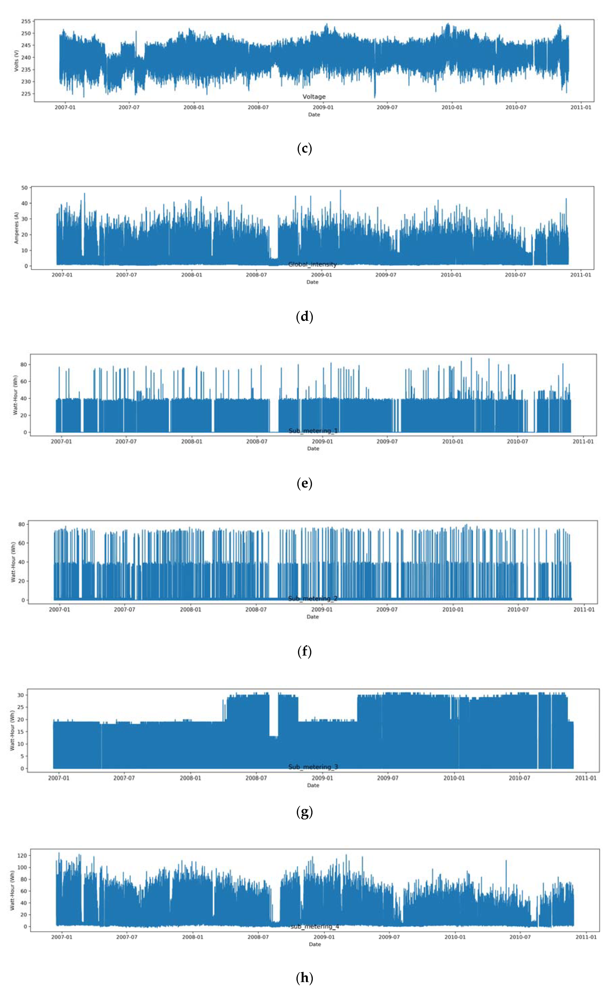
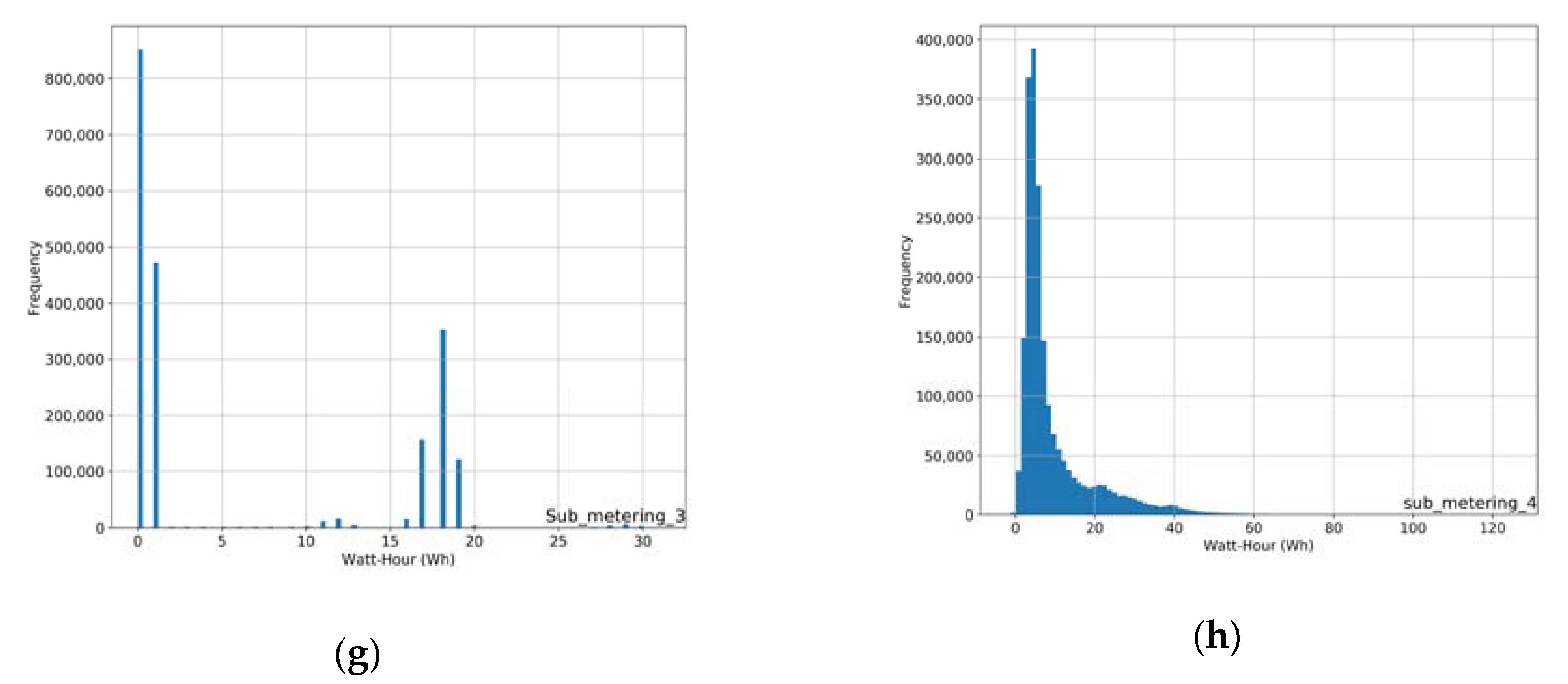
2.4. Data Exploration

In order to understand the data better, we used line plots for each feature (Figure 2) variable of the dataset and we consulted the augmented Dickey–Fuller test of [20] to deduce that the global active power is a stationary time series and therefore is not affected by seasonality. Afterwards, we examined the frequency distributions of the feature variables (Figure 3) by plotting histograms and concluded that global active power follows a bimodal distribution. It is interesting to note that the yearly distribution of global active power shows that active power is consistently bimodal (Figure 4) each year and as a result, a validation split based on that information would yield a test set that adequately represents the entirety of the data. Finally, we used the Pearson correlation metric (Figure 5) in order to check for the property of synchrony between the time series and we observed that global active power is synchronous with global intensity. As a result, we were able to test the impact of global intensity as an extra input variable in our neural networks.

2.5. Problem Formulation and Preprocessing

The first step in this comparative study was to define our research problem and make some initial hypotheses in order to frame the problem space properly. We selected to predict the next minute in the future from the minutely sampled data of the residential UCI dataset. We decided to frame this problem as a supervised learning task by implementing the sliding window method, as proposed by [33], so that our neural networks would be trained to learn a function that maps the input data points to an output. As an initial hypothesis, we considered this formulation in a real world setting where our trained models would be able to benefit an application which could take advantage of minutely predictions. In this scenario, we needed to select a window of lagged observations small enough so as not be affected by cold-start discrepancies. Moreover, the selection of a small window would also cover the main issue of high frequency predictions, which is the interpretation of relationships between data during the training phase of a neural network model. Since data points were sampled at a high rate, we needed to choose critical subsets of data points that clearly depict an upcoming peak, a valley or a more stable active power behavior on the next time step. A big set of data points at the input could lead to a wrong interpretation, since some of them could be interdependent or irrelevant to the predicted output.

Intuitively, we needed to select the smallest window of meaningful data points that would maximize temporal relevance. Since the selection of a single data point in the input may not provide valuable information about the behavior of the time series in the future, a set of two data points could help the neural networks identify patterns from the slope of the line that connects the data or from the level of fluctuations that occur between individual values. Therefore, we decided to set a window of two data points prior to the one that was about to be predicted as our input, on the assumption that these should be the most relevant data points giving us a clear connection to the output. It is certainly possible to conduct the same experiments with a larger input window. Consequently, the input of our neural network models consisted of two columns, the global active power at time $t-1$ and $t-2$. Since the global current intensity had high Pearson correlation with global active power, we added the global intensity at time $t-1$ and $t-2$ as input features on the base LSTM model in order to test the impact of synchrony as an additional experiment. The predicted output was the global active power at time $t$.

Before configuring the neural networks and building our models, we applied the following preprocessing transformations to the data:

• Values of input features were scaled between [0,1]. Min-max normalization was used in that interval through the MinMaxScaler class of SkLearn since neural networks handle input features well when they are on the same scale and the interval remains small;
• Two input columns were created based on the sliding window method.
• The dataset was split by allocating the first three years of observations to the training set and the last year to the test set. Since the distribution of global active power remains consistently bimodal, we believe that this is a proper holdout validation split;
• The training and test sets were split in input and output columns reshaped as the 3D format (samples, timesteps, features) for CNN and LSTM and (samples, features) for MLP, since it expects a 2D format.

2.6. Neural Network Configurations

In this study we configured the most prominent neural networks in time series forecasting and kept the activation and loss functions the same, as well as the compilation and training parameters, in order to derive a baseline performance. Therefore, we examined the behavior of the base LSTM network as well as the stacked and bidirectional variants. Furthermore, we compiled models for a 1D CNN and an MLP in order to compare more neural network architectures. As proposed in [20], neurons on the input layer of every model followed the dimensions of the feature columns and were equal to the window size we selected above. Every model had one hidden layer of 100 neurons and 1 neuron on the output layer. We selected 100 neurons as the hidden layer size because we wanted every network to have sufficient processing capacity. The size of the output layer was determined by the expected result. Therefore, one neuron in the output layer would predict the global active power at time $t$. Since the stacked LSTM architecture should contain more hidden layers, we decided to use one extra hidden layer with 100 neurons for our stacked LSTM model. Additional experiments were conducted on the stacked LSTM architectures where neurons would be dropped-out randomly with a probability of 0.2 in order to test the impact of regularization on more complex neural network structures.

The 1D convolutional network model contained a convolutional layer with 64 filters, a kernel size of 2, and the input was padded accordingly in order to obtain an output of the same length. Additionally, in our CNN architecture we added a pooling layer with a pool size of two in order to downsample the detected features. The pooling layer shared the same padding configuration as the convolutional layer. We proceeded to flatten the output of the pooling layer and use it as the input to a fully connected layer of 100 neurons. The predictions derived from the CNN model were obtained in the output layer. Last but not least, the MLP model had a simple structure of one input layer, one hidden layer, and one output layer, following the general configuration mentioned above.

The activation function used between the layers of every model was the rectified linear unit (ReLU). Moreover, we used the Mean Absolute Error (MAE) function to measure the loss, since this is a simple metric which denotes the absolute difference between the data and the model predictions. In addition, the Adam optimizer was used for adaptive learning rate optimization [34]. The training parameters for every model were considered with regard to optimal MAE values on the test set. Hence, we used holdout validation in order to use the first three years of data as the training set and the last year of data as the test set. This split was selected because we did not intend to tune the parameters of each model after training. In addition, more sophisticated validation techniques applicable to time series, such as nested cross-validation, would add unnecessary complexity to the comparison we attempted to examine. We acknowledge that the increased processing capacity of the hidden layers could cause increased total training times and a possible risk of overfitting. Therefore, in order to avoid overfitting, we stopped the training process and saved the models when the validation loss scores could not improve further, while their metrics were observed simultaneously in the notion of logical conjunction on the same epoch interval. After the eighth epoch the validation loss of any individual model was at least slightly worse than the best loss observed in that eight-epoch interval for that same model. As a result, the neural network models were trained after eight epochs with a batch size of 72 training samples.

3. Results

As a result of the above configurations we evaluated the performance of our models from the values of the loss function on the training and test set. In Figure 6, we present the graphs containing a sample of 150 global active power data points from the test set and 150 predicted data points generated by each neural network model, in order to visualize the robustness of our predictions on each time step. Moreover, in Figure 7, we present the graph panel containing the loss function values throughout the training process of each neural network model. The examined models performed well when trying to predict the global active power from the unknown data in the test set since the data points at the same time step neither diverged drastically nor did they follow an unusual pattern. However, we can observe that when a peak or a valley occurred in the test data, the models made a less accurate prediction, resulting in greater deviation from the actual active power data points in the same time interval. A distinct example of this phenomenon can be detected in the region between the 45th and 55th data points, where the predicted value for the power peak was lower than the actual test value. Through this example, we are also able to notice the difference in the quality of predictions among our neural network models. The stacked LSTM model made the least accurate peak prediction in that region, while other models, such as the 1D CNN and MLP, were able to achieve approximations closer to the actual peak value. These observations can be generalized to the entirety of the dataset, since it is indeed difficult to anticipate peaks and valleys in such a short prediction horizon when only the most recent and most relevant data points of the same feature are considered.

Furthermore, the graphs of the training and test loss show that we avoided overfitting and underfitting with that configuration, since the curve of validation loss was always below the curve of training loss. The curves of the training loss function in each graph show that there was a steady improvement of the prediction quality throughout the training process, whereas the validation loss curves show that after a small number of epochs no further improvement could be achieved when testing the models on unknown data, given those configuration parameters. It is interesting to note that models with inferior training loss results, such as the 1D CNN, had a decent performance on unknown data and were able to fit the data reasonably well in regions where peaks and valleys occurred.

Table 1. Neural networks’ training and testing scores.

Scores	MLP	1D CNN	Baseline LSTM	Baseline LSTM (Synchrony)	Stacked LSTM (No Dropout)	Stacked LSTM (Dropout 0.2)	Bidirectional LSTM
Train Score (Loss)	0.00797	0.00846	0.00798	0.00826	0.00824	0.00839	0.00808
Test Score (Loss)	0.00670	0.00716	0.00672	0.00701	0.00689	0.00711	0.00677

presents the evaluation metrics for every neural network type on the training and test sets. After examining the overall error loss function scores of each model, we deduced that the top performing ones were the MLP and the Baseline LSTM. Since the LSTM network is more suitable for handling temporal relationships, we re-ran the experiment by adding the extra feature of global current intensity in order to test the impact of synchrony and we observed a decrease in training time. Furthermore, we ran tests by adding dropout to the stacked LSTM variant, since its initial performance on unknown data was the worst when compared to other LSTM models, but that change did not yield better results. Finally,

Table 2. Average training time per epoch for each neural network configuration.

Neural Network Type	Average Training Time per Epoch (Seconds)
MLP	20
1D CNN	42
Baseline LSTM (Synchrony)	98
Baseline LSTM	120.25
Stacked LSTM	165.25
Bidirectional LSTM	269.5

shows the average training time of each model and we observed that MLP was able to converge to an acceptable mapping of the input to the output faster than the other network models. It is, therefore, interesting to note that some of the more complex LSTM variants went through a distinctly slower training process.

4. Discussion

This work presented the baseline performance comparison of neural network models for minutely active power forecasts derived from residential data. In our supervised learning formulation of this high frequency forecasting problem we observed that the multi-layer perceptron performed best in terms of loss and average training time. Since MLP follows a simpler structure and recognizes a 2D data format we can deduce that due to the selection of a small and relevant set of input data points, the network was able to converge fast, producing fairly accurate predictions in the output. The long short-term memory network and its variants converged slower, possibly due to their computational complexity, since the data relationships that we wanted to identify did not refer to data points far into the past. We expect changes to the training and test scores when the window size and the number of input variables increase and anticipate that LSTMs will be able to produce accurate predictions at a higher complexity.

Our study could be useful in approaching high granularity forecasts with machine learning methods. Since the baseline performance of neural networks was evaluated and minutely sampled energy data was explored, we now have a starting point for further parameter tuning and experimentation. Future work could apply grid search techniques [35] for hyperparameter optimization in order to improve our baseline models. It would also be useful to explore the potential of modular solutions combining the neural networks we studied here in a pipeline-like structure, in order to investigate whether other important aspects of the highly granular time series forecasting in the energy sector emerge. For example, more complex neural network architectures could utilize these models in order to enrich a dataset at the input module or in order to derive partial predictions based on different criteria in parallelly working modules.

References

1. Magoutas, B.; Apostolou, D.; Mentzas, G. Situation-aware Demand Response in the smart grid. In Proceedings of the 2011 16th International Conference on Intelligent System Applications to Power Systems, Hersonissos, Greece, 25–28 September 2011; pp. 1–6. [Google Scholar] [CrossRef]
2. Rantou, K. Missing Data in Time Series and Imputation Methods. Master’s Thesis, University of the Aegean, Lesbos, Greece, 2017. [Google Scholar]
3. Waser, M. Nonliniear Dependencies in and between Time Serie. Master’s Thesis, Vienna University of Technology, Vienna, Austria, 2010. [Google Scholar]
4. Verleysen, M.; Francois, D. The Curse of Dimensionality in Data Mining and Time Series Prediction. Comput. Vis. 2005, 3512, 758–770. [Google Scholar] [CrossRef]
5. Deep Learning for Time Series and Why DEEP LEARNING? Medium. 2020. Available online: https://towardsdatascience.com/deep-learning-for-time-series-and-why-deep-learning-a6120b147d60 (accessed on 26 March 2020).
6. Hua, Y.; Zhao, Z.; Li, R.; Chen, X.; Liu, Z.; Zhang, H. Deep Learning with Long Short-Term Memory for Time Series Prediction. IEEE Commun. Mag. 2019, 57, 114–119. [Google Scholar] [CrossRef] [Green Version]
7. Koprinska, I.; Wu, D.; Wang, Z. Convolutional Neural Networks for Energy Time Series Forecasting. In Proceedings of the 2018 International Joint Conference on Neural Networks (IJCNN), Rio de Janeiro, Brazil, 8–13 July 2018; pp. 1–8. [Google Scholar]
8. Shiblee, M.; Kalra, P.K.; Chandra, B. Time Series Prediction with Multilayer Perceptron (MLP): A New Generalized Error Based Approach. In Computer Vision; Springer: Berlin/Heidelberg, Germany, 2009; Volume 5507, pp. 37–44. [Google Scholar]
9. Alamaniotis, M.; Tsoukalas, L.H. Anticipation of minutes-ahead household active power consumption using Gaussian processes. In Proceedings of the 2015 6th International Conference on Information, Intelligence, Systems and Applications (IISA), Corfu, Greece, 6–8 July 2015; pp. 1–6. [Google Scholar]
10. Singh, S.; Hussain, S.; Bazaz, M.A. Short term load forecasting using artificial neural network. In Proceedings of the 2017 Fourth International Conference on Image Information Processing (ICIIP), Waknaghat, India, 21–23 December2017; pp. 1–5. [Google Scholar]
11. Kuo, P.-H.; Huang, C.-J. A High Precision Artificial Neural Networks Model for Short-Term Energy Load Forecasting. Energies 2018, 11, 213. [Google Scholar] [CrossRef] [Green Version]
12. Hossen, T.; Nair, A.S.; Chinnathambi, R.A.; Ranganathan, P. Residential Load Forecasting Using Deep Neural Networks (DNN). In Proceedings of the 2018 North American Power Symposium (NAPS), Fargo, ND, USA, 9–11 September 2018; pp. 1–5. [Google Scholar] [CrossRef]
13. Zhang, D.; Han, X.; Deng, C.; Taiyuan University of Technology; China Electric Power Research Institute. Review on the research and practice of deep learning and reinforcement learning in smart grids. CSEE J. Power Energy Syst. 2018, 4, 362–370. [Google Scholar] [CrossRef]
14. Kampelis, N.; Tsekeri, E.; Kolokotsa, D.; Kalaitzakis, K.; Isidori, D.; Cristalli, C. Development of Demand Response Energy Management Optimization at Building and District Levels Using Genetic Algorithm and Artificial Neural Network Modelling Power Predictions. Energies 2018, 11, 3012. [Google Scholar] [CrossRef] [Green Version]
15. Koponen, P.; Hänninen, S.; Mutanen, A.; Koskela, J.; Rautiainen, A.; Järventausta, P.; Niska, H.; Kolehmainen, M.; Koivisto, H. Improved modelling of electric loads for enabling demand response by applying physical and data-driven models: Project Response. In Proceedings of the 2018 IEEE International Energy Conference (ENERGYCON), Limassol, Cyprus, 3–7 June 2018; pp. 1–6. [Google Scholar]
16. Ahmad, A.; Javaid, N.; Mateen, A.; Awais, M.; Khan, Z.A. Short-Term Load Forecasting in Smart Grids: An Intelligent Modular Approach. Energies 2019, 12, 164. [Google Scholar] [CrossRef] [Green Version]
17. Walther, J.; Spanier, D.; Panten, N.; Abele, E. Very short-term load forecasting on factory level–A machine learning approach. Procedia CIRP 2019, 80, 705–710. [Google Scholar] [CrossRef]
18. Zhu, J.; Yang, Z.; Mourshed, M.; Li, K.; Zhou, Y.; Chang, Y.; Wei, Y.; Feng, S. Electric Vehicle Charging Load Forecasting: A Comparative Study of Deep Learning Approaches. Energies 2019, 12, 2692. [Google Scholar] [CrossRef] [Green Version]
19. Deep Learning for Time Series Forecasting: The Electric Load Case, GroundAI. 2020. Available online: https://www.groundai.com/project/deep-learning-for-time-series-forecasting-the-electric-load-case/1 (accessed on 26 March 2020).
20. Time Series Analysis, Visualization & Forecasting with LSTM, Medium. 2020. Available online: https://towardsdatascience.com/time-series-analysis-visualization-forecasting-with-lstm-77a905180eba (accessed on 14 February 2020).
21. Neural Networks Over Classical Models in Time Series, Medium. 2020. Available online: https://towardsdatascience.com/neural-networks-over-classical-models-in-time-series-5110a714e535 (accessed on 14 February 2020).
22. LSTM for Time Series Prediction, Medium. 2020. Available online: https://towardsdatascience.com/lstm-for-time-series-prediction-de8aeb26f2ca (accessed on 14 February 2020).
23. UCI Machine Learning Repository: Individual Household Electric Power Consumption Data Set, Archive.ics.uci.edu. 2020. Available online: https://archive.ics.uci.edu/ml/datasets/individual+household+electric+power+consumption (accessed on 14 February 2020).
24. Perceptron Learning Algorithm: A Graphical Explanation of Why It Works, Medium. 2020. Available online: https://towardsdatascience.com/perceptron-learning-algorithm-d5db0deab975 (accessed on 26 March 2020).
25. Multilayer Perceptron—DeepLearning 0.1 Documentation, Deeplearning.net. 2020. Available online: http://deeplearning.net/tutorial/mlp.html (accessed on 26 March 2020).
26. CS231n Convolutional Neural Networks for Visual Recognition, Cs231n.github.io. 2020. Available online: http://cs231n.github.io/convolutional-networks/ (accessed on 26 March 2020).
27. LeNail, A. NN-SVG: Publication-Ready Neural Network Architecture Schematics. J. Open Source Softw. 2019, 4, 747. [Google Scholar] [CrossRef]
28. Recurrent Neural Network—An Overview|ScienceDirect Topics, Sciencedirect.com. 2020. Available online: https://www.sciencedirect.com/topics/engineering/recurrent-neural-network (accessed on 26 March 2020).
29. Understanding LSTM Networks—Colah’s Blog, Colah.github.io. 2020. Available online: https://colah.github.io/posts/2015-08-Understanding-LSTMs/ (accessed on 26 March 2020).
30. How to Select the Right Evaluation Metric for Machine Learning Models: Part 1 Regression Metrics, Medium. 2020. Available online: https://medium.com/@george.drakos62/how-to-select-the-right-evaluation-metric-for-machine-learning-models-part-1-regrression-metrics-3606e25beae0 (accessed on 26 March 2020).
31. Dimkonto/Minutely-Power-Forecasting, GitHub. 2020. Available online: https://github.com/dimkonto/Minutely-Power-Forecasting (accessed on 15 February 2020).
32. Ebeid, E.; Heick, R.; Jacobsen, R. Deducing Energy Consumer Behavior from Smart Meter Data. Futur. Internet 2017, 9, 29. [Google Scholar] [CrossRef] [Green Version]
33. Brownlee, J. How to Develop Multi-Step LSTM Time Series Forecasting Models for Power Usage, Machine Learning Mastery. 2020. Available online: https://machinelearningmastery.com/how-to-develop-lstm-models-for-multi-step-time-series-forecasting-of-household-power-consumption/ (accessed on 16 February 2020).
34. Kingma, D.; Ba, J. Adam: A Method for Stochastic Optimization. In Proceedings of the 3rd International Conference for Learning Representations, San Diego, CA, USA, 7–9 May 2015; Available online: https://arxiv.org/abs/1412.6980v8 (accessed on 9 April 2020).
35. An Intro to Hyper-Parameter Optimization Using Grid Search and Random Search, Medium. 2020. Available online: https://medium.com/@cjl2fv/an-intro-to-hyper-parameter-optimization-using-grid-search-and-random-search-d73b9834ca0a (accessed on 24 February 2020).
Figure 1. Convolutional neural network architecture illustration created using the NN-SVG online schematics tool found in [27].
Sustainability 12 03177 g001
Figure 2. Line plots of dataset features. Since each feature is a time series, the y-axis represents the unit of each feature, and x-axis represents the date. (a) Global household active power. (b) Global household reactive power. (c) Household voltage. (d) Global household current intensity. (e) Kitchen energy consumption. (f) Laundry room energy consumption. (g) Consumption of electric water-heater and air-conditioner. (h) Remaining energy consumption measurements not covered by the sub-metering information.
Sustainability 12 03177 g002aSustainability 12 03177 g002b
Figure 3. Histogram of feature distributions (100 bins). The y-axis represents the number of occurrences and the x-axis represents the unit of each feature. (a) Global household active power. (b) Global household reactive power. (c) Household voltage. (d) Global household current intensity. (e) Kitchen energy consumption. (f) Laundry room energy consumption. (g) Consumption of electric water-heater and air-conditioner. (h) XXXRemaining energy consumption measurements not covered by the sub-metering information.
Sustainability 12 03177 g003aSustainability 12 03177 g003b
Figure 4. Yearly distribution of global active power. The y-axis represents the number of occurrences and the x-axis represents the unit of global active power (kW). (a) Global active power distribution in 2007 (b) Global active power distribution in 2008 (c) Global active power distribution in 2009 (d) Global active power distribution in 2010.
Sustainability 12 03177 g004
Figure 5. Pearson correlation between dataset features. The labels of this 2D array are the names of the dataset features. A positive correlation of 1 is represented by yellow and a negative correlation of −1 is represented by blue.
Sustainability 12 03177 g005
Figure 6. Prediction evaluation on 150 data points for (a) Long Short-Term Memory (LSTM) network, (b) Stacked LSTM, (c) Bidirectional LSTM, (d) 1-Dimensional Convolutional Neural Network (1D CNN), (e) Multilayer Perceptron (MLP). The red line represents the data points of the test set and the blue line represents the data points predicted by each model on the same time step. On the y-axis we set the unit of global active power (kW) and on the x-axis we enumerated the data points.
Sustainability 12 03177 g006
Figure 7. Loss function on train and test set for eight epochs of training on (a) LSTM, (b) Stacked LSTM, (c) Bidirectional LSTM, (d) 1D CNN, (e) MLP. The blue line represents the loss function during training and the orange line represents the loss function during validation. On the y-axis we set the values of the loss function and on the x-axis, we enumerated the epochs.
Sustainability 12 03177 g007