With about 1.21 billion in population in 2011, India was one of the second largest countries after China in terms of size of population [
21]. Although the present share of the urban population in India is relatively small, namely about 31.2%, but it is quite large in absolute number, namely, about 377 million [
22]. Furthermore, the decadal growth of urban population in India, though with a lower base, has been higher than the growth rate of the rural population from 1931 onwards (
Table 1). The differences in the growth rates of the urban and rural population have been quite significant in some of the past decades. For instance, in 1951, mainly due to immigration of population from Pakistan (also due to religious riots), many people moved to urban areas where safety was higher; and in later years, the urbanization has reached its own momentum of growth due to (i) migration from rural to urban areas, (ii) the identification of new settlements as urban (There have been some changes in the definition of ‘urban’ over the years, and these changes have impacted the number of settlements declared as urban. However, it is not possible to reconstruct the past data with the revised definitions, therefore, the number of towns and urban population as published by Census of Indian 2011 for the years 1901 to 2011 have been used in this study. In India, prior to 1951, the definition of urban was arbitrary. An urban center was identified on the bases of (i) urban local body or municipality, (ii) civil lines, which were outside the boundary of municipality/local body, and (iii) all the cantonments and all other contiguous clusters of houses inhabited by 5000 or more number of persons. In this identification, the Census superintendent was empowered to take a decision to declare a settlement as urban, keeping in mind the density of dwellings, historic nature of the settlement, importance of the settlement in trade, and to avoid declaring an overgrown village (without urban characteristic) as a town [
23]. The Census of 1951 used the following criteria to define a settlement as urban: (i) Population not less than 5000, and (ii) settlements with less than 5000 population, but having urban characteristics like supply of drinking water, electricity, schools, post offices, hospitals, etc. Census superintendents were empowered to take decisions for declaring and identifying settlements as urban based on these characteristics. In 1961, more strict criteria to identify ‘urban’ was adopted, and these were: (a) Statutory towns—all places with statutory bodies like city corporation, municipality, cantonment boards, or a notified town area committee, (b) census towns—all the places which satisfied the following criteria: (i) Population of 5000 and above; (ii) density of population not less than 400 persons per square kilometer; and (iii) at least 75% of male population engaged in non-agricultural work [
24]. A small change in this definition of census towns was brought in 1971, in which the b(iii) criterion was changed to ‘at least 75% of the male main working (a worker is main worker if he/she has worked for not less than 183 days in the year preceding the census) population engaged in a non-agricultural sector. Since 1971, there has not been any change in the definition and criteria of identification of ‘urban’ by the Census of India [
22]. The changes of definition in 1951 and 1961 led to a decline in the number of towns from 3060 in 1951 to 2700 in 1961 (see [
25] for details). India added 2774 new Census Towns in 2011, more than in any previous censuses without any revision in definition adopted in 1971. Some researchers have called this ‘Census activism’ [
26].), and (iii) the natural increase in urban population.
3.1. Size-Class Distribution
India’s urban system is top-heavy. That is, a few mega-urban centers accommodate a significantly higher proportion of the total urban population than those by medium and small cities. This top-heavy system has emerged because of the nature of historical experience the Indian economy went through. In the colonial period (roughly mid-19th century to mid-20th century), the port and capital cities acquired major importance. The port cities became major conduit of exports and imports, and in this way Kolkata, Mumbai, and Chennai emerged. Later on, industries—particularly, textile and, after independence, petrochemical industries—also started locating themselves in these urban centers, attracting workers from neighboring regions. Till today, these cities remain major urban centers in their respective regions and also centers of economic opportunities. Delhi—due to political factors, as capital city—started growing, while later educational institutions and industries started locating in and around Delhi. Today, Delhi has emerged as one of the biggest conurbation regions of India, including many negative externalities.
With the economic opportunities diffusing and given the large geographical surface of the country, other secondary urban centers in India also started emerging, giving rise to a second layer: Bangalore, Pune, Nashik, Hyderabad, Mangalore, etc. The top-heaviness of the urban system has not only persisted over the years, but it has also sharpened. This can well be seen from the fact that, though there are a large number of towns in India (see
Table 2), the major share of the urban population has been in Class I cities (population of 100,000 and above), whose total share in the total number of towns is significantly small; for instance, it was only 7.6% in 2011, but these towns had 70.2% of the total urban population (
Table 3). The share of other classes of the towns in the total urban population has over the years declined, but their share in the total number of towns, except class VI, has increased. In fact, as we shall see in the following sections, the economic importance of large cities (million plus cities) have consistently increased. The number of million plus cities in India rose from 5 (with a share of the total urban population of 18.81%) in 1951 to 23 (32.54% of the urban population) in 1991, and to 53 (42.62% of the urban population) in 2011 (see
Table 4).
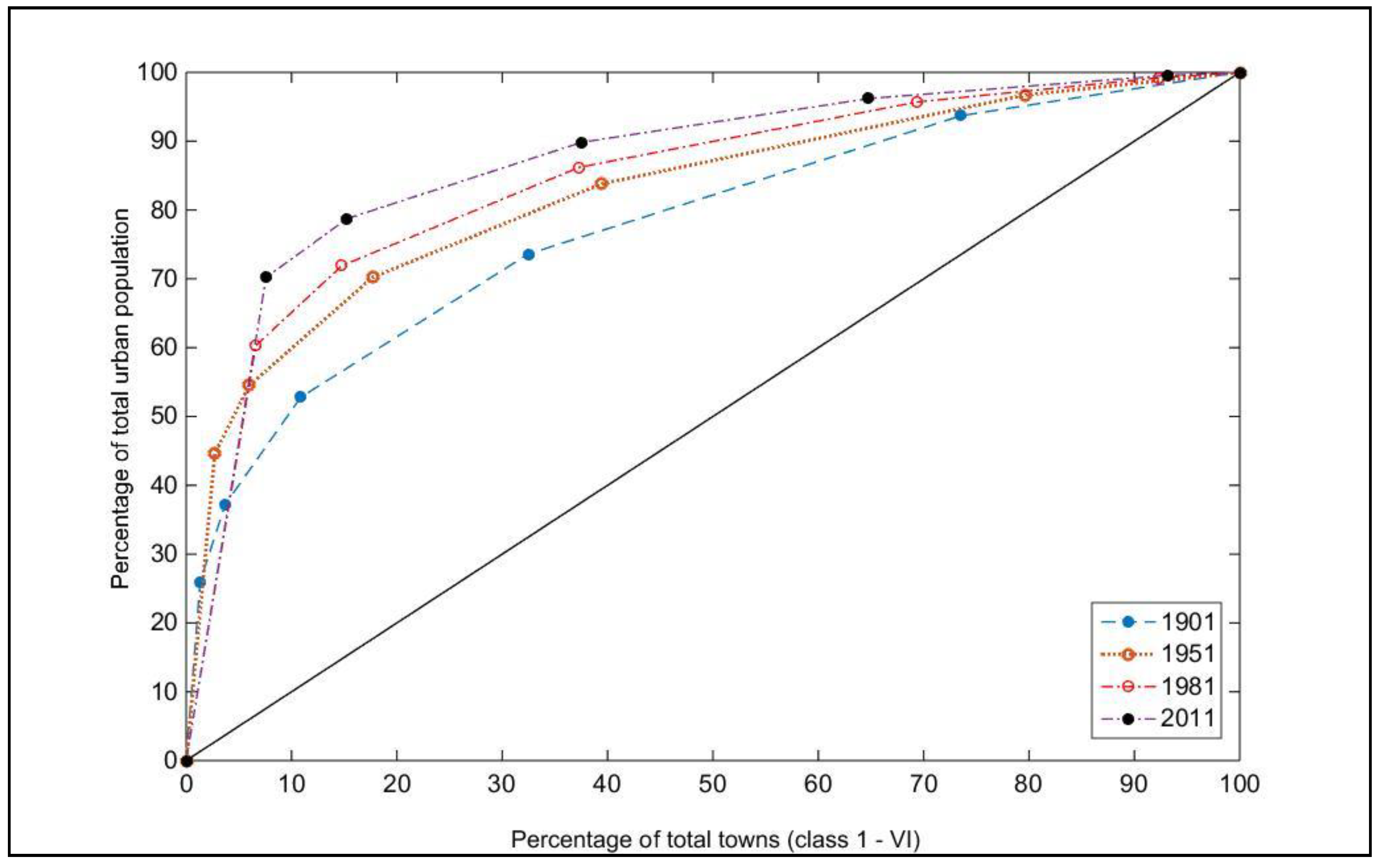
This consistent strengthening of ever-increasing large cities in the urban system in India is well illustrated by the Lorenz curve in
Figure 1. The Indian urban system—in terms of distribution of population in different size-class of cities—has clearly become more unequal. The small and medium cities’ share in total urban population has consistently declined over the years, and that is why the Lorenz curves for the selected years plotted in
Figure 1, have progressively shifted away from the diagonal (or the line of equality). As a consequence, and parallel to his observation, the Gini coefficient has increased consistently (
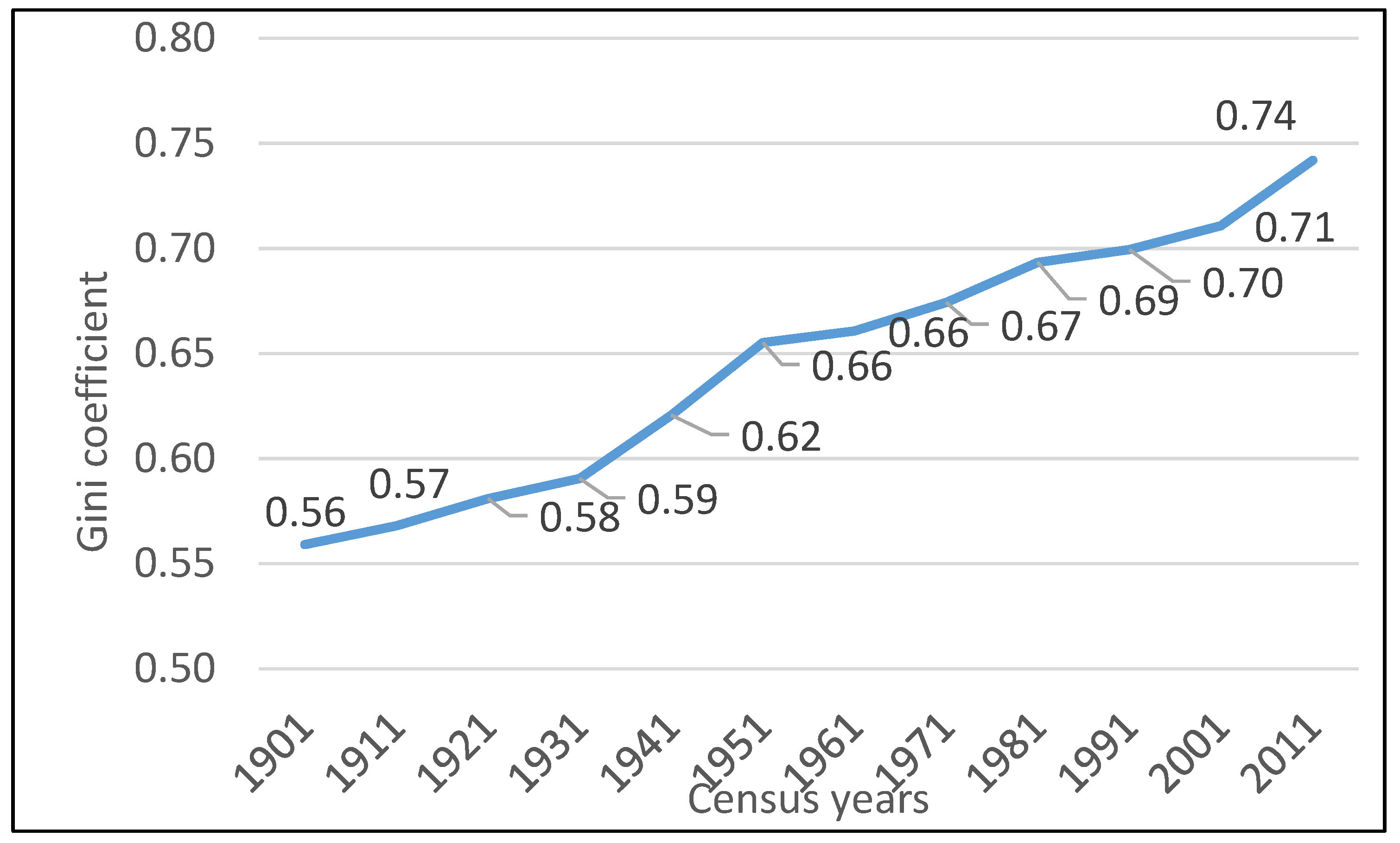
Figure 2). The higher increases in the coefficient occurred in 1941, 1951, 1961, and 2011, when the share of population of Class I cities increased substantially. The share of Class I cities in the total urban population was 31.2% in 1931, it increased to 38.2% in 1941, 51.4% in 1961, and 57.2% in 1971. As mentioned above, the share of Class I cities further consolidated between 2001–2011. It has increased to 70.2%, in 2011, of the total urban population in the country from 68.6% in 2001.
3.2. Rank-Size Rule
The hierarchical distribution of cities and their rank orders within a country have been one of the important areas of research in urban systems studies. Empirical analyses have supported this idea that generally the hierarchy of cities in a country conforms to what [
27] is called the rank-size rule distribution of cities. In an urban system conforming to a rank-size rule distribution, the population of
nth order city (
Pn), in descending order of population, is:
or
where
P1 is the population of the highest-order city, that is, the rank 1 city with the highest volume of population;
is ordinal rank number of the observed city. If we take the log of the rank and the population of the towns and plot the results on an x-y axis, we observe a straight-line distribution. When we take the log of both sides of Equation (1), we can write Equation (1) as:
This, as mentioned above, gives rise to a linear functional correlation between the population of the cities and the rank of these cities. This functional relationship can also be presented in a regression equation with
Y as a rank of the towns, constant (
α), and population as
X,
This implies that if the urban system of a country follows a rank-size rule distribution, the estimated coefficient of the downward sloping line will be −1; higher values (−1 to 0) will indicate that bigger cities are disproportionately larger and have a large share of the total urban population, while values less than −1 indicate that the population is dispersed in a large number of cities [
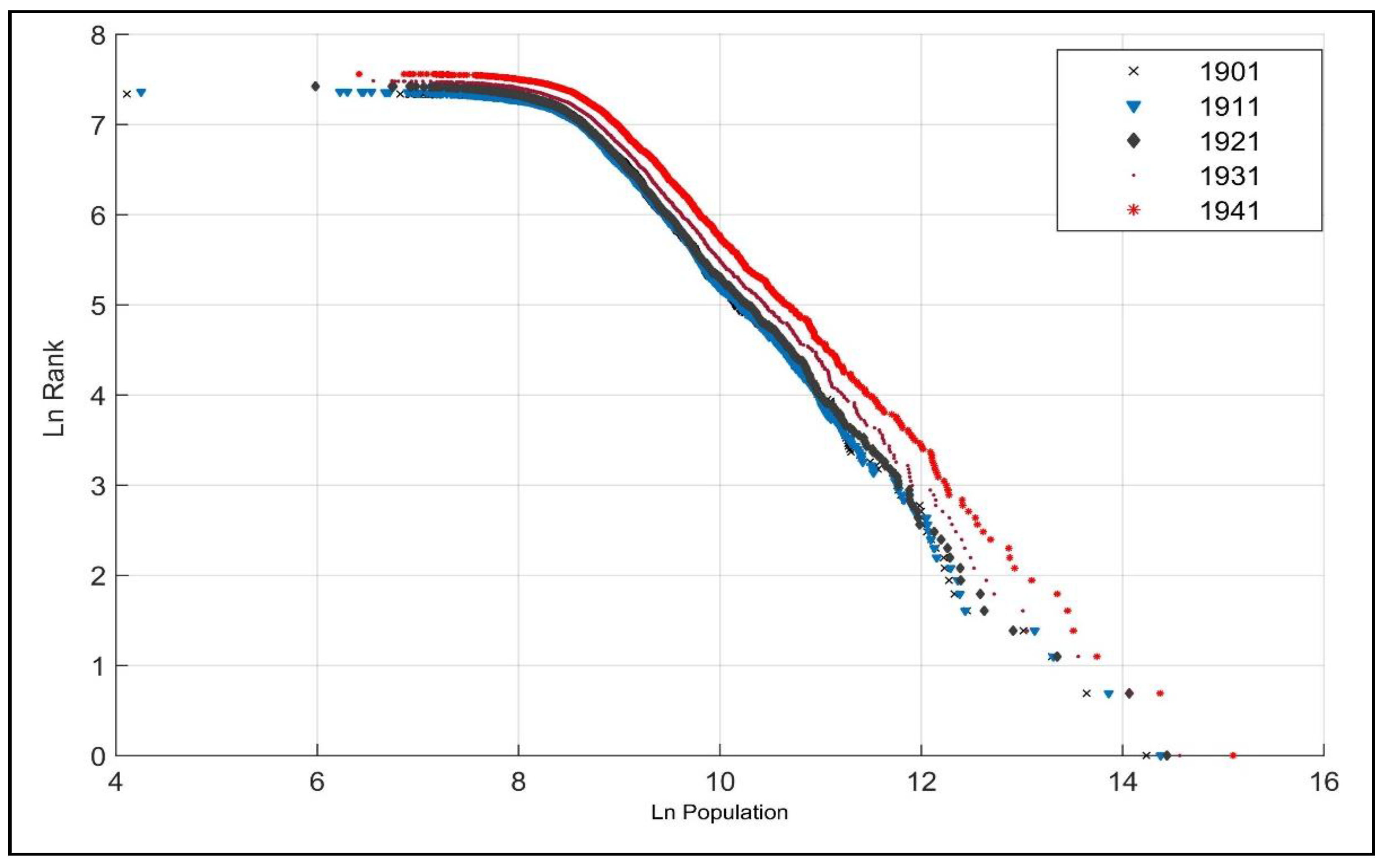
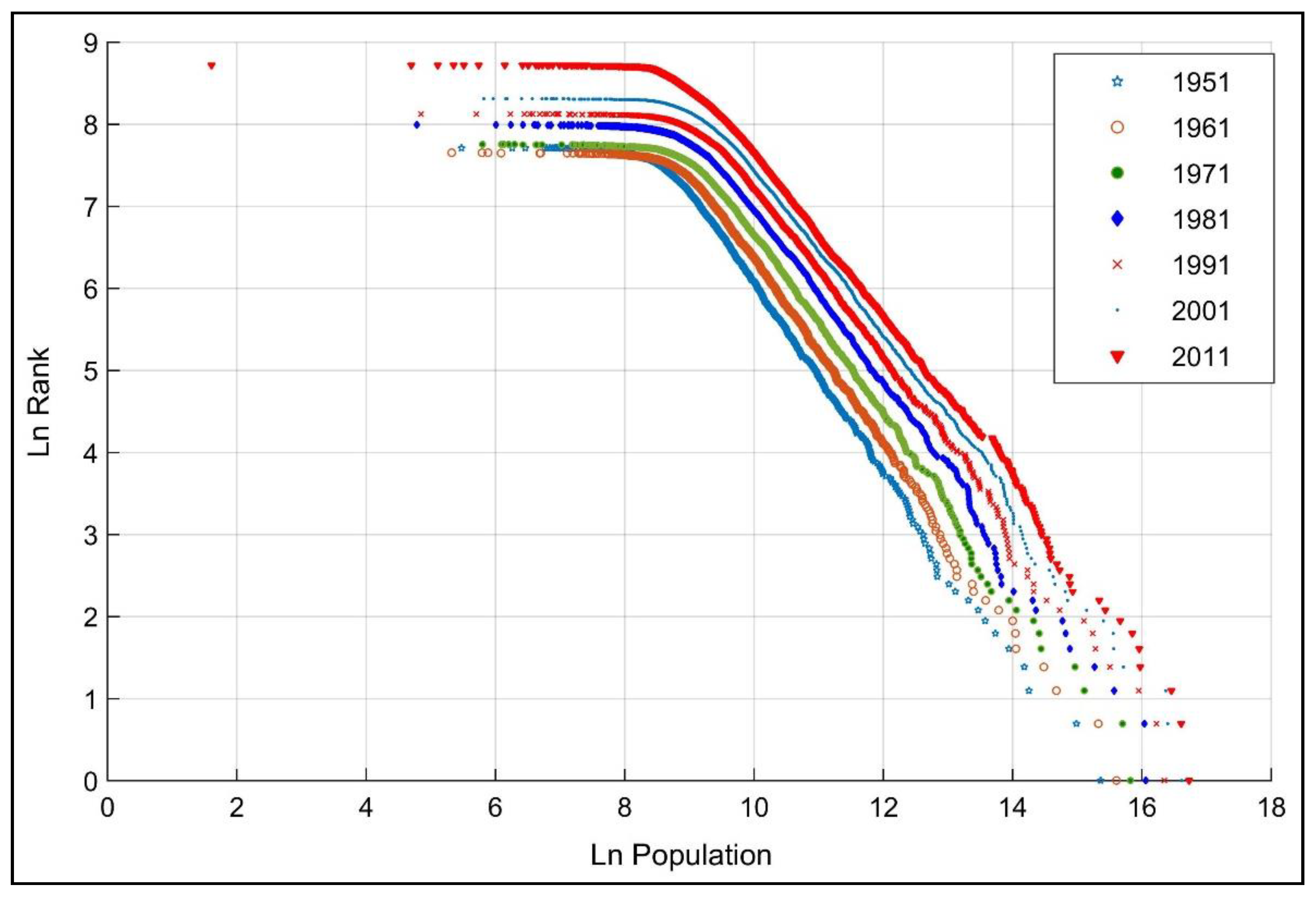
28]. The empirical results of the rank-size distribution of Indian cities over the period 1901–2011 can be found in
Figure 3 and
Figure 4.
In general, the rank-size rule distribution of cities is mostly found in developed countries where there is a relatively balanced regional development. It is plausible to expect that spatially unbalanced developed economies will lead to a migration of population to bigger cities, giving rise to a lower share of the population in lower-order cities in comparison to what is generally expected from the rank-size rule distribution. The concentration of a larger share of the population in top rank cities is also called primacy of these cities. If the rank 1 city has more than double of the population of the 2nd order city (as expected under a rank-size rule distribution), it is called the primate city. Commonly, the primacy of the city of rank 1—denoted as
C1—is measured as the ratio between
P1 and
P2, as presented below:
According to the rank-size rule:
Thus, the population of a rank 1 city is equal to the sum of the population of rank 2, rank 3, and rank 4 cities. Therefore, we can also use the ratio between population of rank 1 city and the sum of the population of ranks 2–4 to find out whether they are equal to 1 (no primacy) or have a primacy, denoted as C2, in relation to the 3 lower-order cities. This ratio also helps us to find out the distribution of the population in the 4 top cities and their imbalances, if any, within.
The rank-size rule distribution of the Indian cities from 1901 to 2011 are presented in
Figure 3 and
Figure 4. It is evident from these figures that over the years there have been definite orders of these cities close to the rank-size rule, but there is also a huge concentration of cities with a low population size at the lower end, with the log of ranks 7–9 having a log of the population of 4.0–8.5.
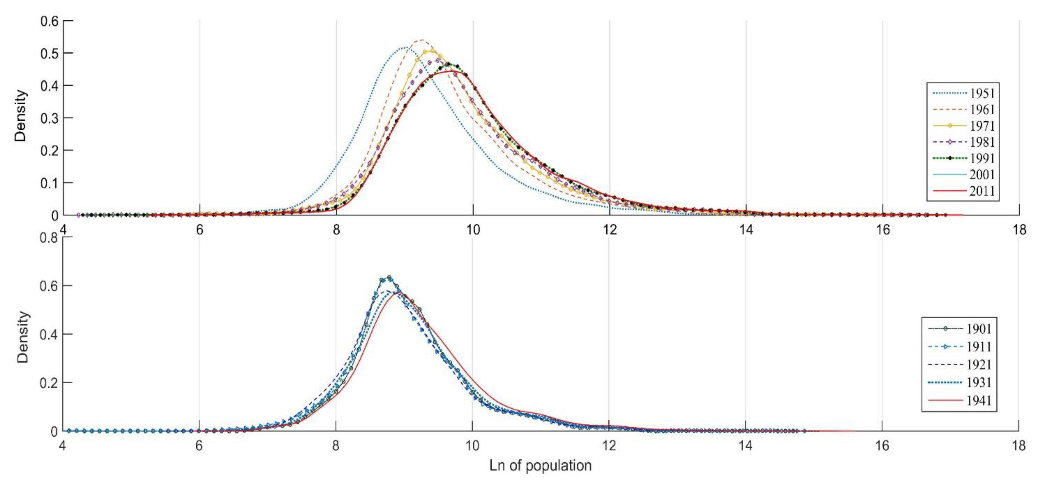
Figure 5—with the urban kernel density function—shows that the highest number of cities was located in the band of the log of population 8.0 to 10.0, although in later years, with an increase in the population of cities, it has shifted to the band of about log 8.0 to 12.0. Further, there seems to be largely a log-normal distribution of cities which is found in the rank-size rule conformity of the urban hierarchy.
The regression results produced in
Table 5 show that in India from 1901 till 2011, the urban system has followed the rank size rule, but the primacy has been strengthening (the regression coefficient has increased over the years). The Zipf coefficient or β values have increased from −1.099 (nearly in conformity with the rank-size rule) in 1901, to −0.959 in 1951 to −0.854 in 2011, showing that city size distribution in India has progressively and steadily moved away from a rank-size rule distribution towards a dominance of large cities. That means the slope of the lines have become flatter over the years. It is not, therefore, any surprise to see that the size of the largest city population has also risen over the years. In 1901, the size of the largest city (UA) in the total urban population was 1.52 million, which increased to 4.69 million in 1951, and further increased to 18.39 million in 2011. The share of the top five cities (UA) in the total urban population has also increased from 14.15% to 20.82% in 1971, and thereafter it has declined to reach 17.50% in 2011 (
Table 6). Further, there have not been many differences in the size of the top three cities in terms of population in 2001 and 2011, while during 1951–1991 the top three cities had a rather similar population size. This shows that there is not one city dominance in India, but a group of top cities. Given the large geographical size of India and the lop-sided regional economic development [
29], this is plausible. Linsky [
30] has pointed out that primacy will be more prominent in countries with small territorial extents, but it is noteworthy that India has a large territorial extent. However, the states in India are of the size of many European countries and, as such, the polarized development within the individual states has created a primacy within these states. In all major states of India, a few major cities have a disproportionally large population, for instance, Mumbai in Maharashtra, Kolkata in West Bengal, Chennai in Tamil Nadu, and Hyderabad in Telangana. Given the fact that in India, there is a group of large cities, the primacy indices, both
C1 and
C2, are, except in 1941, lower than expected as per the conventional rank-size rule (
Table 6).
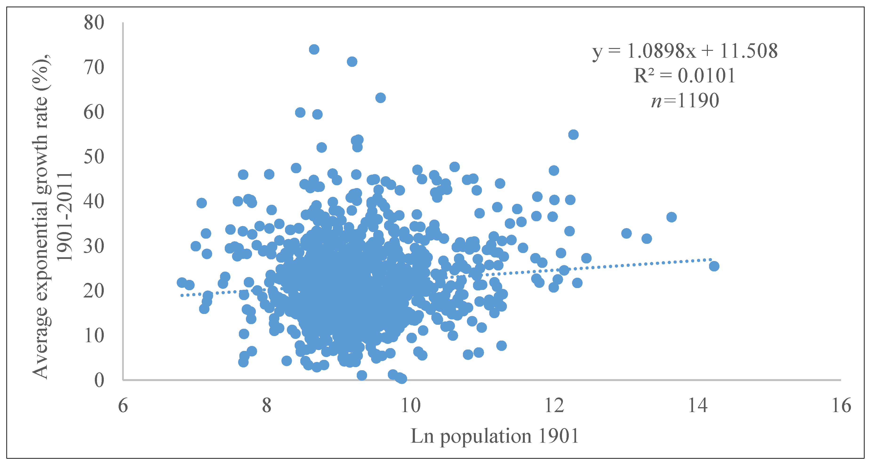
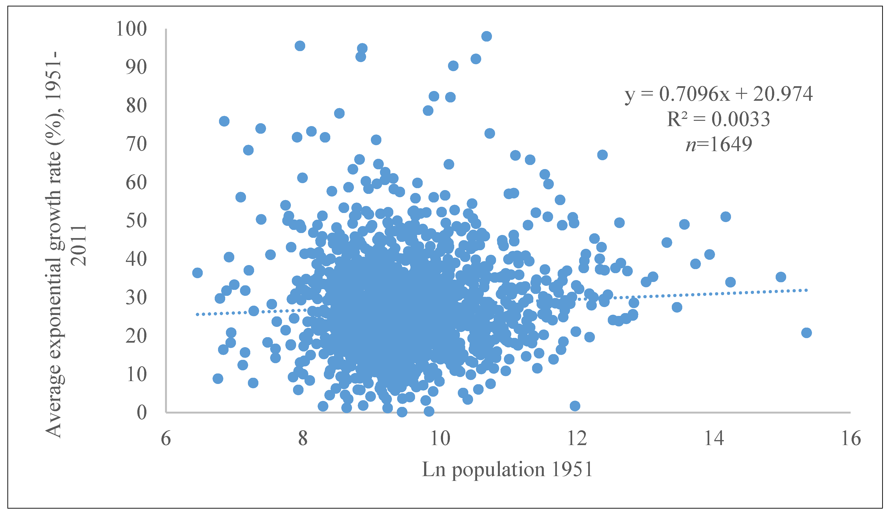
Another, often reported, empirical regularity about cities addresses the proportionate growth of cities. This regularity shows that there is generally no correlation between the size of cities and their population growth rates. The small and big cities grow largely at random rates. This means that the underlying stochastic process of growth is the same for all cities. This is a well-known proposition by Gibrat [
31], which was originally put forward by the astronomer Kapteyn [
32], who stated, “a stochastic growth process that is proportionate gives rise to an asymptotically lognormal distribution” [
33]. In India, the number of cities has risen over the years and therefore, the growth rates can be computed based on the regularities of the cities. We note that many cities have been de-classified or that their names are not matching over the years, and therefore, they have been dropped from the computation of growth rates. We computed the growth of 1190 cities for 1901–2011, and of 1649 cities for 1951–2011 based on the regularity of population data. The growth rates of population are plotted against the
log of population of these cities in
Figure 6 and
Figure 7. These results show that the Indian urban system follows the Gibrat’s proportionate growth thesis. This also means that cities will most likely not converge in terms of their population.


