Dynamic Input–Output Analysis of a Carbon Emission System at the Aggregated and Disaggregated Levels: A Case Study in the Northeast Industrial District

Abstract

Research on carbon emissions of complex interactive activities in urban agglomerations is one of the hotspots of global climate change research. A comprehensive analysis of the urban agglomeration system’s carbon emissions is essential to reveal strategies for reduction and support sustainable development. The objective of this research is to develop an integrated carbon emission network model to explore the impact of different energy types on the Northeast Industrial District (NID), China. Four representative energy groups are considered. Specifically, at the aggregated sector-level, this research quantified the relative contributions of socioeconomic factors to carbon emission changes using structural decomposition analysis and examined the system efficiency and redundancy through robustness analysis. At the disaggregated level, the research investigated carbon emissions of different sectors from production-based, consumption-based, and income-based viewpoints. Moreover, emissions from specific categories of final demand and primary input were quantified. It was found that the increase of final demand level will proceed to push up the carbon emissions of the NID. Changing the production structure contributes to reducing emissions. The carbon emissions system has a high redundancy and low efficiency, illustrating that there are many emission pathways within the system. In addition, the use of crude oil significantly increases system redundancy and inhibits system efficiency. However, the major limitation of the model is that the long-term changes of the system are not considered. Moreover, considering the actual policies, emission reduction simulations could be added in the future.

1. Introduction

Carbon dioxide (CO₂) emissions are mainly produced by socioeconomic activities such as the burning of fossil fuels [1,2]. Approximately 80% of the global CO₂ emissions originated in urban and metropolitan areas [3,4]. In the context of China, the urban agglomeration system has become an active and potential field of economic development [5,6]. Thus, research on the carbon emissions of urban agglomerations has become a hot issue, especially under the global climate change and anomalies [7,8]. However, most studies related to urban agglomeration systems have analyzed the carbon emissions of various sectors embodied in trade, while the driving factors of carbon emissions in urban agglomerations at the aggregated sector-level has not received enough attention.

Previously, many scholars sought techniques regarding carbon emissions in urban agglomerations [9,10]. Chen et al. (2017) analyzed the driving forces of carbon emission changes in manufacturing industries in the Pearl River Delta (PRD) by applying the LMDI method to the industrial transfer theory [11]. Song et al. (2018) calculated the CO₂ emissions of the Chengdu-Chongqing urban agglomeration from 2005–2016 leveraged by the IPAT model, and made an empirical study of the spatial structure pattern and association effect of CO₂ across the area through a social network analysis [12]. Zhang et al. (2017) used ArcGIS to simulate the spatial patterns of carbon emission and absorption in the Beijing-Tianjin-Hebei urban agglomeration, based on land-use transitions (land-transfer matrices) at a 5-year interval [13]. Han et al. (2018) used spatial econometrics methods to estimate the impact of urban agglomeration economies on carbon emissions by matching the firm-level data and panel data of 283 prefecture-level and above cities in China from 2003 to 2010 [14]. Zheng et al. (2017b) combined a multiregional input–output analysis with an ecological network analysis to calculate the embodied energy consumption and the energy-related carbon footprints of five sectors in three regions of the Jing-Jin-Ji agglomeration, using data from 2002 and 2007 [15]. These studies are considered to be meaningful for revealing the impacts of sectoral trade exchanges or socioeconomic activities on carbon emissions in urban agglomerations. Therefore, this paper targets the systematic research of carbon emissions in urban agglomerations.

The carbon transfer quantity and sectoral evaluation have attracted the bulk of the attention in urban agglomeration research, but this research has less consideration for the driving force of carbon transference, while little research has considered the differences in carbon emissions caused by different types of energy use. What is more, due to the lack of studies that consider the impact of social and economic activities and sector-level interaction on carbon emissions, the research aimed at formulating policies to reduce emissions has been limited. As a result, in most urban regions, particularly those with greater carbon emissions, the formulation of emission reduction policies lacked a comprehensive assessment at the aggregated and disaggregated sector-level, and the reduction effect was much weaker [16]. These policies ostensibly reduced the carbon emissions of a region or an industry, while actually increasing the emissions in another region or industry through trade associations [17]. Thus, these policies reduced the effects of emission reduction or even generated a negative effect, wasted the investment in emissions reduction, and created an unfair distribution of reduction responsibilities. Moreover, few researchers have conducted in-depth studies on the Northeast Industrial District (NID) urban agglomeration, with a heavy industrial structure and serious carbon emission problems.

To fill this gap in the literature, we urgently need a more systematic assessment of the main driving factors affecting carbon emissions in urban agglomerations over a long period. Therefore, the objective of this research is to develop an integrated carbon emission network model (ICENM) for the NID, to explore the relative contributions of socioeconomic factors to carbon emission changes at the aggregated sector-level, and assess production-based, consumption-based, and income-based carbon emissions of different sectors at the disaggregated sector-level. In detail, the objective entails: (a) analyzing the socioeconomic drivers of the NID’s carbon emissions under different energy use, by the method of structural decomposition analysis; (b) estimating the system’s efficiency, redundancy, and robustness under different energy types; (c) calculating direct, enabled, and embodied carbon emission intensities at the disaggregated level to reveal the internal structure of the NID’s carbon emission system, based on input–output analysis; (d) decomposing the emission impact of different final demand and primary input categories from three different perspectives. The results are expected to provide a solid scientific basis for supporting the formulation of emission reduction strategies for different energy sources from an integrated system perspective.

2. Materials and Methods

2.1. Literature Review

There are three main types of policies to reduce carbon dioxide emissions, including production-based policies (PBP), consumption-based policies (CBP) and income-based policies (IBP) [18], which are established from the perspective of intermediate, consumption, and primary inputs, respectively [7].

Table 1. Comparisons of production-based, consumption-based, and income-based accountings.

Accounting Methods	Description
Production-based	Direct emissions from its local production activities
Consumption-based	Embodied emissions that are triggered by final demand
Income-based	Enabled emissions that are pulled by primary inputs

summarizes different accounting methods for these three perspectives. Significant efforts have been made or planned to mitigate emissions from the three perspectives. Some researchers make accountings from different perspectives. Zhai et al. took Guangdong as a case study to account for the embodied energy consumption of each sector [3]. Davis et al. presented a global consumption-based CO₂ emissions inventory and calculations of associated consumption-based energy and carbon intensities, and their team found that 23% of global CO₂ emissions (i.e., 6.2 gigatonnes of CO₂) were traded internationally, primarily as exports from China and other emerging markets to consumers in developed countries in 2004 [19]. Chen et al. developed a dynamic model to incorporate capital stock change in consumption-based accounting and applied the model using global data for 1995–2009 [20]. Marques et al. clarified the income-based responsibility and presented a case-study quantifying the income-based responsibilities for 112 regions of the world [21]. Liang et al. constructed a time-series greenhouse gas (GHG) emission inventory of nations during 1995−2009 using an income-based accounting method [22]. Some compare the differentiations of varying policies. Chen et al. investigated China’s provincial production-based, consumption-based, and income-based CO₂ with an integrated multi-region input-output model, to understand the role of each province’s producers, final consumers, and primary suppliers in driving China’s CO₂ emissions [23]. Wang et al. provided a literature review of articles published in international scientific journals on sustainable consumption and production between 1998 and 2018 inclusive, and their findings strongly suggested that European countries were international leaders in sustainable consumption and production practices [24].

In summary, most researchers study the reduction of CO₂ emissions from the aggregated-sector level, and some scholars measure CO₂ emissions from the disaggregated-level [16]. Wei et al. applied structural a decomposition analysis (SDA) to evaluate the driving factors from the perspective of technology, sectoral connection, economic structure, and economic scale [25]. Liang et al. investigated the underlying drivers and their contributions to the changes in mercury emissions; they found that changes in the final demand structure led to a decrease in mercury emissions from 1992 to 2002 and an increase in mercury emissions from 2002 to 2007 [26]. Xu et al. revealed the relative contributions of key effects on changes in the emission sector and the country using an index decomposition analysis [27]. However, few studies have focused on developing such a comprehensive model of carbon emissions with both aggregated and disaggregated aspects, both of which of great significance to carbon reduction [16]. Therefore, this research will integrate two perspectives of aggregated and disaggregated levels to explore carbon emissions in urban agglomerations over a long period.

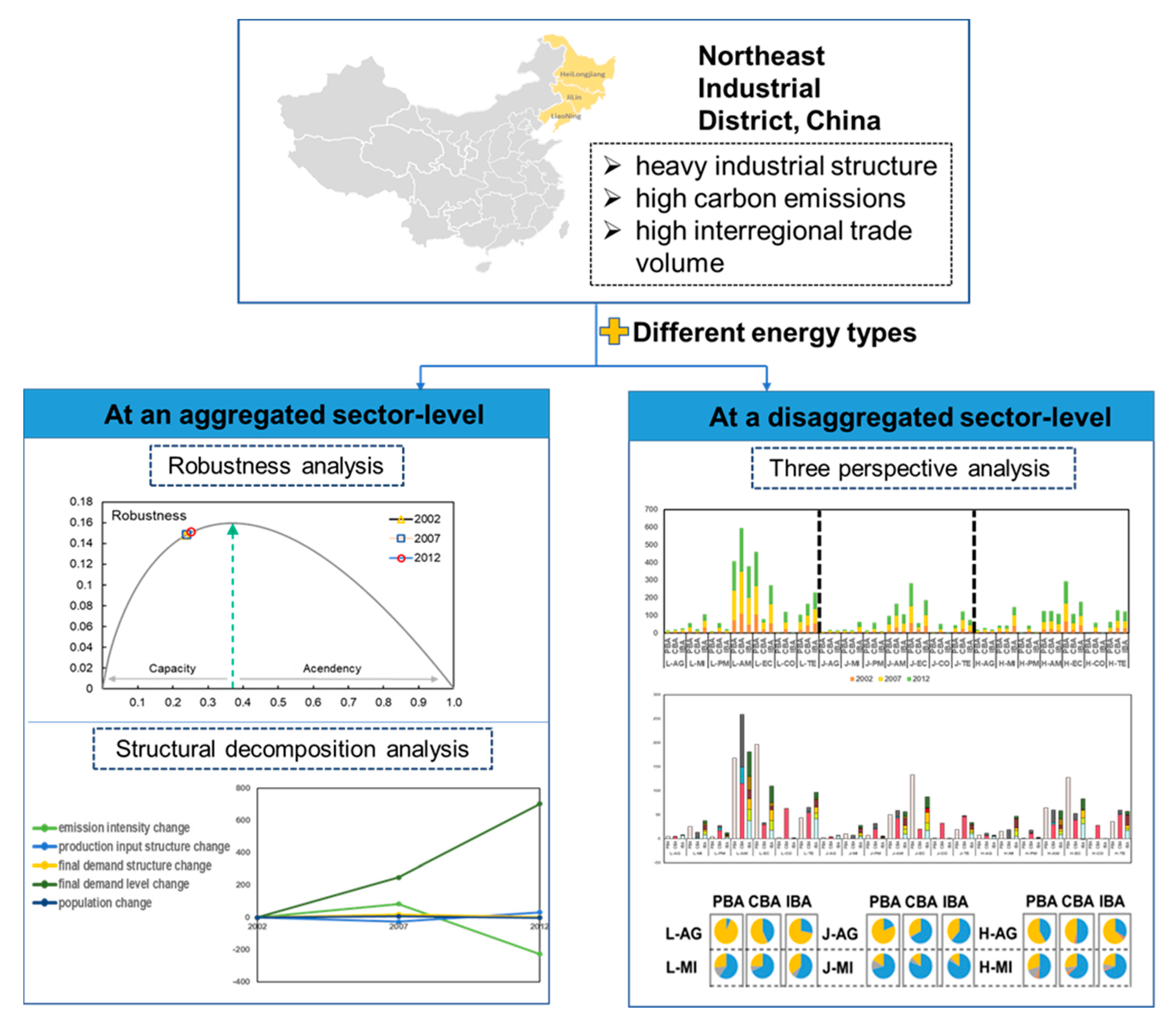
2.2. Case Study and Data Sources

The Northeast Industrial District (NID), located in the northeast of China, is the base of China’s heavy industry, covering three traditional industrial provinces: Liaoning Province (Liaoning), Jilin Province (Jilin), and Heilongjiang Province (Heilongjiang). The NID contributes significantly to China’s carbon emissions, and its GDP and carbon emission grew rapidly [28]. In 2006, the Chinese government formulated the national policy of revitalizing the old industrial base, and the NID became the fourth largest economic zone in China. However, the problems of weak economic development and environmental issues have become increasingly prominent in recent years. In detail, the NID’s carbon emissions accounted for about 11% of China’s total carbon emissions, while the GDP only accounted for 7.05% in 2016 [17]. From the perspective of the industrial structure, the NID is dominated by the secondary industry, while the secondary industry belongs to the group of high energy-consuming industries. From the perspective of the energy consumption structure, fossil fuel is the main energy source of the secondary industry, which is one of the main reasons for high carbon emissions in the NID [29]. Meanwhile, the unreasonable internal structure of the advantageous industries and the gradual migration of technical talents have led to a slow stagnation in economic development in the NID. Considering the characteristics of the heavy industrial structure, high carbon emissions, and high interregional trade volume, the NID is a typical representative of the group of regions with rapid economic and carbon emissions growth [30]. That is why the NID was selected as our case study.

There are two types of data for this research. The first data type is the carbon emission of various sectors using different energy types in the NID in 2002, 2007, and 2012, taken from the China Emission Accounts & Datasets. The second is the Multiregional Input–Output (I–O) Table for China in 2002, 2007, and 2012, which could be obtained from Liang’s research team. We choose data from 2002, 2007, and 2012 because it corresponds to the latest edition of I–O tables released in China; it includes 30 provinces, with 30 sectors in each province. We selected the data of Heilongjiang, Jilin, and Liaoning Province as the intermediate transaction’s matrix, and merged the trade exchange data between other provinces and the NID region into the flow outside the province and the flow from other provinces. Then, the multiregional I–O tables for the NID region in 2002, 2007, and 2012 could be established as important input data for the ICENM model.

2.3. Technical framework and Model Construction

In this study, an integrated carbon emission network model (ICENM) for the Northeast Industrial District (NID) is developed to quantify the relative contributions of socioeconomic factors to carbon emission changes and evaluate production-based, consumption-based, and income-based carbon emissions of different sectors. Figure 1 illustrates the technical framework and model structures for the modeling of the carbon flow network. To investigate and distinguish the impact of different energy consumption levels on carbon emissions, four representative energy groups were developed and analyzed, including coal, crude oil, natural gas, and other energy types. In detail, due to the low emissions of clean energy and the limitation of data availability, energies in other energy groups mainly include: coke, gasoline, kerosene, diesel, fuel oil, liquefied petroleum gas, heat, and electricity. Coal, crude oil, natural gas, and other energy groups refer to emissions from various industries due to consumption of these four types of energy. The first step was to explore the system’s carbon emission drivers and robustness from the perspective of the aggregated sector-level. The robustness analysis and structural decomposition analysis are based on the I–O framework. The influence of different energy types on the system’s robustness and the determination of the driving factors were studied. Furthermore, at the disaggregated level, enabled and embodied emission intensities were calculated to reveal the internal structure of the system from the production-based, consumption-based, and income-based perspectives. More specifically, emissions from specific categories of final demand and primary input were quantified. Three-perspective emissions of sectors caused by different energy types were also identified.

By combining the dynamic carbon emission data of various sectors, the ICENM model was established based on the economic I–O model framework. We treated sectors and carbon flows as nodes and paths in a network model. In detail, the I–O tables of the NID in 2002, 2007, and 2012 were divided into 21 sectors (seven distinctive sectors from three regions) according to the different social production functions of the sectors, aiming at the key sectors of the region and the more targeted calculations and analyses. The sectors include the agriculture sector (AG), mining sector (MI), primary manufacturing sector (PM), advanced manufacturing sector (AM), energy conversion and management sector (EC), construction sector (CO), tertiary sector (TE). The I–O tables for the NID including 21 sectors are listed in the Supporting Information. The embodied emission intensity and enabled emission intensity are introduced based on the Leontief inverse matrix and the Ghosh inverse matrix. Details of calculation and conversion are given in the Supplementary Materials.

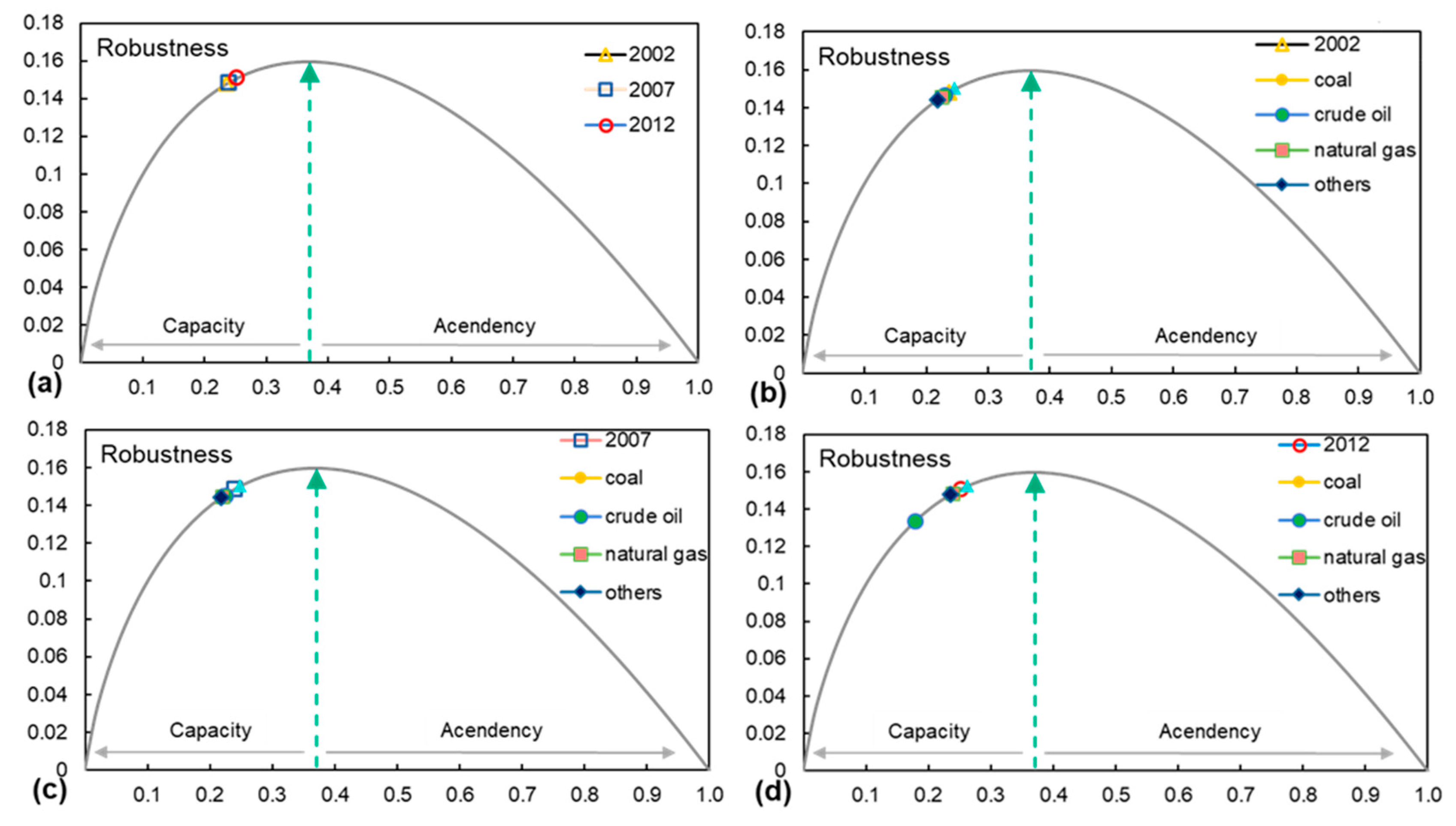
2.4. Robustness Analysis

Based on the Leontief framework, the information-based ecological network analysis (ENA), which originated from the probability theory and the graph theory, has been applied to the analysis of urban carbon emissions for holistically assessing the structure and function of the system [31,32,33,34]. The robustness analysis adopts a system-oriented paradigm to emphasize the overall characteristics of the network and explore the structure of the networked system together with energy and material flows [35]. The Identification of the system’s configuration is the key to keeping the balance between system efficiency and redundancy [36]. In detail, it combines an extensive parameter that measures the total consumption of the system to verify its robustness, thus providing a powerful tool for quantifying system sustainability [37]. The physical flow of the system could be calculated through the embodied intensity matrix:

$$\mathbf{H}=\mathsf{\epsilon }\mathbf{F}$$

(1)

where $H=[h_{ij}]$ is the physical flow matrix, and $h_{ij}$ represents the physical flow (i.e., direct emission flow) from sector $i$ to sector $j$. In a carbon emission system, there are various carbon emission pathways with different intensities [11,38]. If a system has limited pathways and each pathway has strong emission flows, the system is well organized and ordered but is also vulnerable to external interference [39]. Conversely, a system with multiple parallel circulation pathways (though some weaker and inefficiency pathways) and equally distributed emissions is more able to cope with internal and external changes when faced with disruptions [40,41]. To identify the balance status between efficiency and redundancy, the information-based ecological network analysis (i.e., robustness analysis) could be utilized for holistically analyzing the system’s efficiency and redundancy [42]. Therefore, the network’s efficiency could be expressed from the average mutual information $AMI$ from the structural perspective, and the redundancy of the system could be expressed from the residual uncertainty $H_c$:

$$\mathbf{AMI}=K{\displaystyle \sum _{i,j}{r}_{ij}}log(\frac{r_{ij}}{r_{i.}{r}_{.j}})=K{\displaystyle \sum _{i,j}\left(\frac{h_{ij}}{T_{..}}\right)}log(\frac{h_{ij}{T}_{..}}{T_{i.}{T}_{.j}})$$

(2)

$${\mathbf{H}}_{\mathbf{c}}=-K{\displaystyle \sum _{i,j}{r}_{ij}}log(\frac{1}{r_{i.}{r}_{.j}})=-K{\displaystyle \sum _{i,j}\left(\frac{h_{ij}}{T_{..}}\right)}log(\frac{h_{ij}{}^2}{T_{i.}{T}_{.j}})$$

(3)

where $r_{i.}=T_{i.}/T_{..}$, $r_{.j}=T_{.j}/T_{..}$ represent the ratio of carbon flows originating from sector $i$ to total system flow and the ratio of carbon flows streaming into sector $j$ to total system flow separately. $r_{ij}=h_{ij}/T_{..}$ shows the ratio of carbon flows descending from sector $i$ to sector $j$ to total flow. $K$ is the scale coefficient, which is determined by the base of logarithm, and $K=1$ in this study. An ICENM with a higher $AMI$ suggests that the network system is centralized and has fewer decentralized emission paths, showing that it is more organized and can provide more information. It quantifies regular, coherent, orderly, and efficient behaviors within a system. However, the tighter constraints on the movement of the medium mean that there are fewer options for parallel pathways, which may leave the ICENM in a brittle state in the face of oscillation. Thus, the indeterminate and unconfirmed part of the emission flows (i.e., the system’s residual uncertainty $H_c$) ensures the stability of the system and reduces the possibility of a system crash from an authentic structural perspective.

The proportion of development capacity (the system’s robustness) could be utilized to quantify the balance of efficiency and redundancy. The relative efficiency $a$ is a measure of the organizational flows within the system, which can be used to determine the balance between system constraints. Taking the measure of relative order and multiplying it by its disorder degree, the robustness can be reduced as $R_{ICENM}$ [43]. The order part can be measured by the relative order (i.e., $a$), and the disorder part can be derived from the Boltzmann measure (i.e., $-\mathit{alog}\left(a\right)$) [44].

$${a=\mathit{AMI}/(\mathit{AMI}+H}_c)$$

(4)

$$R_{\mathit{ICENM}}=-\mathit{alog}\left(a\right)$$

(5)

The curve of $R_{\mathit{ICENM}}$ illustrates the changes in the system’s robustness (i.e., the tradeoff relationship between system efficiency and redundancy) over time. The x-axis shows the degree of order and represents the efficiency part of the system. If the indicator lies on the left side of the curve, the ICENM tends to have less efficiency and more redundancy. On the contrary, the system is fragile as excessive efficiency leads to sacrificing redundancy, when the indicator lies on the right side of the curve.

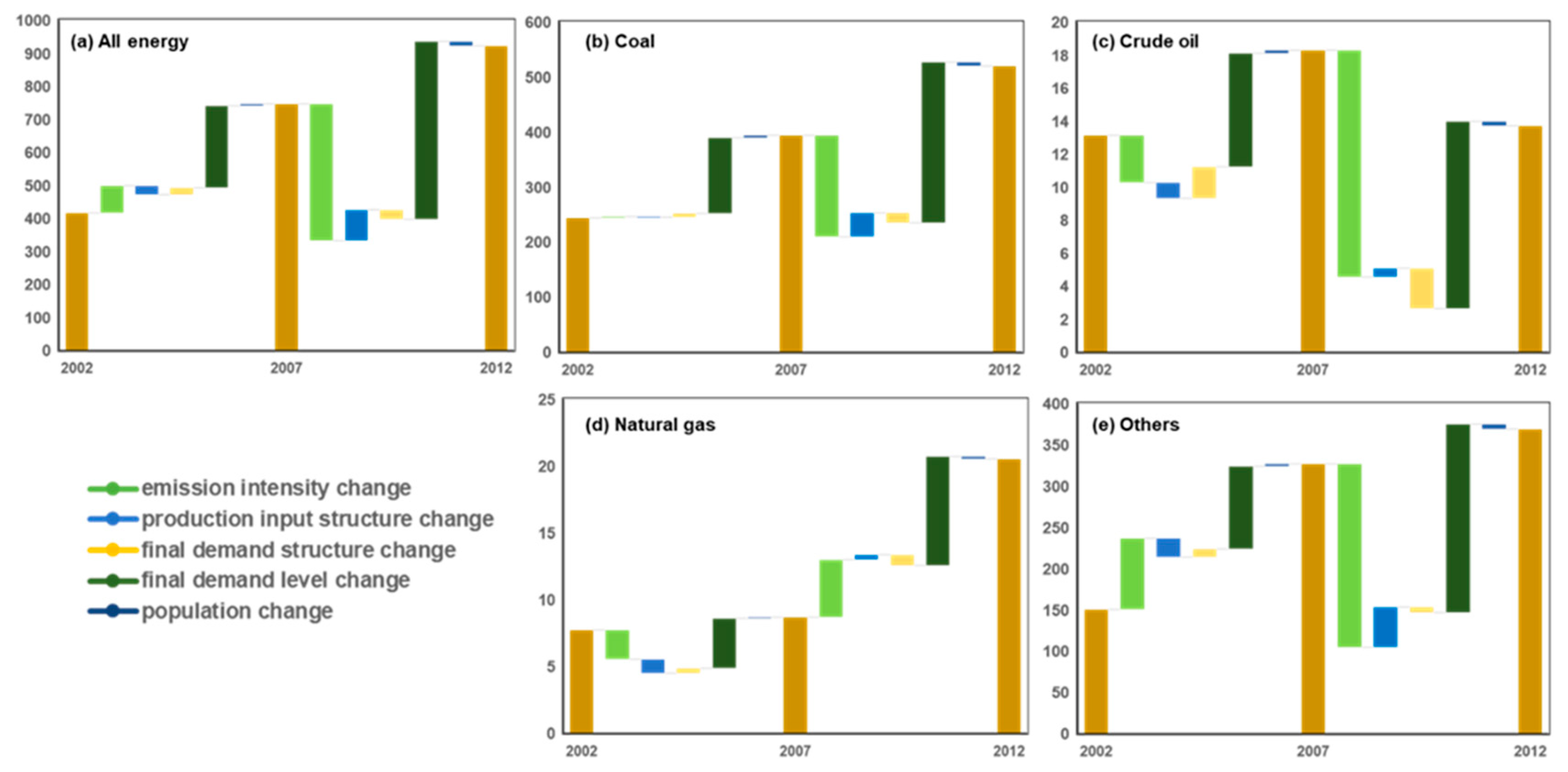
2.5. Structural Decomposition Analysis

Socioeconomic activities are viewed as the major drivers of environmental emission [45]. Regarding the research approach, the decomposition analysis (DA) is a method that establishes a model by transforming mathematical identities and decomposing the carbon emissions or emission intensity changes into certain predetermined factors to ascertain the relative impact of each factor on the total carbon dioxide emissions [46,47]. The DA methods are mainly grouped into three categories: structural decomposition analysis (SDA), index decomposition analysis (IDA), and production-theoretical decomposition analysis (PDA) [48]. The IDA is an approach that applies index theory to decomposition analysis [26,49]. It has two decomposition forms: additive decomposition and multiplicative decomposition, and requires data at only the national or industrial level [50,51]. The PDA is an approach that applies production theory to decomposition analysis. It combined the Shephard distance function and an environmental data envelopment analysis (DEA) to decompose the changes of total emissions into seven drivers. One of the advantages of the PDA is that it could reflect the impact from the perspective of technical improvement and efficiency [52]. However, the IDA and PDA methods cannot reflect structural characteristics of the economy (such as the structure of production and final demand), because the economic sectors are highly aggregated and final demand is not considered in these methods. An SDA based on an input–output framework could solve this limitation of the IDA and PDA methods [53]. SDA can facilitate decision-making at the sectoral or product scale and the allocation of responsibility for environmental impacts throughout the whole supply chain. However, the SDA has large data requirements and needs more than a one-year input–output table, and most of the countries do not prepare input–output tables every year.

To analyze the characteristics of the economic structure, we used the SDA approach to investigate relative contributions of economic factors to emission changes. Based on the Leontief framework, the carbon emissions could be decomposed as the effects of five consumption-based driving factors:

$$c=\epsilon \widehat{y}={\epsilon }^{d}L\widehat{y}={\epsilon }^{d}L{y}_s{y}_l{y}_p$$

(6)

where $c$ is the consumption-based carbon emissions; $y_{\mathrm{s}}$ indicates the final demand structure (i.e., percentage share of each sector in each category of final demand); vector $y_l$ represents the final demand level (i.e., final demand volume per capita); and $y_p$ stands for the population. The change of carbon outflow from time $t$ to time $t+1$ can be obtained through the following equations:

$$△c=△{\epsilon }^{d}L{y}_s{y}_l{y}_p+{\epsilon }^d△L{y}_s{y}_l{y}_p+{\epsilon }^{d}L△y_s{y}_l{y}_p+{\epsilon }^{d}L{y}_s△y_l{y}_p+{\epsilon }^{d}L{y}_s{y}_l△y_p$$

(7)

$$\begin{array}{l}△c={\epsilon }^d{}_{(t+1)}{L}_{(t+1)}{y}_{s_{(t+1)}}{y}_l{}_{{}_{(\mathrm{t}+1)}}{y}_{p_{(\mathrm{t}+1)}}-{\epsilon }^d{}_{(\mathrm{t})}{L}_{(t)}{y}_{s_{(t)}}{y}_l{}_{{}_{(\mathrm{t})}}{y}_{p_{(\mathrm{t})}}\\ =△{\epsilon }^d{L}_{(t)}{y}_{s_{(t)}}{y}_l{}_{{}_{(\mathrm{t})}}{y}_{p_{(\mathrm{t})}}+{\epsilon }^d{}_{(t+1)}△L{y}_{s_{(t)}}{y}_l{}_{{}_{(\mathrm{t})}}{y}_{p_{(\mathrm{t})}}+{\epsilon }^d{}_{(t+1)}{L}_{(t+1)}△y_s{y}_l{}_{{}_{(\mathrm{t})}}{y}_{p_{(\mathrm{t})}}\\ +{\epsilon }^d{}_{(t+1)}{L}_{(t+1)}{y}_{s_{(t+1)}}△y_l{y}_{p_{(\mathrm{t})}}+{\epsilon }^d{}_{(t+1)}{L}_{(t+1)}{y}_{s_{(t+1)}}{y}_l{}_{{}_{(\mathrm{t}+1)}}△y_p\end{array}$$

(8)

where Equation (7) is the additive decomposition, which analyzes the carbon emission change caused by five driving factors including emission intensity, production input structure, final demand structure, final demand level, and population. $△{\epsilon }^d$, $△L$, $△y_s$, $△y_l$, and $△y_p$ represent relative contributions of changes in emission intensity, in economic production input structure, in final demand structure, in final demand level, and in population, respectively, to emission changes of an economy $△c$.

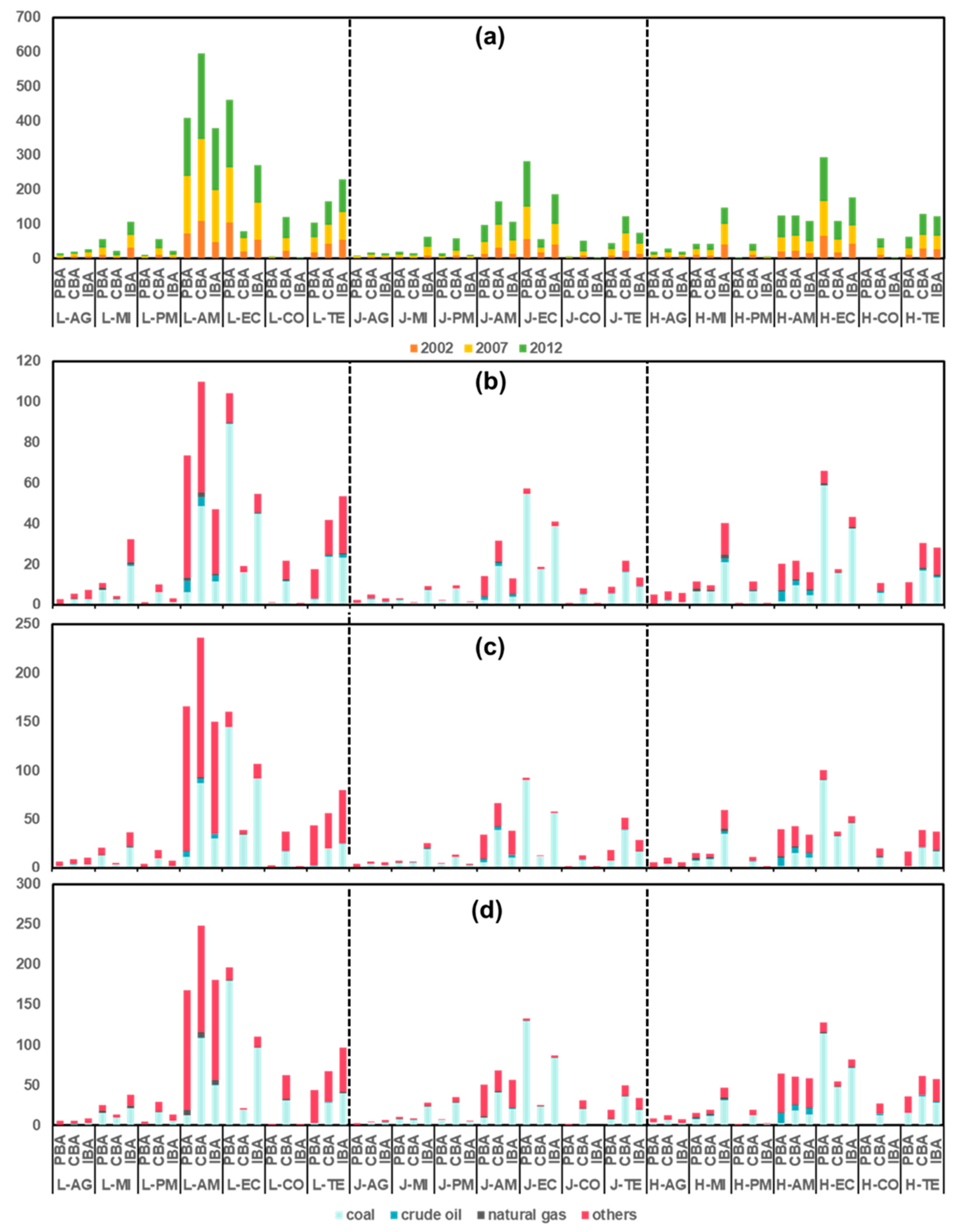
2.6. Three-Perspective Analysis

Three-perspective analysis includes production-based, consumption-based, and income-based accountings of different sectors under different types. Specifically, the production-based emissions of a sector are the direct emissions from its local production activities; the consumption-based emissions of a sector refer to the total upstream emissions (i.e., the embodied emissions) caused by its final consumption (e.g., local consumption, investment and exports final use, export and flows outside the province); the income-based emissions of a sector mean the total downstream emissions (i.e., the enabled emissions) pulled by its primary inputs (e.g., value-added, import, and flows from other provinces). The production-based ($P_i{}^p$), consumption-based ($P_i{}^c$) and income-based ($P_i{}^s$) emissions of sector $i$ are obtained by Equation (9) to Equation (11).

$$P_i^p={\epsilon }^d{}_i\times T_i$$

(9)

$$P_i^c=\epsilon L\widehat{y}={\epsilon }^d{(I-A)}^{-1}\widehat{y}$$

(10)

$$P_i^s=vG\theta =v{(I-B)}^{-1}({\epsilon }^d{)}^{\prime }$$

(11)

Furthermore, the emissions are disaggregated by final demand and primary input categories considering different energy types.

3. Results

3.1. Robustness Analysis

Figure 2a illustrates the relationship between $a$ and $R_{ICENM}$ during the study period. As shown in Figure 2a, most of the dots are on the left side of the robustness curve with less efficiency and higher redundancy, which indicates that the higher efficiency of the system is limited by the stable circulation and interaction. The highest value of $a$ and $R_{ICENM}$ of ICENM has been found in 2012, suggesting that the system in 2012 had stronger consistency, regularity, and orderliness when compared with the robustness in other years. A higher redundancy describes the flexibility that a system maintains for overcoming disturbances and shocks to its network. Figure 1b–d depict the dynamic changes of system robustness considering different emission sources. Specifically, figure b and c are not significantly affected by the energy type. Emissions from natural gas and crude oil increased the efficiency of the system in 2002 and 2007. In 2012, emissions from crude oil significantly increased the system’s redundancy and inhibited the system’s efficiency. The robustness of the system is made up of the superposition of various energy utilization effects.

3.2. Structural Decomposition Analysis

Socioeconomic factors such as population, technological progress, and structural changes will influence the change of carbon emissions. Figure 3a shows the contributions of various factors to the change of system carbon emissions. The increase in the final demand level (i.e., final demand volume for per capita) was the major driving force leading to the increase of carbon emissions during the study period. The increase of emission intensity contributed 83.5 Mt to the emission increase during 2002-2007, if other factors remained at the 2002 level; however, the reduction of emission intensity contributed 416.0 Mt to the emission reductions during 2007-2012, if other factors remained at the 2007 level. Figure 3b–e compare the contributions of various factors to the changes in system carbon emissions under different energy groups. The final demand level is the most important factor in the growth of carbon emissions under all energy groups, contributing to the growth of 405.7 Mt emissions in the coal energy group, 17.9 Mt emissions in the crude oil energy group, 14.0 Mt emissions in the natural gas energy group, and 264.4 Mt emissions in the other energy groups. The performance of the natural gas energy group is different from the contribution trend of social factors in all energy groups. In the natural gas energy group, the reduction of emission intensity contributed 2.2 Mt to the emission reductions during 2002–2007, if other factors remained at the 2002 level; however, the increase of emission intensity contributed 4.3 Mt to the emission increase during 2007–2012, if other factors remained at the 2007 level. In terms of the magnitude of emissions, the influence of coal and others groups on emission changes is the largest, and the socioeconomic factors affecting the emission changes of these two energy groups are basically consistent with the trends of all energy groups.

As shown in Figure 4, the least significant change of emissions is present in the crude oil and natural gas energy groups, which is consistent with the results found in Figure 3. Coal and others are the main types of energy that influence the changes of driving forces. Specifically, the contribution of coal energy to emission change is 30 times larger than that of natural gas. In Figure 3, in addition to the driving factor of the final demand level, the contribution of other factors to increasing emissions has changed over time. For example, the change of emission intensity has increased emissions by 83.5 Mt from 2002 to 2007, and reduced emissions by 416.0 Mt from 2007 to 2012. Thus, for each driving factor, attention must be paid to the energy types that have a positive impact on the driving factor reducing the emission, and the energy types that have a negative effect on the driving factor increasing emissions. The final demand level is not sensitive to the change of energy types because all energy sources have a positive effect on them. Other drivers respond differently to different energy types in different periods. In detail, from 2007 to 2012, the emission intensity has decreased 416.0 Mt, while under the natural gas energy group, the emission intensity has increased 4.3 Mt in the natural gas energy group. This shows that the natural gas utilization intensity of the system is not high and needs to be improved.

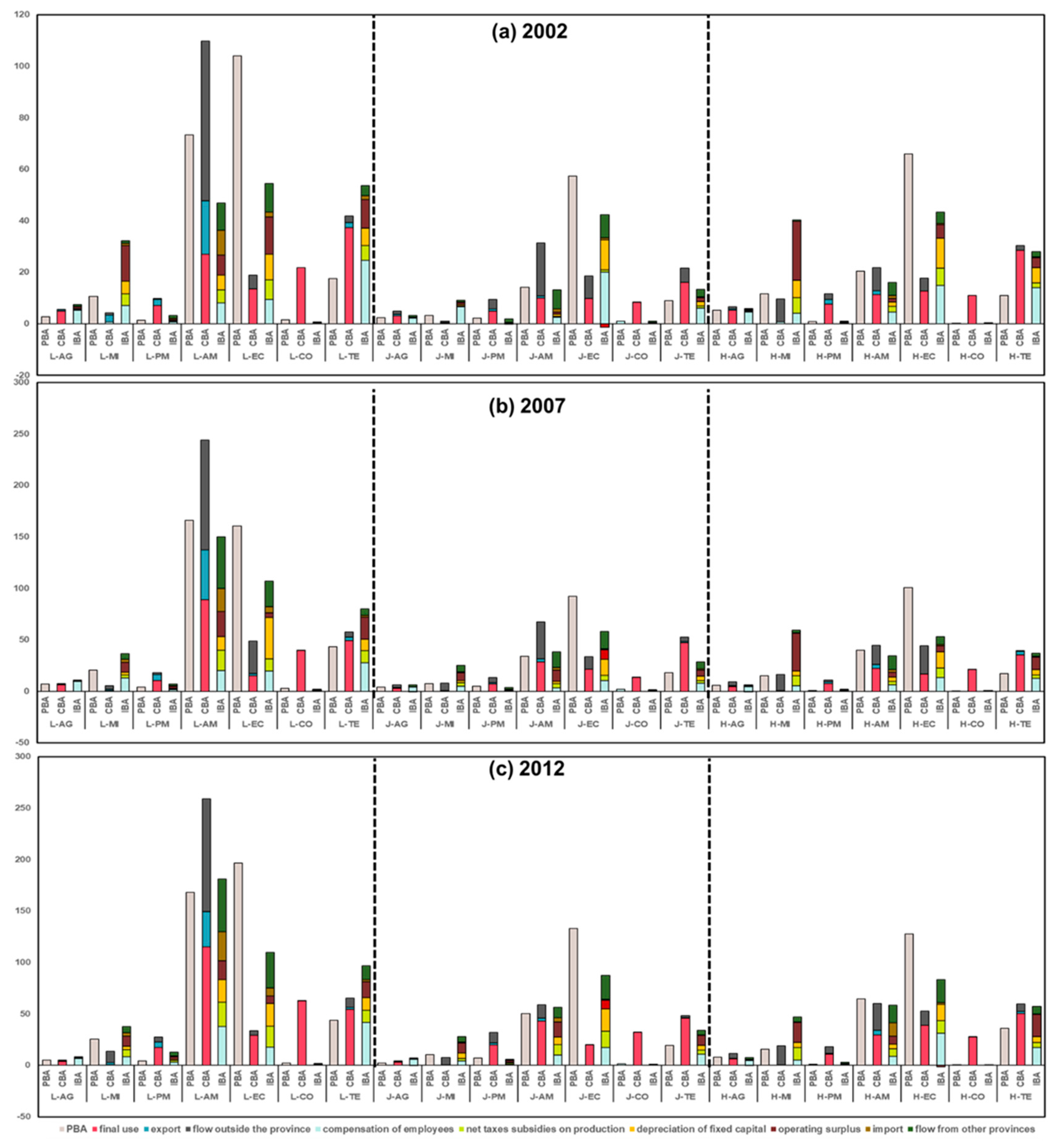
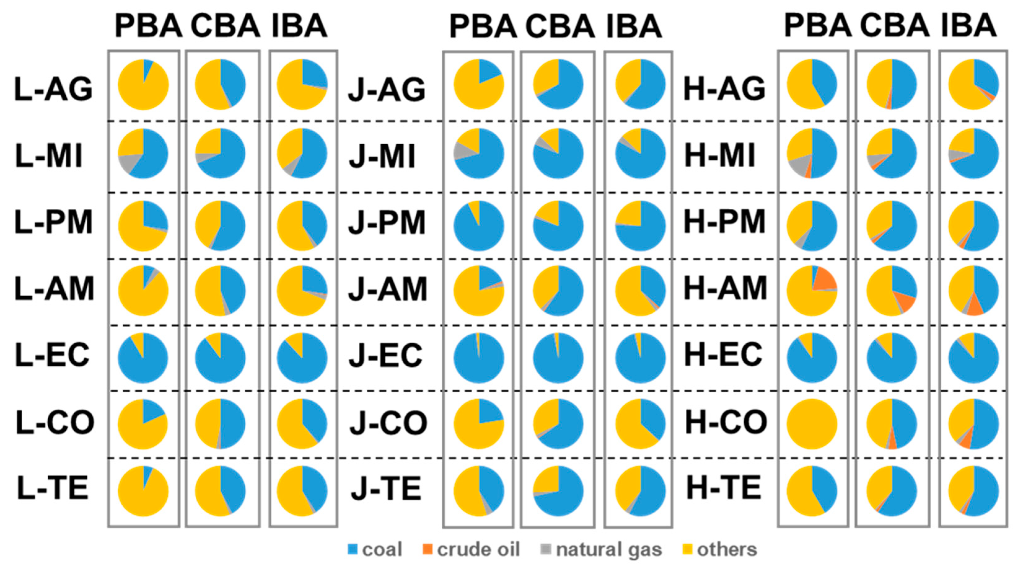
3.3. Three Perspective Analysis

Figure 5a accounts for cumulative production-based, consumption-based, and income-based emissions of different sectors during the study period. It could be seen from Figure 5a that L-AM has the largest cumulative consumption-based emissions, 594.32 Mt, followed by L-EC’s cumulative production-based emissions, 461.3 Mt. For Heilongjiang and Jilin, the cumulative emissions of the highest cumulative emissions are J-EC’s production-based emissions, of 282.7 Mt, followed by J-EC’s income-based emissions, of 186.3 Mt. For Heilongjiang, the cumulative emissions of H-EC are the largest production-based emissions, followed by the income-based emissions of H-EC. The emission accountings of each sector from different perspectives basically show a year-by-year growth trend. In terms of different sectors, the main production-based sectors are L-EC, J-EC, H-EC, while the main consumption-based sectors are L-AM, L-CO, J-PM, J-CO, J-TE and H-CO, and the income-based sectors are L-MI, L-TE and H-MI. Comparing Figure 5a–c, it is found that no matter which type of energy causes the emission, the emission accounting values obviously increase with the year. The contribution of different energy sources to emissions is roughly the same during the study period. In detail, for AM including the L-AM, J-AM, and H-AM sectors, coal’s contribution to their production-based emissions is greater than that of consumption-based and income-based emissions. The production-based emissions from the L-TE sector are mainly caused by the usage of coal. The emissions from three perspectives of EC (i.e., the L-EC, J-EC, and H-EC sectors) are mainly caused by the usage of other energy sources.

Figure 6 further disaggregates the emissions of different sectors by final demand and primary input categories over time. There are three categories of final demand, including final use (FU), export (EX), and flow outside the province (FOTP). There are six categories of primary input, including compensation of employees (CE), net taxed subsidies on production (NTS), depreciation of fixed capital (DFC), operating surplus (OS), import (IM), and flow from other provinces (FFOP). Overall, the change in emissions caused by different categories over time is not significant. Take 2012 as an example: on the final demand side (i.e., consumption-based perspective), FU is the major driver, contributing 66.5% to carbon emissions in 2012. In detail, FU contributes more than 99.6% of carbon emissions to the J-CO, L-CO and H-CO sectors. In addition, the FU contributes more than 90% to the emissions of L-TE, J-TE, and C-TE. For L-AM, FOTP (42.3%) and final use (44.5%) are the main contributions. On the primary supply side (i.e., income-based perspective), CE is the main enabler, which leads to a total of 25.2% of carbon emissions. Specifically, CE contributes 82.5%, 86%, and 65.6% to the L-AG, J-AG, and H-AG sectors, which shows that the IBA emissions of the AG sector in the system mainly come from the contribution of CE. For L-EC, L-CO, H-PM, and H-CO, the contribution of FFOP to emissions is more than 30%. Comparing Figure 4a–c, it can be found that although the magnitude of emissions is increasing, the contribution of different categories to emissions in various sectors has generally changed little. Among them, the PBA emissions of L-AG, L-CO, J-AG, and J-CO reached their peak in 2007 and began to decrease in 2012; however, the emissions of other sectors are increasing year by year, but there is a gap in the growth rate of each sector. The emission growth rate of some sectors in Liaoning has slowed down. For example, the growth rate changed from 126.5% to 1.1% for L-AM. The growth rate of sectors in Jilin has been reduced by about half. As for most sectors in Heilongjiang, the slowdown trend in growth rate is relatively low. From a consumption-based perspective, FOTP’s contribution to L-MI’s emissions increased year by year, accounting for 17.0%, 57.2%, and 75.6% respectively; however, the contribution of FTOP to J-EC decreased during the study period. From an income-based perspective, the proportion of FFOP’s contribution to emissions increased by 14.7%, 23.5%, and 31.4% in 2002, 2007, and 2012. In general, it could be found that 2002 is a turning year; the structural change in 2007 was relatively large, and emissions were reduced.

Figure 7 focuses on the contribution difference of different energy types to three-perspective emissions for each sector. Overall, coal and others energy types are the main contributions to the emissions. From the vertical perspective, the emission differences among provinces could be compared, and it was found that the emission accountings of L-EC for various energy types in Liaoning are basically insensitive to the impact of the accounting perspectives. From a production-based perspective, others contributed the most to the L-AG, L-AM, and L-TE sectors, and coal contributed the most to the remaining sectors. Moreover, coal was the largest source of the consumption-based emissions for the L-MI, L-PM, L-EC, and L-TE sectors; and others contributed the most to the emissions of other sectors. For Jilin, the emissions of J-PM, J-EC, J-CO, and J-MI from different energy types were basically not affected by the accounting perspectives. For Heilongjiang, the production-based emissions of H-AG and H-TE were mainly caused by others, accounting for about 90%. From a horizontal perspective, the three-perspective emissions of the EC sectors in each province were not affected by the energy type. The contribution of coal was relatively large, ranging from 87.8% to 98.0%.

4. Discussion

In this research, an integrated carbon emission network model (ICENM) has been developed and applied to the Northeast Industrial District (NID), China, to investigate the driving forces of carbon emission changes and construct carbon emission inventories at the aggregated and disaggregated sectoral levels. In detail, different emissions from different energy types, including coal, crude oil, natural gas, and other energy groups, were considered. Under the input–output framework of this study, an SDA has been used to explore the relative contribution of socioeconomic factors to carbon emission changes in the NID from 2002 to 2012 at an aggregated sectoral level. The system’s efficiency, redundancy, and robustness have been evaluated to comprehensively diagnose its health condition and provide recommendations for its sustainable development. Furthermore, direct, enabled, and embodied emission intensities have been calculated to investigate the changes in production-based, consumption-based, and income-based emissions inventories in various sectors at a disaggregated sectoral level. Emissions from detailed categories of final demand and primary inputs are quantified to guide specific emission measures. The current study could provide empirical evidence for guiding the formulation of the NID’s regional emission reduction policies, to ensure a more balanced and sustainable system.

China will continue to pursue a higher quality of life, which will lead to a higher final demand level. Therefore, the increase of the final demand level in the future will proceed to push up carbon emissions in the NID. On the other hand, the NID could take action in the following directions to reduce its carbon emissions: carbon emission intensity and production input structure. Firstly, reducing the intensity of the industry’s carbon emissions is conducive to a decrease in carbon emissions. Measures involve shifting the energy mix from coal to less carbon-intensive energy sources (e.g., natural gas and nuclear power), upgrading energy utilization efficiency, and employing carbon capture and storage (CCS) technologies. In particular, special attention should be paid to natural gas energy utilization efficiency in the NID region. Moreover, these actions should be mainly focused on key sectors with large production-based emissions, such as the energy conversion and management sector in three provinces (Figure 3a). Secondly, changing the production structure also contributes to reducing emissions. It is found that the change of production structure tends to increase carbon emissions. Production input structure expresses the total upstream inputs required to produce unitary finally-used products, denoting the production efficiency of each sector. Improving sectoral productivity (i.e., producing the same output with less upstream inputs) could help reduce emissions for the upstream sectors. This action should be mainly focused on key sectors with large consumption-based emissions, such as the primary manufacturing sector and the advanced manufacturing sector of three provinces in the NID region (Figure 3a). Thirdly, the impact of changes in the final demand structure on carbon emission reductions remain relatively stable, suggesting that there may be great potential to change the final demand structure for carbon emission reductions in the NID. Final use and flow outside the province are the dominant final demand categories leading to carbon emissions in the NID (Figure 4). Accordingly, changing household consumption behaviors (e.g., encouraging consumers to use products with less carbon-intensive components through a life cycle eco-label certification and economic means) are conducive to reducing the NID’s carbon emissions, especially household consumption behaviors regarding products from the tertiary sectors of the three provinces (Figure 4). Moreover, it is of great importance to improve the commodity trade modes between the NID and other provinces. Through the coordinated development among provinces, strengthening the product demand of other regions for the NID (e.g., requiring the NID to sell less carbon-intensive products), especially for products from advanced the manufacturing sector in Liaoning.

In addition to the amount of emissions, the current policies should also focus on the system’s long-term sustainability (i.e., the balance between efficiency and redundancy for emission circulation). The system’s robustness results show that the index is a comprehensive evaluation index reflecting the balance between the system’s efficiency and redundancy. As shown in Fig. 1, one robustness value (i.e., the value of R_ICENM) corresponds to two values that fall into different regions, respectively. Though the robustness of the system is the same, the state of the system is the opposite. A value of robustness close to the highest point of the curve indicates that the system has both high efficiency and high redundancy. If the R_ICENM point falls on the left side of the curve, there are too many repetitive and inefficient paths flowing in the system. Conversely, the points on the right side of the curve indicate that the pursuit of efficiency is achieved at the expense of the necessary stability, and the circuitous paths may lead to the overall performance being too fragile to cope with internal and external changes, such as the turbulence of the economic structure. For the NID, the carbon emission system has high redundancy and low efficiency, indicating that there are many emission pathways within the system. Moreover, the use of crude oil significantly increases system redundancy and inhibits system efficiency. This is mainly because the production capacity of crude oil in the NID is decreasing, but crude oil consumption is increasing. Thus, the exploration of oil resources should be strengthened, to improve the regional security capacity. On the other hand, it is very important to deepen the cooperation with Northeast Asia, to improve the security capabilities from outside the region. Simultaneously, different policies or regulations should be adopted to achieve carbon reductions in different sectors, to coordinate the intensification and scale of the petrochemical industry by shrinking costs and improving efficiency, and thereby reducing oil consumption in the NID region.

5. Conclusions

This paper develops an ICENM model for the NID at the aggregated and disaggregated levels to facilitate the development of an integrated carbon mitigation policy. The paper fills a gap in the literature, given the very limited studies on comprehensive urban agglomeration carbon analysis. It is found that the increase of the final demand level will proceed to push up carbon emissions in the NID. However, the NID could take action from the perspective of carbon emission intensity and production input structure to reduce its carbon emissions. Moreover, a change in the production structure tends to increase carbon emissions. It is of great importance to improve the commodity trade modes between the NID and other provinces. As for the choices of different energy types, the use of crude oil significantly increases system redundancy and inhibits system efficiency.

A significant difference between our research and the previous research is the emphasis on the integrity of the system, that is, the system is evaluated from the perspective of aggregated and disaggregated sectoral levels. It is also worth mentioning that the NID is representative of regions with a heavy industrial structure and high carbon emissions. The general observations of this study also have some reference value for other regions with similar characteristics, such as Detroit, USA, and Ruhr, Germany. Moreover, the methodology developed by this research has implications for exploring carbon emissions in any region of the world. However, some limitations will be addressed in future research. First, longer-term changes of the system should be considered, while only three-year changes of the system are analyzed due to the timing of input–output analysis. Thus, in future research, some methods that are not based on an input–output framework could be considered, such as IDA. Second, emission reduction simulation, considering the actual policies, is of great necessity to reflect the rationality of policy making. Therefore, the simulations could be considered, in the future, from three perspectives, and the response of the system could be explored through different degrees of interference. Third, the cost of emission reduction policies is very important when reflecting on the economic impacts of different policies. Future research should consider how to combine regional emissions and emission reduction costs to achieve co-benefits of emission reduction and economy.

References

1. Qu, S.; Liang, S.; Xu, M. CO2 Emissions Embodied in Interprovincial Electricity Transmissions in China. Environ. Sci. Technol. 2017, 51, 10893–10902. [Google Scholar] [CrossRef]
2. Ahmad, S.; Baiocchi, G.; Creutzig, F. CO2 Emissions from Direct Energy Use of Urban Households in India. Environ. Sci. Technol. 2015, 49, 11312–11320. [Google Scholar] [CrossRef]
3. Zhai, M.; Huang, G.; Liu, L.; Zhang, X. Ecological network analysis of an energy metabolism system based on input-output tables: Model development and case study for Guangdong. J. Clean. Prod. 2019, 227, 434–446. [Google Scholar] [CrossRef]
4. Zhai, M.; Huang, G.; Liu, L.; Su, S. Dynamic input-output analysis for energy metabolism system in the Province of Guangdong. China. J. Clean. Prod. 2018, 196, 747–762. [Google Scholar] [CrossRef]
5. Wang, S.; Chen, B. Energy–water nexus of urban agglomeration based on multiregional input–output tables and ecological network analysis: A case study of the Beijing–Tianjin–Hebei region. Appl. Energy 2016, 178, 773–783. [Google Scholar] [CrossRef]
6. Zhang, Y.; Zheng, H.; Yang, Z.; Li, Y.; Liu, G.; Su, M.; Yin, X. Urban energy flow processes in the Beijing-Tianjin-Hebei (Jing-Jin-Ji) urban agglomeration: Combining multi-regional input-output tables with ecological network analysis. J. Clean. Prod. 2016, 114, 243–256. [Google Scholar] [CrossRef]
7. Zhai, M.; Huang, G.; Liu, H.; Liu, L.; He, C.; Liu, Z. Three-perspective energy-carbon nexus analysis for developing China’s policies of CO2-emission mitigation. Sci. Total Environ. 2020, 705, 135857. [Google Scholar] [CrossRef]
8. Zhang, Y.; Yang, Z.; Yu, X. Urban Metabolism: A Review of Current Knowledge and Directions for Future Study. Environ. Sci. Technol. 2015, 49, 11247–11263. [Google Scholar] [CrossRef]
9. Zhang, Y. Urban metabolism: A review of research methodologies. Environ. Pollut. 2013, 178, 463–473. [Google Scholar] [CrossRef]
10. Chen, S.; Chen, B. Changing Urban Carbon Metabolism over Time: Historical Trajectory and Future Pathway. Environ. Sci. Technol. 2017, 51, 7560–7571. [Google Scholar] [CrossRef]
11. Chen, L.; Xu, L.; Yang, Z. Accounting carbon emission changes under regional industrial transfer in an urban agglomeration in China’s Pearl River Delta. J. Clean. Prod. 2017, 167, 110–119. [Google Scholar] [CrossRef]
12. Song, J.; Feng, Q.; Wang, X.; Fu, H.; Jiang, W.; Chen, B. Spatial association and effect evaluation of CO2 emission in the Chengdu-Chongqing urban agglomeration: Quantitative evidence from social network analysis. Sustainability 2018, 11, 1. [Google Scholar] [CrossRef] [Green Version]
13. Zhang, D.; Huang, Q.; He, C.; Wu, J. Impacts of urban expansion on ecosystem services in the Beijing-Tianjin-Hebei urban agglomeration, China: A scenario analysis based on the Shared Socioeconomic Pathways. Resour. Conserv. Recycl. 2017, 125, 115–130. [Google Scholar] [CrossRef]
14. Han, F.; Xie, R.; Lu, Y.; Fang, J.; Liu, Y. The effects of urban agglomeration economies on carbon emissions: Evidence from Chinese cities. J. Clean. Prod. 2018, 172, 1096–1110. [Google Scholar] [CrossRef]
15. Zheng, H.; Fath, B.D.; Zhang, Y. An Urban Metabolism and Carbon Footprint Analysis of the Jing–Jin–Ji Regional Agglomeration. J. Ind. Ecol. 2017, 21, 166–179. [Google Scholar] [CrossRef]
16. Kitamura, Y.; Ichisugi, Y.; Karkour, S.; Itsubo, N. Carbon Footprint Evaluation based on Tourist Consumption toward Sustainable Tourism in Japan. Sustainability 2020, 12, 2219. [Google Scholar] [CrossRef] [Green Version]
17. Cheng, H.; Dong, S.; Li, F.; Yang, Y.; Li, S.; Li, Y. Multiregional Input-Output Analysis of Spatial-Temporal Evolution Driving Force for Carbon Emissions Embodied in Interprovincial Trade and Optimization Policies: Case Study of Northeast Industrial District in China. Environ. Sci. Technol. 2018, 52, 346–358. [Google Scholar] [CrossRef]
18. Zhai, M.; Huang, G.; Liu, L.; Zheng, B.; Guan, Y. Inter-regional carbon flows embodied in electricity transmission: Network simulation for energy-carbon nexus. Renew. Sustain. Energy Rev. 2020, 118, 109511. [Google Scholar] [CrossRef]
19. Davis, S.J.; Caldeira, K. Consumption-based accounting of CO2 emissions. Proc. Natl. Acad. Sci. USA 2010, 107, 5687–5692. [Google Scholar] [CrossRef] [Green Version]
20. Chen, Z.M.; Ohshita, S.; Lenzen, M.; Wiedmann, T.; Jiborn, M.; Chen, B.; Lester, L.; Guan, D.; Meng, J.; Xu, S.; et al. Consumption-based greenhouse gas emissions accounting with capital stock change highlights dynamics of fast-developing countries. Nat. Commun. 2018, 9, 1–9. [Google Scholar] [CrossRef]
21. Marques, A. Income-based environmental responsibility. Ecological Economics 2006, 84, 57–65. [Google Scholar] [CrossRef]
22. Liang, S.; Qu, S.; Zhu, Z.; Guan, D.; Xu, M. Income-Based Greenhouse Gas Emissions of Nations. Environ. Sci. Technol. 2017, 51, 346–355. [Google Scholar] [CrossRef] [PubMed] [Green Version]
23. Chen, W.; Lei, Y.; Feng, K.; Wu, S.; Li, L. Provincial emission accounting for CO2 mitigation in China: Insights from production, consumption and income perspectives. Appl. Energy 2019, 255, 113754. [Google Scholar] [CrossRef]
24. Wang, C.; Ghadimi, P.; Lim, M.K.; Tseng, M.L. A literature review of sustainable consumption and production: A comparative analysis in developed and developing economies. J. Clean. Prod. 2019, 206, 741–754. [Google Scholar] [CrossRef]
25. Wei, J.; Huang, K.; Yang, S.; Li, Y.; Hu, T.; Zhang, Y. Driving forces analysis of energy-related carbon dioxide (CO2) emissions in Beijing: An input–output structural decomposition analysis. J. Clean. Prod. 2017, 163, 58–68. [Google Scholar] [CrossRef]
26. Liang, S.; Xu, M.; Liu, Z.; Suh, S.; Zhang, T. Socioeconomic drivers of mercury emissions in China from 1992 to 2007. Environ. Sci. Technol. 2013, 47, 3234–3240. [Google Scholar] [CrossRef]
27. Xu, X.Y.; Ang, B.W. Index decomposition analysis applied to CO2 emission studies. Ecol. Econ. 2013, 93, 313–329. [Google Scholar] [CrossRef]
28. Li, X.; Liu, L.; Wang, Y.; Luo, G.; Chen, X.; Yang, X.; Hall, M.H.P.; Guo, R.; Wang, H.; Cui, J.; et al. Heavy metal contamination of urban soil in an old industrial city (Shenyang) in Northeast China. Geoderma 2013, 192, 50–58. [Google Scholar] [CrossRef]
29. Qing, X.; Yutong, Z.; Shenggao, L. Assessment of heavy metal pollution and human health risk in urban soils of steel industrial city (Anshan), Liaoning, Northeast China. Ecotoxicol. Environ. Saf. 2015, 120, 377–385. [Google Scholar] [CrossRef]
30. Zhai, M.; Huang, G.; Liu, L.; Zheng, B.; Guan, Y. Network analysis of different types of food flows: Establishing the interaction between food flows and economic flows. Resour. Conserv. Recycl. 2019, 143, 143–153. [Google Scholar] [CrossRef]
31. Chen, Z.M.; Chen, G.Q.; Zhou, J.B.; Jiang, M.M.; Chen, B. Ecological input-output modeling for embodied resources and emissions in Chinese economy 2005. Commun. Nonlinear Sci. Numer. Simul. 2010, 15, 1942–1965. [Google Scholar] [CrossRef]
32. Tan, L.M.; Arbabi, H.; Li, Q.; Sheng, Y.; Densley Tingley, D.; Mayfield, M.; Coca, D. Ecological network analysis on intra-city metabolism of functional urban areas in England and Wales. Resour. Conserv. Recycl. 2018, 138, 172–182. [Google Scholar] [CrossRef]
33. Zhang, Y.; Yang, Z.; Fath, B.D. Ecological network analysis of an urban water metabolic system: Model development, and a case study for Beijing. Sci. Total Environ. 2010, 408, 4702–4711. [Google Scholar] [CrossRef] [PubMed]
34. Lu, Y.; Chen, B.; Feng, K.; Hubacek, K. Ecological Network Analysis for Carbon Metabolism of Eco-industrial Parks: A Case Study of a Typical Eco-industrial Park in Beijing. Environ. Sci. Technol. 2015, 49, 7254–7264. [Google Scholar] [CrossRef]
35. Goerner, S.J.; Lietaer, B.; Ulanowicz, R.E. Quantifying economic sustainability: Implications for free-enterprise theory, policy and practice. Ecol. Econ. 2009, 69, 76–81. [Google Scholar] [CrossRef]
36. Goldstein, B.; Birkved, M.; Quitzau, M.B.; Hauschild, M. Quantification of urban metabolism through coupling with the life cycle assessment framework: Concept development and case study. Environ. Res. Lett. 2013, 8, 035024. [Google Scholar] [CrossRef]
37. Li, Y.; Yang, Z.F. Quantifying the sustainability of water use systems: Calculating the balance between network efficiency and resilience. Ecol. Modell. 2011, 222, 1771–1780. [Google Scholar] [CrossRef]
38. Guan, D.; Hubacek, K.; Weber, C.L.; Peters, G.P.; Reiner, D.M. The drivers of Chinese CO2 emissions from 1980 to 2030. Glob. Environ. Chang. 2008, 18, 626–634. [Google Scholar] [CrossRef] [Green Version]
39. Chen, S.; Chen, B.; Chen, S.; Chen, B. Network Environ Perspective for Urban Metabolism and Carbon Emissions: A Case Study of Vienna. Environ. Sci. Technol. 2014, 46, 4498–4506. [Google Scholar]
40. Chen, S.; Fath, B.D.; Chen, B. Information-based Network Environ Analysis: A system perspective for ecological risk assessment. Ecol. Indic. 2011, 11, 1664–1672. [Google Scholar] [CrossRef]
41. Chen, S.; Chen, B. Urban energy consumption: Different insights from energy flow analysis, input-output analysis and ecological network analysis. Appl. Energy 2015, 138, 99–107. [Google Scholar] [CrossRef]
42. Mao, X.; Wei, X.; Yuan, D.; Jin, Y.; Jin, X. An ecological-network-analysis based perspective on the biological control of algal blooms in Ulansuhai Lake, China. Ecol. Modell. 2018, 386, 11–19. [Google Scholar] [CrossRef]
43. Ulanowicz, R.E.; Holt, R.D.; Barfield, M. Limits on ecosystem trophic complexity: Insights from ecological network analysis. Ecol. Lett. 2014, 17, 127–136. [Google Scholar] [CrossRef]
44. Boltzmann, L. Weitere studien über das wärmegleichgewicht unter gasmolekülen. In Kinetische Theorie II; Vieweg+ Teubner Verlag: Wiesbaden, Germany, 1970. [Google Scholar]
45. Xia, X.H.; Hu, Y.; Alsaedi, A.; Hayat, T.; Wu, X.D.; Chen, G.Q. Structure decomposition analysis for energy-related GHG emission in Beijing: Urban metabolism and hierarchical structure. Ecol. Inform. 2015, 26, 60–69. [Google Scholar] [CrossRef]
46. Peng, J.; Zhang, Y.; Xie, R.; Liu, Y. Analysis of driving factors on China’s air pollution emissions from the view of critical supply chains. J. Clean. Prod. 2018, 203, 197–209. [Google Scholar] [CrossRef]
47. Fan, J.L.; Da, Y.B.; Wan, S.L.; Zhang, M.; Cao, Z.; Wang, Y.; Zhang, X. Determinants of carbon emissions in ‘Belt and Road initiative’ countries: A production technology perspective. Appl. Energy 2019, 239, 268–279. [Google Scholar] [CrossRef]
48. Su, B.; Ang, B.W. Structural decomposition analysis applied to energy and emissions: Some methodological developments. Energy Econ. 2012, 34, 177–188. [Google Scholar] [CrossRef]
49. Liang, S.; Wang, H.; Qu, S.; Feng, T.; Guan, D.; Fang, H.; Xu, M. Socioeconomic Drivers of Greenhouse Gas Emissions in the United States. Environ. Sci. Technol. 2016, 50, 7535–7545. [Google Scholar] [CrossRef] [Green Version]
50. Chen, G.; Hou, F.; Chang, K.; Zhai, Y.; Du, Y. Driving factors of electric carbon productivity change based on regional and sectoral dimensions in China. J. Clean. Prod. 2020, 205, 477–487. [Google Scholar] [CrossRef]
51. Zhong, Z.; Jiang, L.; Zhou, P. Transnational transfer of carbon emissions embodied in trade: Characteristics and determinants from a spatial perspective. Energy 2018, 147, 858–875. [Google Scholar] [CrossRef]
52. Čuček, L.; Klemeš, J.J.; Kravanja, Z. A review of footprint analysis tools for monitoring impacts on sustainability. J. Clean. Prod. 2012, 34, 9–20. [Google Scholar] [CrossRef]
53. Xia, L.; Fath, B.D.; Scharler, U.M.; Zhang, Y. Spatial variation in the ecological relationships among the components of Beijing’s carbon metabolic system. Sci. Total Environ. 2016, 544, 103–113. [Google Scholar] [CrossRef] [PubMed]
Figure 1. Technical framework and model construction. Note: China map is a schematic diagram.
Sustainability 12 02708 g001
Figure 2. Relationship between a and R I C E N M in the integrated carbon emission network model (ICENM). (a) Dynamic changes of robustness in 2002, 2007 and 2012; (b) Robustness changes in different energy types in 2002; (c) Robustness changes in different energy types in 2007; (d) Robustness changes in different energy types in 2012. Note: a and R I C E N M denote the relative order and the system’s robustness (the disorder part), respectively.
Sustainability 12 02708 g002
Figure 3. Relative contributions of socioeconomic factors to the carbon emission changes of the NID region during 2002–2012. The baseline year is 2002. The unit of the Y-axis is Mt and of the X-axis is years.
Sustainability 12 02708 g003
Figure 4. Relative contributions of socioeconomic factors to the carbon emission changes during 2002–2012 considering different energy types. The unit of Y-axis is Mt and of X-axis is years.
Sustainability 12 02708 g004
Figure 5. (a) Cumulative production-based, consumption-based, and income-based carbon emissions of different sectors in 2002, 2007, and 2012; Production-based, consumption-based, and income-based carbon emissions of different sectors considering different energy sources (b) in 2002, (c) in 2007, and (d) in 2012. Note: The X-axis represents different sectors, and the unit of the Y-axis is Mt. L, J, and H represent Liaoning, Jilin, and Heilongjiang provinces.
Sustainability 12 02708 g005
Figure 6. Production-based, consumption-based, and income-based carbon emissions of different sectors in different final demand and primary input categories in (a) 2002, (b) 2007, and (c) 2012. Note: The X-axis represents different sectors, and the unit of the Y-axis is Mt. L, J, and H represent Liaoning, Jilin, and Heilongjiang provinces.
Sustainability 12 02708 g006
Figure 7. Contributions of four energy types to production-based, consumption-based, and income-based emissions for each sector in 2012. Note: L, J, and H represent Liaoning, Jilin and Heilongjiang provinces.
Sustainability 12 02708 g007