2. Literature Review
Rail transport is rapidly becoming digitalized, with an increasing role of digital technology in all aspects of the rail sector. The digital revolution is opening up many opportunities for railway operators and infrastructure manager. The digital transformation of rail systems makes it possible to increase the sustainability of asset management thanks to the introduction of decision support tools, able to exploit data from the field in order to optimize the use of resources, reducing assets’ life cycle costs (LCC). The importance of pursuing sustainability goals in railway asset management is highlighted by many works in the literature [
3,
4,
5,
6,
7].
In particular, the applied maintenance strategy may have a significant impact on life cycle cost, since poor maintenance processes imply downtimes and consequent costs.
In many sectors, a preventive approach to maintenance has become key for achieving the sustainability targets, such as in Industry 4.0 [
8], in the asset management of civil infrastructure [
9] and linear assets [
10], such as roads and bridges [
11].
In the rail sector, works deal with the introduction of sustainability concepts in asset management, applying a whole-system life cost analysis [
12,
13,
14].
To do this, multi-criteria decision analysis frameworks that incorporate sustainability criteria over the whole life cycle have been developed in the literature [
15], considering different rail assets, such as rail signaling and control systems [
16].
The possibility of receiving data in real-time, from automatic and fully integrated monitoring systems, makes it possible to develop a more sustainable and digitally supported asset management [
17,
18]. Moreover, a context-aware decision-making can be achieved, providing infrastructure operators, system suppliers, and construction companies with comprehensive information. Finally, with the introduction of Internet of Things (IoT) sensors, some assets are becoming able to perform self-diagnostics and even self-repairing [
19,
20].
In an eMaintenance context, IoT devices and smart sensors perform condition monitoring, collecting data to be used by machine learning algorithms, to achieve predictive maintenance strategies [
21]. Therefore, asset management and, in particular, maintenance can be improved through the use of networked technologies for condition monitoring and asset information system. In particular, new prognostic approaches could make it possible for operators to be well aware of asset management and maintenance needs before failure.
Different techniques of data analysis are already applied in the rail sector, such as Artificial Neural Networks (ANN), Support Vector Machines (SVM), and Random Forests (RF) [
22,
23,
24,
25]. Regarding asset management, different studies exist in the literature [
26,
27,
28]. Ghofrani et al. [
29], Thaduri et al. [
30], Pipe et al. [
31], and Lee et al. [
32] developed data-driven models able to forecast the status of assets in order to achieve predictive maintenance strategies.
Some studies have been developed to integrate data-driven models within a decision-making framework for railway maintenance, considering different assets and case studies. Morant et al. [
33] and Yang et al. [
34] considered, for example, the issue of maintaining the signaling systems of a rail line, while Núñez et al. [
35], Jamshidi et al. [
36], and Consilvio et al. [
37] focused their studies on the maintenance of rail tracks.
In these works, the availability of data made it possible to achieve a more efficient and sustainable maintenance strategy.
Moreover, with the digital revolution, the concept of a “digital twin” is becoming a powerful and valuable instrument to make high-quality decisions, resulting from the transformation of data into actionable insight to improve decision-making.
The digital twin is a dynamic digital representation of an asset, system, or process [
38]. This virtual representation is more than just a model of the physical object, since it can receive continuous, real-time data from the asset. The sensors measure assets’ parameters and the data are sent in real-time and visualized by the digital twin. Therefore, the virtual replica is updated according to the received information, providing a real-time representation of the real system. Digital twins are key to improve situational awareness and to proactively anticipate maintenance faults, allowing testing of future scenarios, thus enhancing asset performance [
39]. Therefore, thanks to the updated knowledge of asset status, the Decision Support System is then able to turn the information into decisions in an automated way [
40]. The DSS becomes the platform where digital twin, based on data analytics, simulative and modeling approaches, and artificial intelligence makes it possible to access real-time data and translate it into data-led decisions. Three-dimensional representations of physical assets are built by using Building Information Modeling (BIM) [
41,
42], while digital twins of complex systems and processes are built by other instruments, such as agent-based models, discrete event simulations, Petri nets (PN), and Bayesian Networks (BN) [
43,
44]. Studies emphasize the strong link between the application of digital twin technologies and the achievement of high sustainability levels in asset management [
45]. In particular, for the rail sector, some evidence has been provided by Kaewunruen et al. [
46] and Neves et al. [
47] considering rail turnouts systems and rail tracks, respectively.
Therefore, the basic idea of the present paper is to combine data analytics, simulative and modeling approaches, and machine learning techniques in order to build a system for railway asset management decision-making. Examples of simulative approaches are already available in the literature. Baglietto et al. [
48], Colla et al. [
49], and Di Febbraro et al. [
50] applied simulative techniques to assess the reliability, availability, and vulnerability of rail networks, comparing what-if scenarios.
In particular, the Petri net methodology was considered in order to model asset degradation in the rail sector by Rama et al. [
51] for rail superstructure, by Andrews et al. [
52] and Shang et al. [
53] for track degradation, and by Le et al. [
54] for rail bridges.
Bayesian network approaches are mostly applied in the rail sector for the reliability evaluation of technological components and signaling system elements, such as by Liang et al. [
55] for level crossings, Jiang et al. [
56] for track circuits, and Baigen et al. [
57] for train ground communication subsystems.
Nevertheless, these methodologies can now be applied within a new simulation modeling paradigm, by combining the advantages of machine learning and data-driven models with the strength of simulative approaches [
58,
59]. This allows an improvement of context awareness, real-time knowledge and dynamic aspects of simulation, enhancing the deductive potentiality of the simulative approach in reproducing what-if scenarios.
Regarding the decision support algorithms, studies available in the literature [
60,
61,
62] applied mathematical programming to optimize the use of resources and to plan maintenance activities. The considered issues were modeled as multi-objective optimization problems, considering different key performance indicators, relevant for the infrastructure manager, and operational constraints, such as trains’ operation.
An important aspect to be considered by the decision support system is the uncertainty of the degradation process in maintenance planning. The stochastic aspect of predictive maintenance is discussed in Andrews et al. [
63], Baldi et al. [
64], and Consilvio et al. [
65] through simulative, rolling horizon, and stochastic programming approaches, respectively.
Nevertheless, the development of Decision Support Systems able to integrate data-driven algorithms and modeling methodologies has not received the deserved attention yet.
This paper tries to move some steps towards the development of a digital twin for the rail asset management process by merging data analysis, machine learning, and simulation techniques to build a Decision Support System able to analyze real-time data and translate them into automated decisions. The aim is to improve the sustainability of the asset management process, considering different time horizons: the first case study considers the asset management at strategical levels, evaluating the more sustainable mix of interventions (maintenance activities, refurbishments, and renewals), considering a whole life cycle cost approach, the second case study instead deals with a short time horizon and it is aimed at improving maintenance operations, reducing the costs due to unexpected failure and service disruptions, in order to achieve a more sustainable maintenance strategy.
4. Case Study A: An Intelligent Asset Management System for Rail Earthworks
The objective of this case study was to enhance the sustainability of the rail earthworks (EWs) asset management process by applying carefully selected data analytics techniques and simulative models, using the extracted information to build an intelligent asset management system at strategic level. In particular, the asset management model developed in the case study was based on machine learning clustering methods and Petri net models. The DSS enables the computation of the optimal work volumes at the portfolio level, which are able to sustain high asset performance at the lowest life cycle cost.
The considered assets consisted of 191,000 earthworks of the UK railway infrastructure, managed by Network Rail. The collected data were related to earthworks condition, EWs failure, and track geometry evolution for the selected railway lines, as reported in
Table 1.
An unsupervised anomaly detection classification method, specifically a partitioning clustering method [
69], was applied: the K-means algorithm.
This algorithm requires the user to define the number of clusters,
, which will be used to define
centroids, one for each cluster. The objective function
is given by:
where
is a chosen distance measure between a data point
and the cluster centre
. The procedure consists of initially randomly choosing
k centroids and assigning each data point to the nearest centroid. Once each data point has been assigned to a centroid and thus to a cluster, the positions of the
k centroids are recalculated. The process ends when the centroids no longer move. Anomalies will be defined as a set of objects that are considerably dissimilar to the rest of the data, that is, data points that do not strongly belong to any cluster.
In
Figure 3, the results of the data analysis are reported.
This data-driven analysis, along with other analyses that provided preliminary information, as explained in deliverables 8.1 and 8.2 of In2Smart [
76,
77], was the baseline for the computation of the parameters that were required by the PN model to set up the simulations of the degradation process. A Petri net [
70] is a 3-tuple
, where:
The parameters, provided by the data analysis, consisted of the probabilities of transition of an asset (token) from one condition state to another and the time distributions related to a certain condition state transition.
The developed PN modeling structure was based on the subdivision of the earthworks portfolio in cohorts or groups of similar EW assets. The modeling structure was able to consider the following factors:
The different earthworks subsystems:
three types of earthworks, i.e., embankments, soil cuttings, and rock cuttings, modeled in successive simulations;
five earthworks conditions (EHC) from A to E plus failure (F), which were represented as places in the PN;
five Earthwork Asset Criticality Bands (EACB from 1 to 5), which were again modeled in successive cohort simulations; and
additional parameters or characteristics such as rainfall or soil composition that could constitute additional bases to define further granular EW cohorts.
The type of interventions to be applied, i.e., maintenance, refurbishment, or renewal, which was represented in the model through different PN places;
The intervention mixes, which were defined as the percentages of assets to be intervened. As stated above, the options were to maintain, refurbish, renew, or not to act at all;
Deliverability and availability of resources. The model must be able to take into account the capacity of the infrastructure manager to intervene (i.e., the deliverability) over a control period (CP) of five years.
A graphical and simplified representation of the PN model, developed in this case study, is shown in
Figure 4. Condition states A to E are represented by places, and the generic transitions 1 to 4 represent the degradation processes and the possible interventions to be applied.
The complete simulation model for the soil cutting cohort is depicted in
Figure 5.
The Petri net model made it possible to take into account the uncertainty of the asset status estimation, considering a probability distribution for each transition, correspondent to a variation of the asset status (i.e., changes in EHC). Moreover, since a long-term time horizon, characterized by high uncertainty, was considered, different scenarios were compared, evaluating the solution that was able to give stable results in a high number of scenarios.
Therefore, the robustness of the solution to the uncertainty of long-term scenarios was guaranteed.
The optimization performed in this case study was an iterative simulation-based process using the PN modeling structure. A significant number of runs of Monte-Carlo simulations [
71] were executed in order to compute a converged set of results for each particular intervention scenario. The outputs from the simulations, applying different intervention mixes, provided information regarding the aggregated degradation patterns and the number of interventions computed in each scenario. All this information could then be used to compute whole life costs and finally perform the optimization via a comparison of scenarios. The outcome of the scenarios for each cohort must also comply with the resources and budget constraints from the infrastructure manager. Therefore, three KPIs were defined for the optimization process.
Intervention volumes: This was the number of earthworks to be renewed, refurbished, or maintained at a certain CP of the simulation. Five intervention deliverability bands defined by the Infrastructure Manager, which stated the percentage of assets that could be intervened, were considered. These five bands were the following (in ascending order of intervention volume): not sensible, deliverable, probably deliverable, possibly deliverable, and not deliverable;
Intervention costs: These can be calculated using Equation (2):
The computed overall costs depend on the total number of assets in a cohort, hence:
and represent the number of maintenance, refurbishment, and renewal interventions on an asset ;
and represent the unit intervention costs for the type of intervention;
Risk and Condition (R&C) scores: These are two factors defined on the basis of the earthworks conditions (EHC) and the Earthwork Asset Criticality Bands (EACB). They were used to track the state of the infrastructure along the simulations.
Following the definition of these KPIs, it is important to highlight that the evaluation of the life cycle cost is closely linked to the sustainability of both the asset management decisions and the state of the infrastructure itself. This evaluation was conceived (following the requirements of the Infrastructure Manager) as an iterative process where the range of analyzed scenarios was, first of all, evaluated according to their risk and only then according to the intervention costs. This puts the sustainability and safety of the infrastructure in the first place.
This iterative two-stage vision of the management of the assets led to the optimization process, explained in more detail in the next paragraph, which, effectively, ensures that the state of the infrastructure over time fulfils the required level of safety and sustainability, taking into account the Risk and Condition scores. The Infrastructure Manager can, therefore, assess which asset management scheme of intervention can provide a sustainable infrastructure over time, avoiding unsustainable short-term policies. It is important to note that the costs cannot be specifically reported in this paper since they constitute sensitive information for the Infrastructure Manager.
In detail, the optimization process generally followed four basic steps: (i) the simulations were performed varying the intervention mixes; (ii) the simulations with intervention volumes at the “not sensible” or “not deliverable” bands were discarded; (iii) a certain band of R&C scores was selected, where additional case scenarios were disregarded; and (iv) the intervention costs were optimized, considering all the possibilities left from step iii.
In order to make the outcomes of this prototype available for the final user, including the data analytics and IAMS findings, a human–machine interface (HMI) was developed using RStudio’s Shiny App platform.
Figure 6 shows an example presenting four intervention mixes that can be modified by the user.
Once the intervention mixes were selected in the upper panel of
Figure 6, a set of results was provided according to the four chosen intervention schemes. These results included the following KPIs over the simulation time horizon (in this case, 35 years):
The number of annual interventions of each type (maintenance, refurbishment, and renewal);
The annual intervention costs;
The aggregated costs and predicted failures over the whole simulation;
The evolution of the Risk and Condition Scores, as depicted in
Figure 6.
These KPIs were numerical measures defined by Network Rail to compute the state of the infrastructure at a given point in time.
The Risk and Condition Scores should be treated as relative measures. As mentioned, the earthwork condition (EHC) can be defined as the statistical likelihood that a particular asset may fail. The EHC divided the assets into five categories from A to E, where category A represents assets with the lowest probability to fail and category E represents the assets with the highest failure probability. There is also a further state which represents the failure (state F).
Moreover, earthwork criticality is a quantified measure of the safety consequences that would arise if the failure of a specific earthwork occurs. This criticality is defined as the Earthwork Asset Criticality Band (EACB) and it is divided in five bands, from 1 to 5. Band 1 has the lowest consequences and band 5 has the most severe consequences. The safety risk is computed as the product of the likelihood that the earthwork will fail (EHC) and the safety consequence if it fails (EACB). The evaluated risk is then compared to some confidential safety thresholds established by the Infrastructure Manager in order to define the acceptability of a given scenario of interventions. In a particular simulation, a decrease in the Risk and Condition Scores reports that the overall state of the portfolio of earthworks is improving and, therefore, there is a lower risk of failure. Likewise, an increase in these parameters means the infrastructure is degrading and, hence, there is a higher risk of failure.
The results in
Figure 6 show how intervention mix 1 increased the R&C scores and hence the state of the infrastructure degrades due to the low percentage of selected interventions. Intervention mixes 2 and 3 maintained the health of the infrastructure relatively constantly. Finally, intervention mix 4 improved the overall state of the infrastructure over time, as the selected intervention mix imposed much higher probabilities of intervention, which is reflected in the final results. Therefore, the developed system allows the management of the portfolio of earthworks by selecting the intervention scenarios that provide a sustainable and safe level of risk.
5. Case Study B: Track Circuits—False Track Occupancies Mitigation
The case study was aimed at the development of a tactical/operational asset management strategy to optimize the maintenance activities related to a rail line in Italy, focusing on a particular kind of asset: the track circuit.
The final goal was the mitigation of false track occupancy events (FO). A false occupancy event occurs when a track section is erroneously reported as occupied, even if no train is present on it. The signaling system is fail-safe, since the safety of train operation is always guaranteed, even if a track circuit’s failure occurs. Nevertheless, false occupancy is considered a failure characterized by a high criticality for the operation of a railway line, due to its impact on the rail service.
The track circuit is characterized by a signal whose level should stay within a given range of nominal values. When an occupancy event occurs and a train enters the line section, the signal level decreases due to a short-circuit caused by the presence of the train wheels and the related axle. Therefore, the signal is no more able to reach the receiver, a nil value of the signal is registered, and the track is considered occupied. If a decrease in the signal level occurs even if the line section is free, a false occupancy is detected.
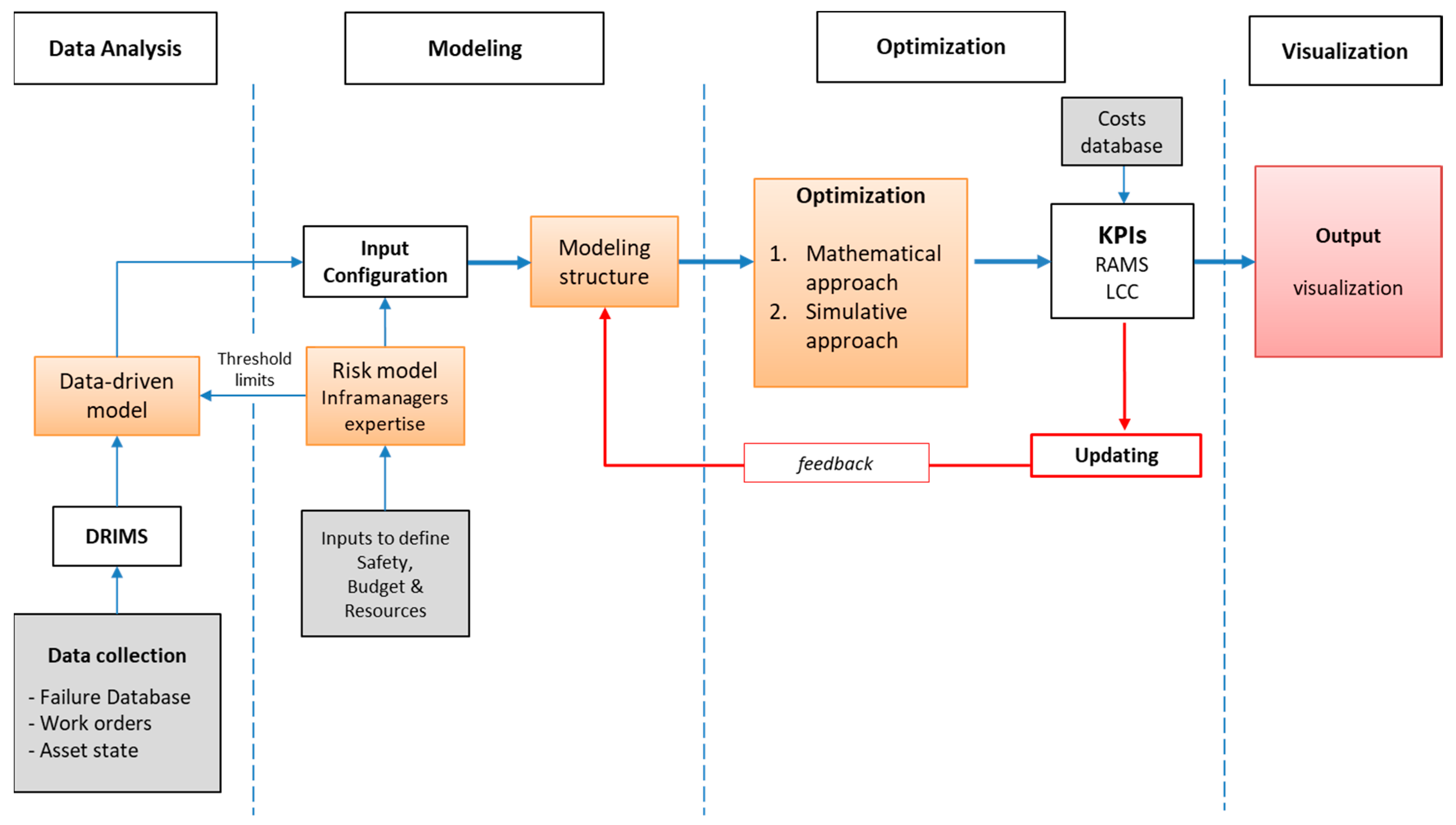
A DSS for asset management was developed according to the framework described in
Section 3.
To this aim, the monitoring system and the data acquisition system of the railway line, chosen for the case study, were upgraded by setting to acquire the track circuits’ (TCs) diagnostic data every 5 minutes (24h) and to maintain logs for future analysis.
A machine learning model for the detection of track circuits’ anomalies was developed, exploiting real-time data on track circuits’ conditions and historical data related to past failures and maintenance activities.
In particular, the used data derived from different sources and can be classified as:
Data on track circuits’ parameters (
Table 2): these data were collected from the electronic boards. The dataset contained the information used for the model development and the data structure after the cleaning and formatting operations. In particular, the shunt level was considered to build the anomaly detection model, since it was the most representative parameter of track circuit’s signal level.
FO alarms (
Table 3): these data were extracted from the central control system. An alarm is generated when a section that is expected to be free, according to the train previous position, is instead reported as occupied.
Report of maintenance interventions (
Table 4): the maintenance operators record their interventions filling a report at the end of each performed activity. This dataset was used for the validation and testing.
Detailed information regarding data collection, cleaning, and pre-formating phases is provided in [
78]. The final dataset, to be used as input for the learning algorithm, was obtained by considering a set
of
observations of the shunt level
,
, ordered by time, and the correspondent set of time instants for each track circuit. Then, the final dataset structure
was defined, consisting of
samples
for each track circuit, where each sample was built by taking for each observation
the
previous ones. The value of
was set in order to extrapolate the shunt level pattern of the previous four hours. The resulting dataset structure is shown in
Table 5.
The developed anomaly detection model was based on the machine learning technique: One-class Support Vector Machine (OCSVM).
The OCSVM algorithm, as defined in [
72,
73], is able to separate all the data points from the origin (in the feature space) and maximizes the distance from this hyperplane to the origin. The result is a binary function that returns
in a “small” region (capturing the training data points) and
elsewhere. The hyper-parameters which have been tuned are represented by the smoothing parameter
and the kernel parameter
for each track circuit.
A preliminary analysis of the OCSVM model highlighted an unstable output, identifying a high number of sparse anomalous observations (
Figure 7a).
This particular behaviour, which was mainly due to the complexity of the underlying phenomenon, presents the following issues:
Considering a visual representation for supporting maintenance operators, the output is not enough intuitive for a consistent interpretation;
Considering model performance evaluation, the output cannot be directly exploited for the computation of the performance measures.
Thus, a different solution is proposed in this work and consists of an output refinement process defined by two modules:
Anomalous Observations Count module: a new signal is generated by counting the number of anomalous observations predicted in a fixed time window (four days) preceding the prediction; output from this module is depicted in
Figure 7b;
Thresholding module: applying a threshold (dotted line in
Figure 7b) on the output of the latter module, a new binary output (anomalous/normal status) is derived (
Figure 7c). The final output is now stable and representative of an anomaly occurrence and can be easily interpreted by both an operator and an automatic system.
Since through the first module a time window which keeps in memory the number of anomalous observations that occurred in the past days was applied, the signal required some time before it dropped against to zero. Due to this behaviour, the anomaly event could last until after the maintenance action was completed, as depicted in
Figure 7b,c. Moreover, since observations corresponding to maintenance interventions were not removed from the data, the anomaly persistence, after the failure report, could be due to a maintenance action on the asset, which generates a new anomaly event.
Therefore, the proposed approach consists of the development of a final model, referred to as global model, which is built in three steps (OCSVM, Anomalous Observations Count, and thresholding module) and it is characterized by three different parameters (, , and threshold) for each involved track circuit. In other words, the global model is fitted to the track circuits selected for the study obtaining different models, which differ by the value of their parameters estimated through the analysis of the data of each specific track circuit.
More in detail, with the aim of selecting the best global model for each track circuit (i.e., tuning the global model free parameters), all the data on track circuits’ parameters of 2018 were used for the model selection, considering also the failures that occurred in the considered period. The range of the hyper-parameters tested for the OCSVM module was , was tested in a logarithmic distributed space of 60 instances ranging from to , while the thresholds were tested in a range from 1% to 99% (normalized on the maximum value of anomalous observations count found on the validation set). The model was developed using Python and the learning, validation, and testing processes were performed in the Hitachi Rail STS laboratory in a Hadoop environment, exploiting Spark Framework (the selected environment is a copy of the one operative on the field).
Regarding the system configuration modeling, it was performed at plant level, considering a Bayesian Network (BN) model [
74], using the outcomes of the anomaly detection model to set the prior probability. A BN is defined as the 2-tuple
where
is the set of the prior and conditioned probabilities and
represents a Directed Acyclic Graph (DAG) that models the network structure. The nodes are divided into parent nodes and child nodes: the parent nodes are those with outgoing arrows, while the child nodes present incoming arrows from the parent nodes.
Each node (indicated by a capital letter) is characterized by a stochastic variable that represents the probability that the node is in a
state or in another. Conditional Probabilities (CP) express the causal relationship among the nodes, evaluated as the probability,
that the node
is in
, given that
is in
,
is in
, and so on. The Prior Probabilities (PP) indicate the probabilities of being in a certain state for the nodes without parents (
root nodes) that are independent from all the other nodes.
The probability that the node
is in the state
is evaluated as follows:
where
is the joint probability that
is in
,
is in
.
Applying the Bayesian Network approach, if the failure probabilities of the components are known and the functional relationships between the different levels of the system are identified, the failure probability of the superior levels and the reliability of the overall plant can be evaluated. Moreover, the Bayesian Network can be updated every time new information on the track circuit status becomes available from the anomaly detection model, providing deep and updated knowledge on plant behaviour. In this way, the criticality of each track circuit is estimated as the consequence that its failure would have on the other system’s components.
Three phases were considered in building the Bayesian Network in
Figure 8, defined as the descriptive phase, structural phase, and relational phase.
The descriptive phase defines the system breakdown structure, that is, the system subdivision, into standardized levels: plant, system, subsystem, component, and subcomponent.
The structural phase identifies the root nodes and their prior failure probabilities (PP). Moreover, it involves the definition of the functional relationships between the elements of each level. The prior probabilities of the root nodes are derived by the data analytics results.
The relational phase evaluates the Conditional Probabilities for each child node and the posterior conditional failure probabilities (PCP) for each level. Then, the reliability of the plant is computed, given the prior failure probability of the root nodes and the conditional probability of each child node. In this way, the criticality of the track circuit in terms of impact on the overall system is determined.
Finally, the optimization was performed considering a risk-based scheduling model that allowed planning of the maintenance activities via a Mixed Integer Linear Programming (MILP) problem [
75]. In the MILP problem the failure probability and the criticality of each track circuit, evaluated through the Bayesian Network, were then used to prioritize the interventions. As mentioned, the signaling system is a fail-safe system, since the safety of trains operation is always guaranteed even if a track circuit’s failure occurs, because the track section is automatically reported as occupied. Nevertheless, the false occupancy is a critical failure for rail operations since it has relevant consequences for trains’ circulation, usually implying the interruption of the service. Therefore, the optimization model took into account the risk of service disruptions, which was estimated by considering the criticality of the track circuit and its condition. The criticality was evaluated by applying the Bayesian Network approach, as the impact that a failure would have on the operation of the rail line. The status of track circuit was instead provided by the data-driven model.
In order to consider the risk in the decision-making process, the risk of a track circuit failure was considered in the objective function as a weight
, as described in Equation (5):
where:
is the importance of the term of the objective function, defined by the decision-maker;
is the risk of failure of track circuit ;
is the time needed to conclude the maintenance activity on the track circuit executed by the maintenance crew ;
is the difference between the planned time of execution and the expected one according to the criticality order;
is the total path length covered by the maintenance crew ;
is the difference of the path lengths covered by the maintenance crews and ;
is the difference of the number of maintenance activities allocated to maintenance crews and .
The optimization model made it possible to schedule the maintenance interventions in a sustainable way, taking into account different aspects related to sustainability. In particular, the optimization model considered track circuits’ status and criticality, preventing false track occupancies events and thus minimizing the risk of service disruptions. This implies a reduction of corrective maintenance activities that represent high costs for the infrastructure manager and for the society. Moreover, the model evaluated the optimal use of resources (maintenance crews), balancing the workload of each crew and guaranteeing the minimization of the covered distance to reach the assets to be maintained. To do this, the position of each track circuit along the line was considered, as well as the time needed for the crews’ movements.
Finally, the available time for maintenance was taken into account, evaluating the best allocation of maintenance activities to the available time windows; that is, those intervals during which the train circulation was stopped.
The optimization problem considered real operational constraints of the rail environment, such as the time and resources limitation. These limitations became mathematical constraints, expressed according to the formulation provided by Consilvio et al. [
75].
Therefore, the efficiency and the sustainability of the maintenance process were pursued, avoiding unnecessary interventions and preventing failures. The benefit is the limitation of corrective maintenance activities and the reduction of the needed time for maintenance execution.
It is worth mentioning another important feature of the Decision Support System, that is, its capability of dealing with the uncertainty. Since real-world operational scenarios are characterized by a high level of uncertainty and unexpected events may occur at any time, the planning model is able to adapt its results in a dynamic way, in different situations. In particular, the optimization model updated the maintenance plan, when updated inputs and information regarding the track circuits’ status are provided by the data-driven model, or when an alarm is detected.
Moreover, since the anomaly detection is characterized by a given uncertainty, which is evaluated and reported in the Results section, the Decision Support System took into account this uncertainty, by considering the sensitivity of the solution to this variability.
Other adaptations of the previously defined maintenance plan were computed in case of delays of maintenance execution or unexpected unavailability of resources.
Regarding the output visualization, an HMI was developed to support the operators.
In
Figure 9, the dashboard is represented with the information regarding the variation over time of the track circuits’ parameters and the anomaly detection. Moreover, a schematic view of the line is provided to the user that can select the station and the track circuit to be visualized.

 ,
, 


