On Applying Machine Learning and Simulative Approaches to Railway Asset Management: The Earthworks and Track Circuits Case Studies

Abstract

The objective of this study is to show the applicability of machine learning and simulative approaches to the development of decision support systems for railway asset management. These techniques are applied within the generic framework developed and tested within the In2Smart project. The framework is composed by different building blocks, in order to show the complete process from data collection and knowledge extraction to the real-world decisions. The application of the framework to two different real-world case studies is described: the first case study deals with strategic earthworks asset management, while the second case study considers the tactical and operational planning of track circuits’ maintenance. Although different methodologies are applied and different planning levels are considered, both the case studies follow the same general framework, demonstrating the generality of the approach. The potentiality of combining machine learning techniques with simulative approaches to replicate real processes is shown, evaluating the key performance indicators employed within the considered asset management process. Finally, the results of the validation are reported as well as the developed human–machine interfaces for output visualization.

1. Introduction

The digital transformation of rail systems makes it possible to increase the sustainability of asset management (AM) thanks to the introduction of decision support tools able to use the data from the field in order to optimize the use of resources, reducing assets’ life cycle costs (LCC). These decision support tools receive inputs from railway digital monitoring systems, able to provide a considerable amount of data in real-time that can be then elaborated and analyzed. Artificial intelligence techniques, and, in particular, machine learning methods, can be applied in order to extract information from the available data, guiding decision-making, reducing human effort, and achieving a high level of automation in railway asset management process.

The objective of this study is to show the applicability of machine learning and simulative techniques within the generic framework of a Decision Support System (DSS) for rail asset management decision-making, developed within the H2020 Shift2Rail Project In2Smart (Intelligent Innovative Smart Maintenance of Assets by Integrated Technologies). The framework has been tested in-lab and validated within In2Smart reaching the Technology Readiness Level (TRL) 4. Currently, the framework is under in-field implementation within the follow-up project of In2Smart, In2Smart2, to reach TRL 6/7. In particular, the general intelligent asset management framework, proposed by In2Smart [1,2], is composed by: (i) the Railway Information Measuring and Monitoring System (RIMMS); (ii) the Dynamic Railway Information Management System (DRIMS), and (iii) the Intelligent Asset Management Strategies (IAMS).

The presented paper describes the application of innovative techniques within the general framework to two case studies: the first one is related to the asset management of earthworks at strategic level, while the second one deals with the maintenance of track circuits at tactical and operational level. The main building blocks of the Decision Support System and their interactions are described, showing how the use of predictive analytical techniques and simulation models could foster the optimization of asset management and the prolongation of asset lifetime. The approaches and methodologies used for the development of the different building blocks of the asset management framework are different in the two case studies, but they both follow the general framework, highlighting the applicability of the proposed asset management approach to different contexts.

Furthermore, the key performance indicators (KPIs) for the decision makers are identified and the results of the validation are provided. Finally, the developed human–machine interface (HMI) for the output visualization is described, showing the usefulness of the system in real-world scenarios.

2. Literature Review

Rail transport is rapidly becoming digitalized, with an increasing role of digital technology in all aspects of the rail sector. The digital revolution is opening up many opportunities for railway operators and infrastructure manager. The digital transformation of rail systems makes it possible to increase the sustainability of asset management thanks to the introduction of decision support tools, able to exploit data from the field in order to optimize the use of resources, reducing assets’ life cycle costs (LCC). The importance of pursuing sustainability goals in railway asset management is highlighted by many works in the literature [3,4,5,6,7].

In particular, the applied maintenance strategy may have a significant impact on life cycle cost, since poor maintenance processes imply downtimes and consequent costs.

In many sectors, a preventive approach to maintenance has become key for achieving the sustainability targets, such as in Industry 4.0 [8], in the asset management of civil infrastructure [9] and linear assets [10], such as roads and bridges [11].

In the rail sector, works deal with the introduction of sustainability concepts in asset management, applying a whole-system life cost analysis [12,13,14].

To do this, multi-criteria decision analysis frameworks that incorporate sustainability criteria over the whole life cycle have been developed in the literature [15], considering different rail assets, such as rail signaling and control systems [16].

The possibility of receiving data in real-time, from automatic and fully integrated monitoring systems, makes it possible to develop a more sustainable and digitally supported asset management [17,18]. Moreover, a context-aware decision-making can be achieved, providing infrastructure operators, system suppliers, and construction companies with comprehensive information. Finally, with the introduction of Internet of Things (IoT) sensors, some assets are becoming able to perform self-diagnostics and even self-repairing [19,20].

In an eMaintenance context, IoT devices and smart sensors perform condition monitoring, collecting data to be used by machine learning algorithms, to achieve predictive maintenance strategies [21]. Therefore, asset management and, in particular, maintenance can be improved through the use of networked technologies for condition monitoring and asset information system. In particular, new prognostic approaches could make it possible for operators to be well aware of asset management and maintenance needs before failure.

Different techniques of data analysis are already applied in the rail sector, such as Artificial Neural Networks (ANN), Support Vector Machines (SVM), and Random Forests (RF) [22,23,24,25]. Regarding asset management, different studies exist in the literature [26,27,28]. Ghofrani et al. [29], Thaduri et al. [30], Pipe et al. [31], and Lee et al. [32] developed data-driven models able to forecast the status of assets in order to achieve predictive maintenance strategies.

Some studies have been developed to integrate data-driven models within a decision-making framework for railway maintenance, considering different assets and case studies. Morant et al. [33] and Yang et al. [34] considered, for example, the issue of maintaining the signaling systems of a rail line, while Núñez et al. [35], Jamshidi et al. [36], and Consilvio et al. [37] focused their studies on the maintenance of rail tracks.

In these works, the availability of data made it possible to achieve a more efficient and sustainable maintenance strategy.

Moreover, with the digital revolution, the concept of a “digital twin” is becoming a powerful and valuable instrument to make high-quality decisions, resulting from the transformation of data into actionable insight to improve decision-making.

The digital twin is a dynamic digital representation of an asset, system, or process [38]. This virtual representation is more than just a model of the physical object, since it can receive continuous, real-time data from the asset. The sensors measure assets’ parameters and the data are sent in real-time and visualized by the digital twin. Therefore, the virtual replica is updated according to the received information, providing a real-time representation of the real system. Digital twins are key to improve situational awareness and to proactively anticipate maintenance faults, allowing testing of future scenarios, thus enhancing asset performance [39]. Therefore, thanks to the updated knowledge of asset status, the Decision Support System is then able to turn the information into decisions in an automated way [40]. The DSS becomes the platform where digital twin, based on data analytics, simulative and modeling approaches, and artificial intelligence makes it possible to access real-time data and translate it into data-led decisions. Three-dimensional representations of physical assets are built by using Building Information Modeling (BIM) [41,42], while digital twins of complex systems and processes are built by other instruments, such as agent-based models, discrete event simulations, Petri nets (PN), and Bayesian Networks (BN) [43,44]. Studies emphasize the strong link between the application of digital twin technologies and the achievement of high sustainability levels in asset management [45]. In particular, for the rail sector, some evidence has been provided by Kaewunruen et al. [46] and Neves et al. [47] considering rail turnouts systems and rail tracks, respectively.

Therefore, the basic idea of the present paper is to combine data analytics, simulative and modeling approaches, and machine learning techniques in order to build a system for railway asset management decision-making. Examples of simulative approaches are already available in the literature. Baglietto et al. [48], Colla et al. [49], and Di Febbraro et al. [50] applied simulative techniques to assess the reliability, availability, and vulnerability of rail networks, comparing what-if scenarios.

In particular, the Petri net methodology was considered in order to model asset degradation in the rail sector by Rama et al. [51] for rail superstructure, by Andrews et al. [52] and Shang et al. [53] for track degradation, and by Le et al. [54] for rail bridges.

Bayesian network approaches are mostly applied in the rail sector for the reliability evaluation of technological components and signaling system elements, such as by Liang et al. [55] for level crossings, Jiang et al. [56] for track circuits, and Baigen et al. [57] for train ground communication subsystems.

Nevertheless, these methodologies can now be applied within a new simulation modeling paradigm, by combining the advantages of machine learning and data-driven models with the strength of simulative approaches [58,59]. This allows an improvement of context awareness, real-time knowledge and dynamic aspects of simulation, enhancing the deductive potentiality of the simulative approach in reproducing what-if scenarios.

Regarding the decision support algorithms, studies available in the literature [60,61,62] applied mathematical programming to optimize the use of resources and to plan maintenance activities. The considered issues were modeled as multi-objective optimization problems, considering different key performance indicators, relevant for the infrastructure manager, and operational constraints, such as trains’ operation.

An important aspect to be considered by the decision support system is the uncertainty of the degradation process in maintenance planning. The stochastic aspect of predictive maintenance is discussed in Andrews et al. [63], Baldi et al. [64], and Consilvio et al. [65] through simulative, rolling horizon, and stochastic programming approaches, respectively.

Nevertheless, the development of Decision Support Systems able to integrate data-driven algorithms and modeling methodologies has not received the deserved attention yet.

This paper tries to move some steps towards the development of a digital twin for the rail asset management process by merging data analysis, machine learning, and simulation techniques to build a Decision Support System able to analyze real-time data and translate them into automated decisions. The aim is to improve the sustainability of the asset management process, considering different time horizons: the first case study considers the asset management at strategical levels, evaluating the more sustainable mix of interventions (maintenance activities, refurbishments, and renewals), considering a whole life cycle cost approach, the second case study instead deals with a short time horizon and it is aimed at improving maintenance operations, reducing the costs due to unexpected failure and service disruptions, in order to achieve a more sustainable maintenance strategy.

3. Building the DSS

A general framework for decision support systems in maintenance and interventions planning has been defined within the In2Smart project [66], in accordance with the ISO 55000 standard [67] and the UIC guidelines for asset management [68].

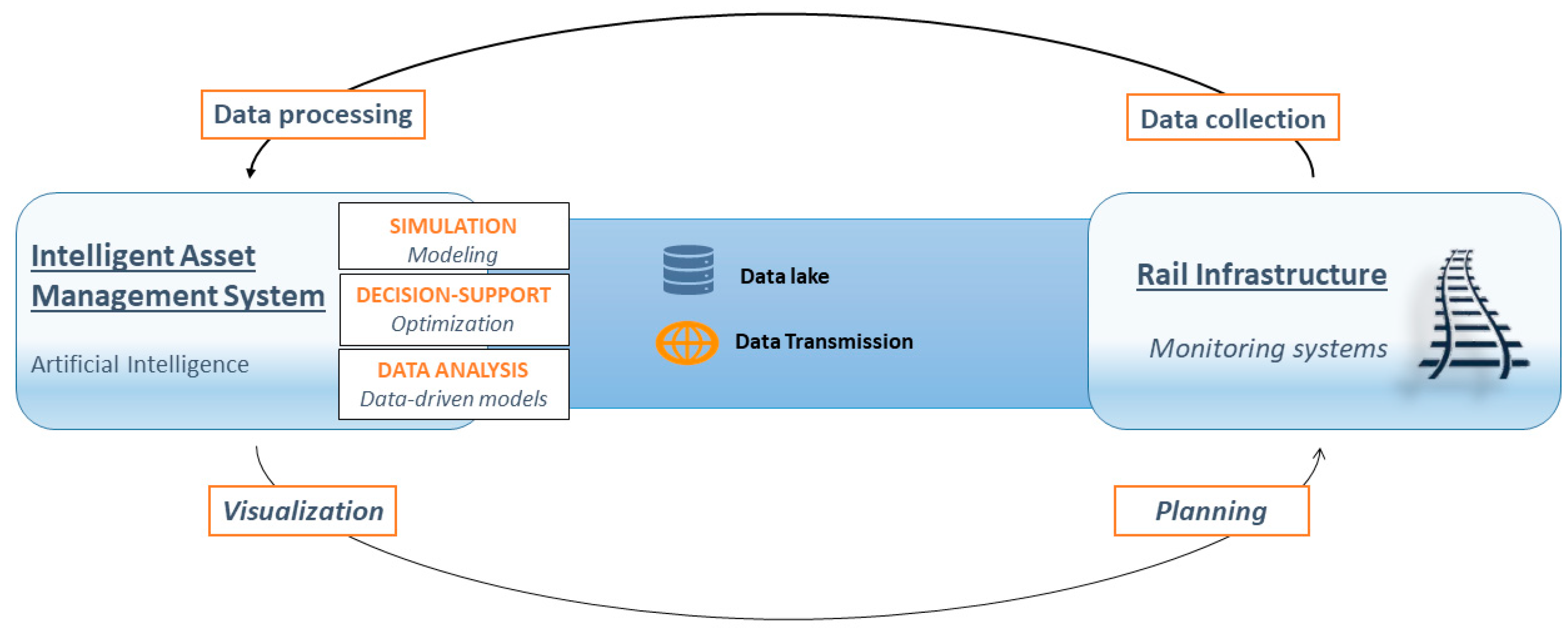
In this paper, according to the general In2Smart framework, four main general stages were identified to build the DSS, as depicted in Figure 1:

• Data analysis: the available data are exploited to evaluate the asset condition;
• Modeling structure: the system configuration is modeled in order to have a virtual representation of complex systems and to identify the relationships between components and their interactions;
• Decision-making: a set of solutions are identified for the decision makers on the basis of some identified KPIs. Two main approaches are commonly used: simulative and computational. One of the main aspects of the optimization model is the uncertainty management (consisting usually in feedbacks) to deal with the stochastic nature of degradation process. The relevant KPIs for the decision-makers are computed, as well as the performance of the DSS and the goodness of the provided solutions. The goal is to achieve a sustainable asset management strategy, in terms of sustainable use of resources, with a consequent reduction of the life cycle cost, and the minimization of corrective maintenance activities, which have high costs for the society;
• Output visualization: an HMI is developed for the visualization of the DSS results.

According to the general framework, the core elements and interactions of the developed decision support system are represented in Figure 2.

In the following sections, the application of innovative approaches based on machine learning and simulation techniques within the proposed framework is described, showing the applicability of the framework to two different case studies. In particular, the first one dealt with the strategic planning of rail earthworks asset management, while the second one was related to tactical/operational planning of track circuits’ maintenance operations.

Different methods were applied to develop each building block of the framework in the two case studies, according to the considered asset and time horizon. In particular, three main building blocks were developed: the analytics/data-driven model, the modeling structure for the simulation, and the decision support/optimization module.

In particular, in the earthworks case study the data-driven model was based on the K-means machine learning approach [69], the modeling was made by a Petri nets approach [70], and the decision support was based on Monte Carlo simulations [71] for scenario comparison.

In the track circuits’ case study, a One-Class Support Vector Machine [72,73] was applied to build the data-driven model, the Bayesian Network approach [74] was used for the modeling and simulation, and a mixed integer linear programming mathematical model [75] was developed for the optimization.

In the following sections, the two case studies are described, detailing the applied methods.

4. Case Study A: An Intelligent Asset Management System for Rail Earthworks

The objective of this case study was to enhance the sustainability of the rail earthworks (EWs) asset management process by applying carefully selected data analytics techniques and simulative models, using the extracted information to build an intelligent asset management system at strategic level. In particular, the asset management model developed in the case study was based on machine learning clustering methods and Petri net models. The DSS enables the computation of the optimal work volumes at the portfolio level, which are able to sustain high asset performance at the lowest life cycle cost.

The considered assets consisted of 191,000 earthworks of the UK railway infrastructure, managed by Network Rail. The collected data were related to earthworks condition, EWs failure, and track geometry evolution for the selected railway lines, as reported in

Table 1. Data type and content.

Data Sources	Content
Earthworks assets register	Earthworks assets characteristics, location, and examination date, including: (a) Earthwork type (embankments, soil, and rock cuttings) (b) Slope angle height category (c) Soil composition (d) Earthwork condition (EHC) (e) Mileage/UP or DOWN (f) Survey date (g) Hazard index (EHI)
Weather records	Weather records, including: (a) Measurement date and time (b) Weather cell (c) Rainfall across 3-hour interval (d) Soil Moisture Index (SMI) every 12 hours
Track geometry measures	Track geometry parameter values, localization, and examination date, including: (a) Top deviations Standard Deviation (SD) (35 and 70 λ) (b) Alignment Standard Deviation (35 and 70 λ) (c) Other Track Geometry parameters (twist, gauge)
Earthworks failures	Earthworks failures register, including the failure type and description

.

An unsupervised anomaly detection classification method, specifically a partitioning clustering method [69], was applied: the K-means algorithm.

This algorithm requires the user to define the number of clusters, $k$, which will be used to define $k$ centroids, one for each cluster. The objective function $J$ is given by:

$$Minimize J={{\displaystyle \sum }}_{j=1}^k{{\displaystyle \sum }}_{i=1}^n{\Vert x_i^{\left(j\right)}-c_j\Vert }^2,$$

(1)

where ${\Vert x_i^{\left(j\right)}-c_j\Vert }^2$ is a chosen distance measure between a data point $x_i^{\left(j\right)}$ and the cluster centre $c_j$. The procedure consists of initially randomly choosing k centroids and assigning each data point to the nearest centroid. Once each data point has been assigned to a centroid and thus to a cluster, the positions of the k centroids are recalculated. The process ends when the centroids no longer move. Anomalies will be defined as a set of objects that are considerably dissimilar to the rest of the data, that is, data points that do not strongly belong to any cluster.

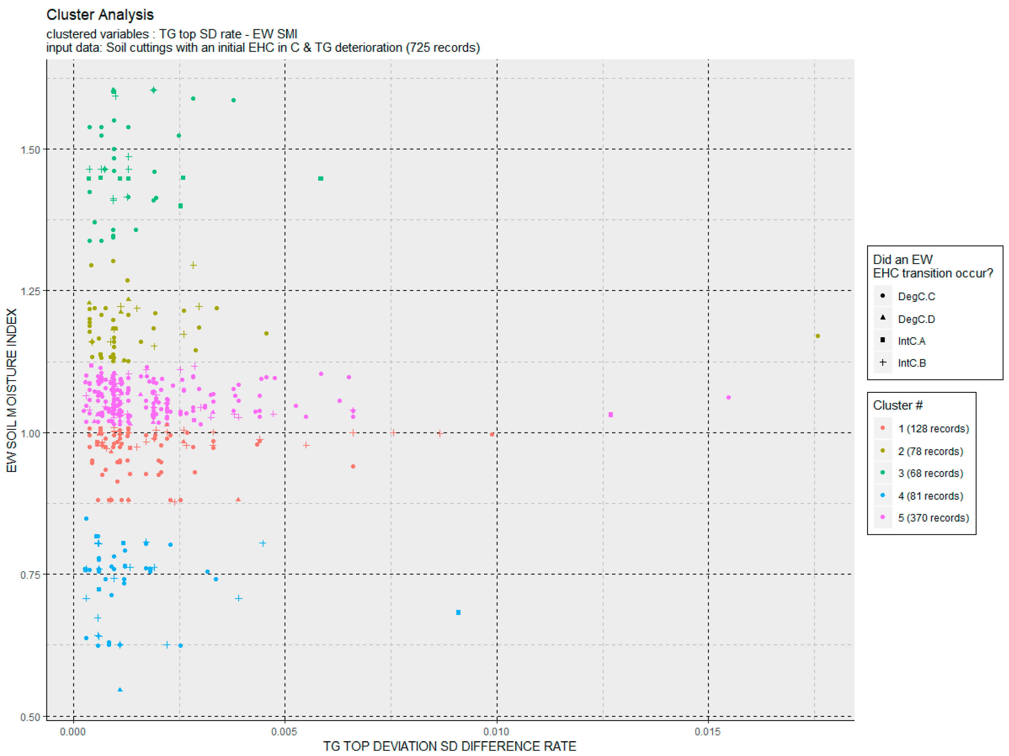
In Figure 3, the results of the data analysis are reported.

This data-driven analysis, along with other analyses that provided preliminary information, as explained in deliverables 8.1 and 8.2 of In2Smart [76,77], was the baseline for the computation of the parameters that were required by the PN model to set up the simulations of the degradation process. A Petri net [70] is a 3-tuple $PN=\left(S, T, W\right) \left\{\backslash displaystyle \left(S,T,W\right)\right\}$, where:

• $S$ is a finite set of places;

• $T$ is a finite set of transitions;

• $S$ and T are disjointed, i.e., no object can be both a place and a transition;

• {\displaystyle W:(S\times T)\cup (T\times S)\to \mathbb {N} } $W$ is a multiset of links with non-negative integer link weights; note that two places or two transitions cannot be connected by any link.

The parameters, provided by the data analysis, consisted of the probabilities of transition of an asset (token) from one condition state to another and the time distributions related to a certain condition state transition.

The developed PN modeling structure was based on the subdivision of the earthworks portfolio in cohorts or groups of similar EW assets. The modeling structure was able to consider the following factors:

• The different earthworks subsystems:
  • three types of earthworks, i.e., embankments, soil cuttings, and rock cuttings, modeled in successive simulations;
  • five earthworks conditions (EHC) from A to E plus failure (F), which were represented as places in the PN;
  • five Earthwork Asset Criticality Bands (EACB from 1 to 5), which were again modeled in successive cohort simulations; and
  • additional parameters or characteristics such as rainfall or soil composition that could constitute additional bases to define further granular EW cohorts.
• The type of interventions to be applied, i.e., maintenance, refurbishment, or renewal, which was represented in the model through different PN places;
• The intervention mixes, which were defined as the percentages of assets to be intervened. As stated above, the options were to maintain, refurbish, renew, or not to act at all;
• Deliverability and availability of resources. The model must be able to take into account the capacity of the infrastructure manager to intervene (i.e., the deliverability) over a control period (CP) of five years.

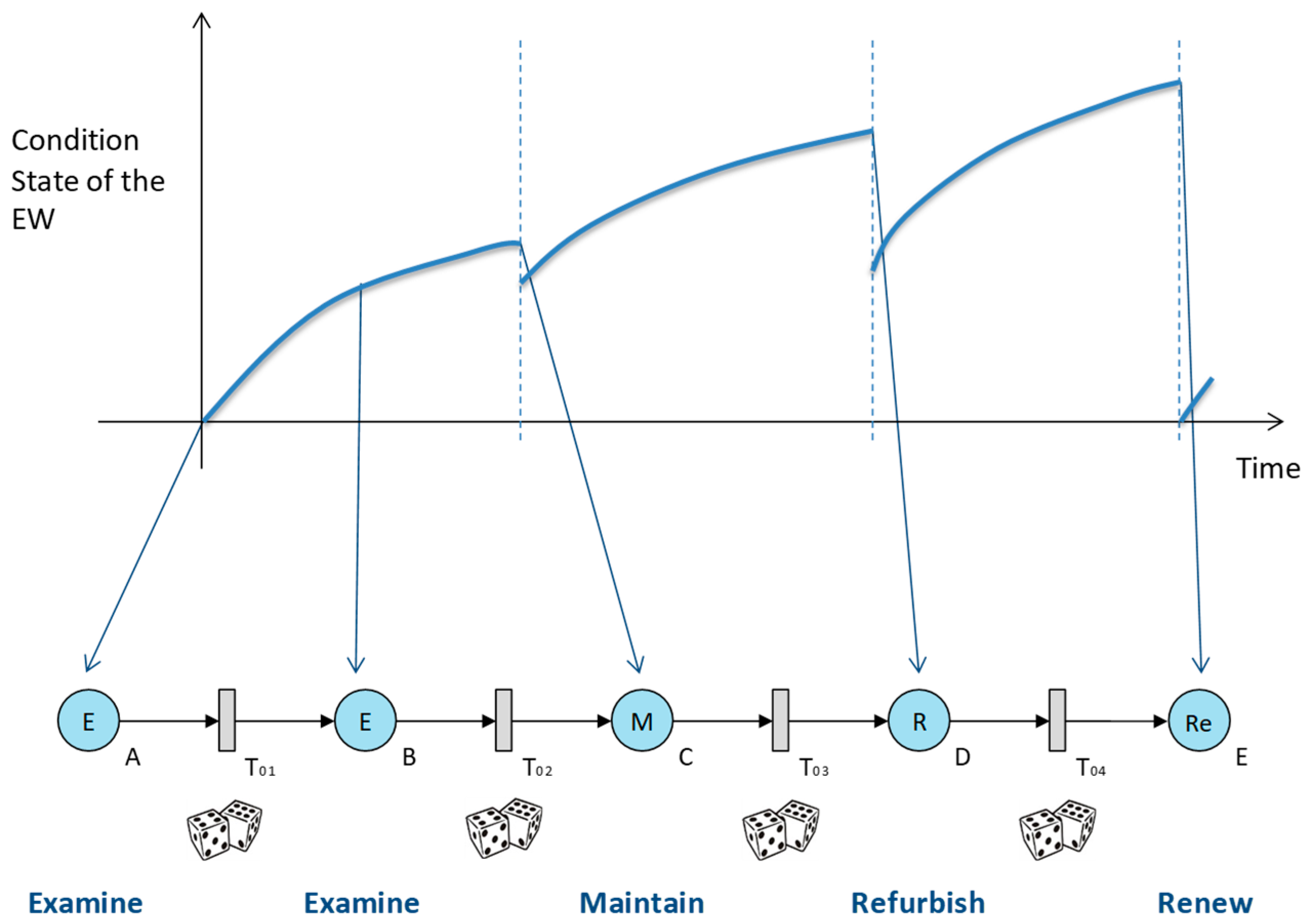
A graphical and simplified representation of the PN model, developed in this case study, is shown in Figure 4. Condition states A to E are represented by places, and the generic transitions 1 to 4 represent the degradation processes and the possible interventions to be applied.

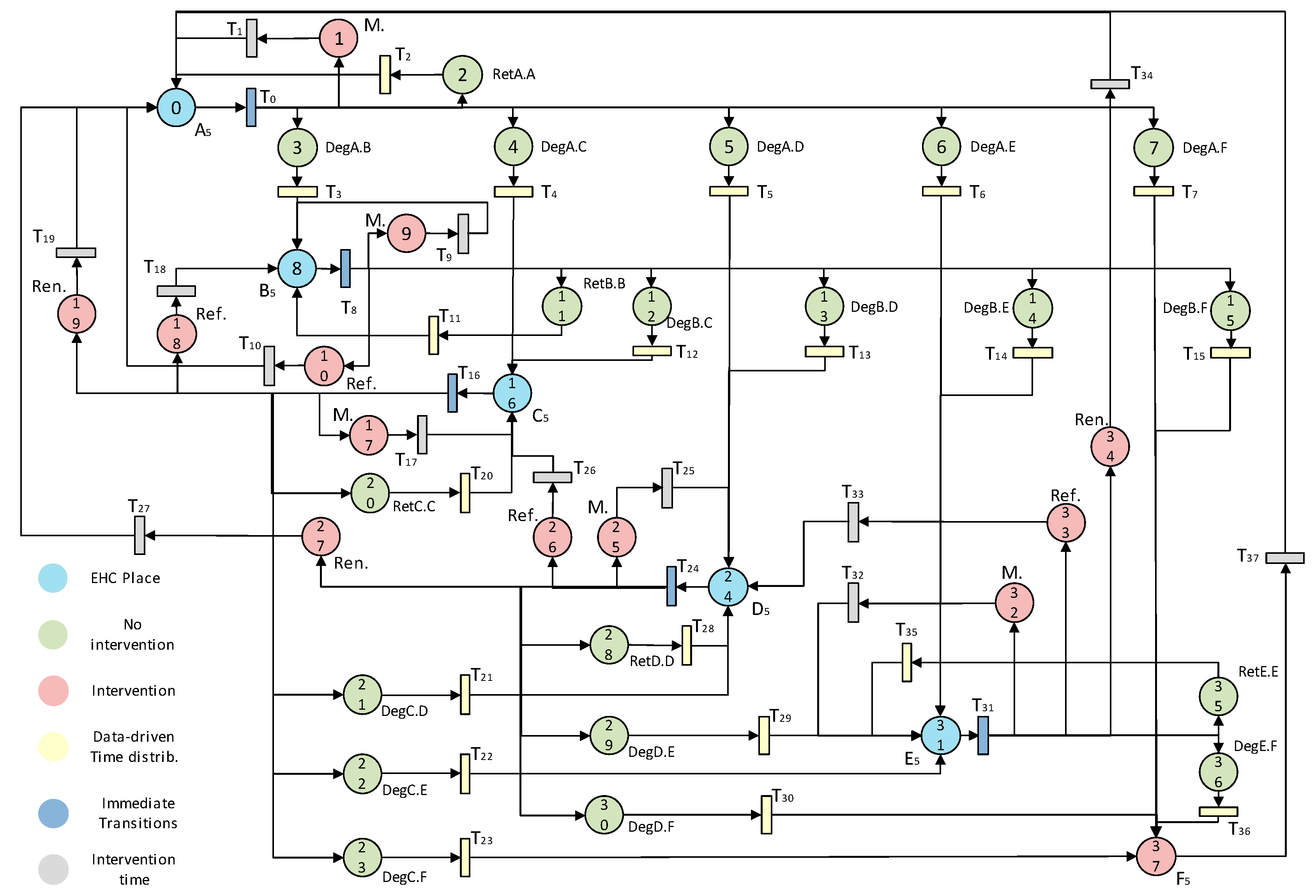
The complete simulation model for the soil cutting cohort is depicted in Figure 5.

The Petri net model made it possible to take into account the uncertainty of the asset status estimation, considering a probability distribution for each transition, correspondent to a variation of the asset status (i.e., changes in EHC). Moreover, since a long-term time horizon, characterized by high uncertainty, was considered, different scenarios were compared, evaluating the solution that was able to give stable results in a high number of scenarios.

Therefore, the robustness of the solution to the uncertainty of long-term scenarios was guaranteed.

The optimization performed in this case study was an iterative simulation-based process using the PN modeling structure. A significant number of runs of Monte-Carlo simulations [71] were executed in order to compute a converged set of results for each particular intervention scenario. The outputs from the simulations, applying different intervention mixes, provided information regarding the aggregated degradation patterns and the number of interventions computed in each scenario. All this information could then be used to compute whole life costs and finally perform the optimization via a comparison of scenarios. The outcome of the scenarios for each cohort must also comply with the resources and budget constraints from the infrastructure manager. Therefore, three KPIs were defined for the optimization process.

• Intervention volumes: This was the number of earthworks to be renewed, refurbished, or maintained at a certain CP of the simulation. Five intervention deliverability bands defined by the Infrastructure Manager, which stated the percentage of assets that could be intervened, were considered. These five bands were the following (in ascending order of intervention volume): not sensible, deliverable, probably deliverable, possibly deliverable, and not deliverable;
• Intervention costs: These can be calculated using Equation (2):

  $$LCC={\displaystyle \sum }_{i=1}^N\left(n_m^i·c_m^i+n_r^i·c_r^i+n_{ren}^i·c_{ren}^i\right)$$

  (2)
  The computed overall costs depend on the total number $N$ of assets in a cohort, hence:
  • $n_m^i,$$n_r^i$ and $n_{ren}^i$ represent the number of maintenance, refurbishment, and renewal interventions on an asset $i$;
  • $c_m^i,$$c_r^i$ and $c_{ren}^i$ represent the unit intervention costs for the type of intervention;
• Risk and Condition (R&C) scores: These are two factors defined on the basis of the earthworks conditions (EHC) and the Earthwork Asset Criticality Bands (EACB). They were used to track the state of the infrastructure along the simulations.

Following the definition of these KPIs, it is important to highlight that the evaluation of the life cycle cost is closely linked to the sustainability of both the asset management decisions and the state of the infrastructure itself. This evaluation was conceived (following the requirements of the Infrastructure Manager) as an iterative process where the range of analyzed scenarios was, first of all, evaluated according to their risk and only then according to the intervention costs. This puts the sustainability and safety of the infrastructure in the first place.

This iterative two-stage vision of the management of the assets led to the optimization process, explained in more detail in the next paragraph, which, effectively, ensures that the state of the infrastructure over time fulfils the required level of safety and sustainability, taking into account the Risk and Condition scores. The Infrastructure Manager can, therefore, assess which asset management scheme of intervention can provide a sustainable infrastructure over time, avoiding unsustainable short-term policies. It is important to note that the costs cannot be specifically reported in this paper since they constitute sensitive information for the Infrastructure Manager.

In detail, the optimization process generally followed four basic steps: (i) the simulations were performed varying the intervention mixes; (ii) the simulations with intervention volumes at the “not sensible” or “not deliverable” bands were discarded; (iii) a certain band of R&C scores was selected, where additional case scenarios were disregarded; and (iv) the intervention costs were optimized, considering all the possibilities left from step iii.

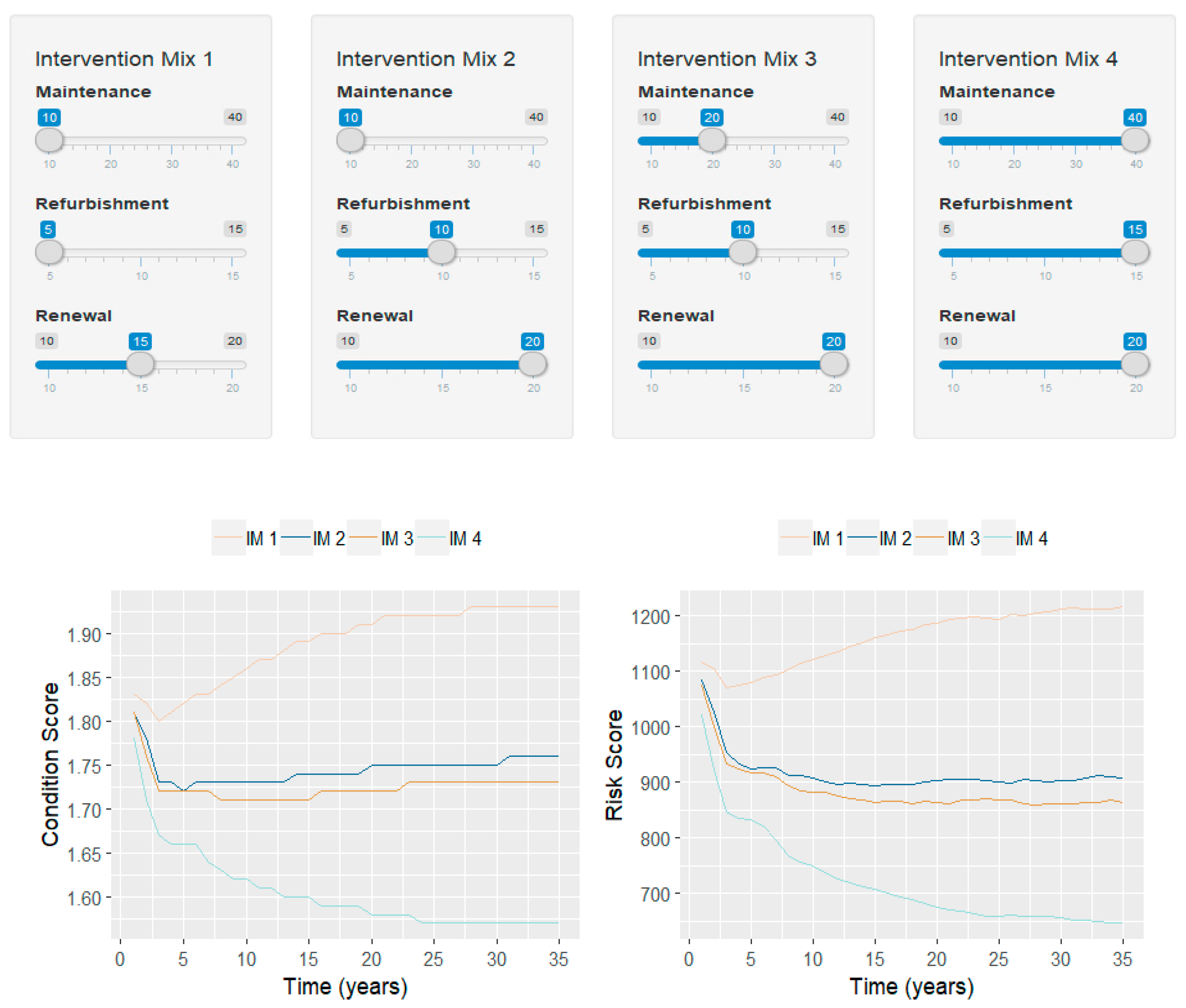
In order to make the outcomes of this prototype available for the final user, including the data analytics and IAMS findings, a human–machine interface (HMI) was developed using RStudio’s Shiny App platform. Figure 6 shows an example presenting four intervention mixes that can be modified by the user.

Once the intervention mixes were selected in the upper panel of Figure 6, a set of results was provided according to the four chosen intervention schemes. These results included the following KPIs over the simulation time horizon (in this case, 35 years):

• The number of annual interventions of each type (maintenance, refurbishment, and renewal);
• The annual intervention costs;
• The aggregated costs and predicted failures over the whole simulation;
• The evolution of the Risk and Condition Scores, as depicted in Figure 6.

These KPIs were numerical measures defined by Network Rail to compute the state of the infrastructure at a given point in time.

The Risk and Condition Scores should be treated as relative measures. As mentioned, the earthwork condition (EHC) can be defined as the statistical likelihood that a particular asset may fail. The EHC divided the assets into five categories from A to E, where category A represents assets with the lowest probability to fail and category E represents the assets with the highest failure probability. There is also a further state which represents the failure (state F).

Moreover, earthwork criticality is a quantified measure of the safety consequences that would arise if the failure of a specific earthwork occurs. This criticality is defined as the Earthwork Asset Criticality Band (EACB) and it is divided in five bands, from 1 to 5. Band 1 has the lowest consequences and band 5 has the most severe consequences. The safety risk is computed as the product of the likelihood that the earthwork will fail (EHC) and the safety consequence if it fails (EACB). The evaluated risk is then compared to some confidential safety thresholds established by the Infrastructure Manager in order to define the acceptability of a given scenario of interventions. In a particular simulation, a decrease in the Risk and Condition Scores reports that the overall state of the portfolio of earthworks is improving and, therefore, there is a lower risk of failure. Likewise, an increase in these parameters means the infrastructure is degrading and, hence, there is a higher risk of failure.

The results in Figure 6 show how intervention mix 1 increased the R&C scores and hence the state of the infrastructure degrades due to the low percentage of selected interventions. Intervention mixes 2 and 3 maintained the health of the infrastructure relatively constantly. Finally, intervention mix 4 improved the overall state of the infrastructure over time, as the selected intervention mix imposed much higher probabilities of intervention, which is reflected in the final results. Therefore, the developed system allows the management of the portfolio of earthworks by selecting the intervention scenarios that provide a sustainable and safe level of risk.

5. Case Study B: Track Circuits—False Track Occupancies Mitigation

The case study was aimed at the development of a tactical/operational asset management strategy to optimize the maintenance activities related to a rail line in Italy, focusing on a particular kind of asset: the track circuit.

The final goal was the mitigation of false track occupancy events (FO). A false occupancy event occurs when a track section is erroneously reported as occupied, even if no train is present on it. The signaling system is fail-safe, since the safety of train operation is always guaranteed, even if a track circuit’s failure occurs. Nevertheless, false occupancy is considered a failure characterized by a high criticality for the operation of a railway line, due to its impact on the rail service.

The track circuit is characterized by a signal whose level should stay within a given range of nominal values. When an occupancy event occurs and a train enters the line section, the signal level decreases due to a short-circuit caused by the presence of the train wheels and the related axle. Therefore, the signal is no more able to reach the receiver, a nil value of the signal is registered, and the track is considered occupied. If a decrease in the signal level occurs even if the line section is free, a false occupancy is detected.

A DSS for asset management was developed according to the framework described in Section 3.

To this aim, the monitoring system and the data acquisition system of the railway line, chosen for the case study, were upgraded by setting to acquire the track circuits’ (TCs) diagnostic data every 5 minutes (24h) and to maintain logs for future analysis.

A machine learning model for the detection of track circuits’ anomalies was developed, exploiting real-time data on track circuits’ conditions and historical data related to past failures and maintenance activities.

In particular, the used data derived from different sources and can be classified as:

• Data on track circuits’ parameters (

  Table 2. Data on track circuits’ parameters.

  Variable	Definition
  Timestamp	Time instant and date of the recorded parameter’s value
  Station	Position of the track circuits’ board rack
  Track circuit ID	Identification number of track circuit
  Primary/Backup	Type of track circuit’s board
  Shunt Level	Parameters of track circuit’s signal
  Variance	Parameters of track circuit’s signal
  Raw Signal Level	Parameters of track circuit’s signal
  Receive Level	Parameters of track circuit’s signal
  Direction	Direction of track circuit
  Active	Board that is working at a given time instant
  Occupied	Binary value equal to 1 if the track is occupied by a train, 0 otherwise

  ): these data were collected from the electronic boards. The dataset contained the information used for the model development and the data structure after the cleaning and formatting operations. In particular, the shunt level was considered to build the anomaly detection model, since it was the most representative parameter of track circuit’s signal level.
• FO alarms (

  Table 3. False Occupancy alarms.

  Variable	Definition
  FMT	Information provided by the alarm
  TS	Time instant and date of the alarm
  CP	Station in which the alarm occurred
  CX	Track position related to the alarm
  STY	Type of the log file (event or alarm)
  TC ID	Track circuit’s identification code
  EQ	Identification code of the alarm

  ): these data were extracted from the central control system. An alarm is generated when a section that is expected to be free, according to the train previous position, is instead reported as occupied.
• Report of maintenance interventions (

  Table 4. Report of maintenance interventions.

  Variable	Description
  ID	Identification code of the maintenance activity
  Opening Date	Date on which the maintenance order was opened
  Opening Time	Time at which the maintenance order was opened
  Closing Date	Date at which the maintenance order was closed
  Closing Time	Time at which the maintenance order was closed
  TC ID	Identification code of the involved track circuit
  Failure Cause	Cause of the failure
  Maintenance action	Type of the performed maintenance activity

  ): the maintenance operators record their interventions filling a report at the end of each performed activity. This dataset was used for the validation and testing.

Detailed information regarding data collection, cleaning, and pre-formating phases is provided in [78]. The final dataset, to be used as input for the learning algorithm, was obtained by considering a set $S$ of $n$ observations of the shunt level $s_i$, $i=0,\dots ,n$, ordered by time, and the correspondent set of time instants for each track circuit. Then, the final dataset structure $X=\left[x_0,x_1,\dots ,x_{n-m}\right]$ was defined, consisting of $n-m$ samples $x_j$ for each track circuit, where each sample was built by taking for each observation $s_i$ the $m$ previous ones. The value of $m$ was set in order to extrapolate the shunt level pattern of the previous four hours. The resulting dataset structure is shown in

Table 5. Final dataset structure for a single track circuit.

Features	Description
$TS$	Timestamp equivalent to the observation index $t$
$s_{\mathrm{t}}$	Shunt value observed at $t$ ($t=TS$)
$s_{\mathrm{t}-1}$	Shunt value observed at $t-1$
…	…….
$s_{t-m}$	Shunt value observed at $t-m$

.

The developed anomaly detection model was based on the machine learning technique: One-class Support Vector Machine (OCSVM).

The OCSVM algorithm, as defined in [72,73], is able to separate all the data points from the origin (in the feature space) and maximizes the distance from this hyperplane to the origin. The result is a binary function that returns $+1$ in a “small” region (capturing the training data points) and $-1$ elsewhere. The hyper-parameters which have been tuned are represented by the smoothing parameter $\nu$ and the kernel parameter $\gamma$ for each track circuit.

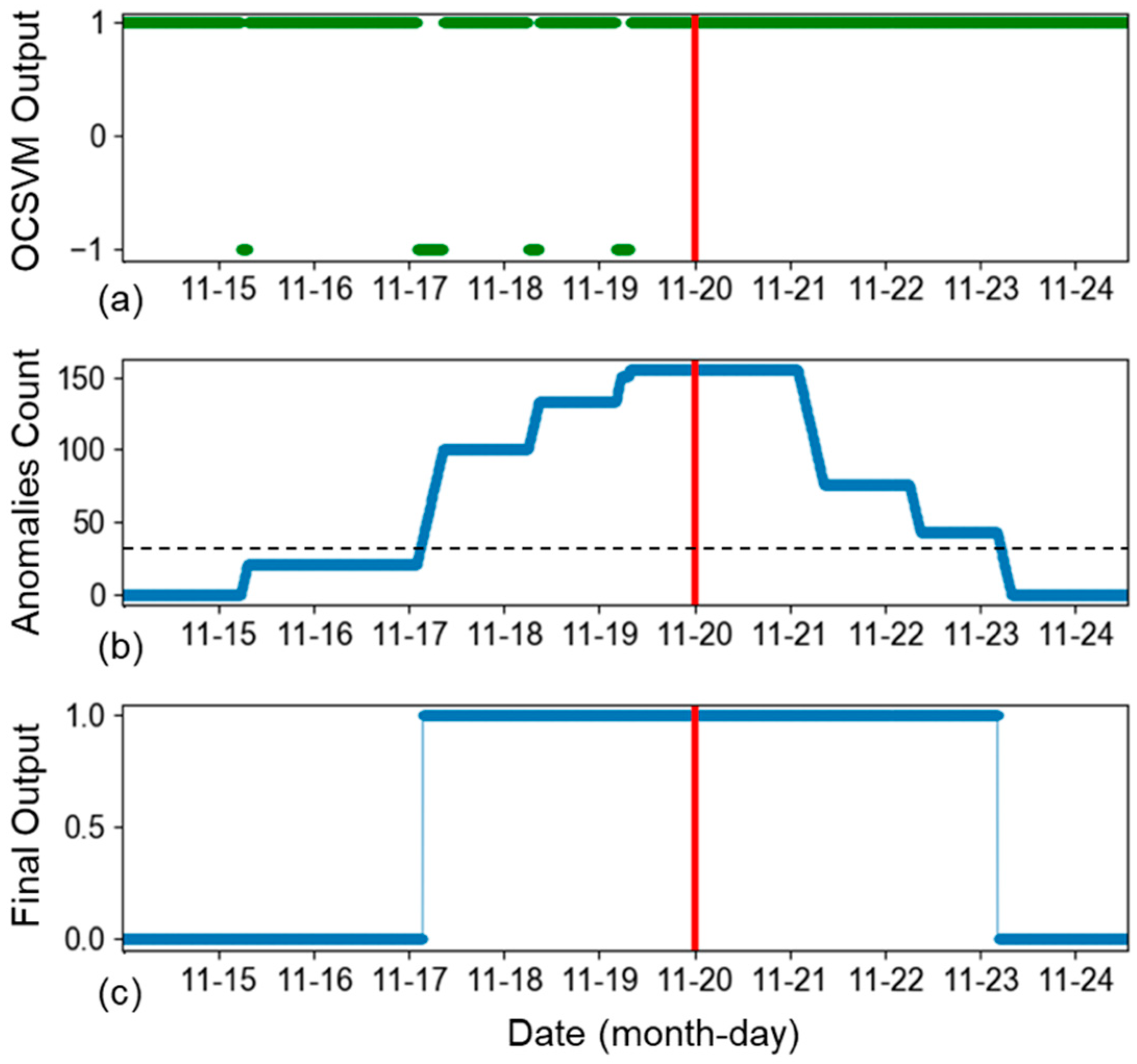
A preliminary analysis of the OCSVM model highlighted an unstable output, identifying a high number of sparse anomalous observations (Figure 7a).

This particular behaviour, which was mainly due to the complexity of the underlying phenomenon, presents the following issues:

• Considering a visual representation for supporting maintenance operators, the output is not enough intuitive for a consistent interpretation;
• Considering model performance evaluation, the output cannot be directly exploited for the computation of the performance measures.

Thus, a different solution is proposed in this work and consists of an output refinement process defined by two modules:

• Anomalous Observations Count module: a new signal is generated by counting the number of anomalous observations predicted in a fixed time window (four days) preceding the prediction; output from this module is depicted in Figure 7b;
• Thresholding module: applying a threshold (dotted line in Figure 7b) on the output of the latter module, a new binary output (anomalous/normal status) is derived (Figure 7c). The final output is now stable and representative of an anomaly occurrence and can be easily interpreted by both an operator and an automatic system.

Since through the first module a time window which keeps in memory the number of anomalous observations that occurred in the past days was applied, the signal required some time before it dropped against to zero. Due to this behaviour, the anomaly event could last until after the maintenance action was completed, as depicted in Figure 7b,c. Moreover, since observations corresponding to maintenance interventions were not removed from the data, the anomaly persistence, after the failure report, could be due to a maintenance action on the asset, which generates a new anomaly event.

Therefore, the proposed approach consists of the development of a final model, referred to as global model, which is built in three steps (OCSVM, Anomalous Observations Count, and thresholding module) and it is characterized by three different parameters ($\nu$, $\gamma$, and threshold) for each involved track circuit. In other words, the global model is fitted to the $n$ track circuits selected for the study obtaining $n$ different models, which differ by the value of their parameters estimated through the analysis of the data of each specific track circuit.

More in detail, with the aim of selecting the best global model for each track circuit (i.e., tuning the global model free parameters), all the data on track circuits’ parameters of 2018 were used for the model selection, considering also the failures that occurred in the considered period. The range of the hyper-parameters tested for the OCSVM module was $\nu \in \left[0.01,0.02,0.05,0.1\right]$, $\gamma$ was tested in a logarithmic distributed space of 60 instances ranging from ${10}^{-6}$ to ${10}^3$, while the thresholds were tested in a range from 1% to 99% (normalized on the maximum value of anomalous observations count found on the validation set). The model was developed using Python and the learning, validation, and testing processes were performed in the Hitachi Rail STS laboratory in a Hadoop environment, exploiting Spark Framework (the selected environment is a copy of the one operative on the field).

Regarding the system configuration modeling, it was performed at plant level, considering a Bayesian Network (BN) model [74], using the outcomes of the anomaly detection model to set the prior probability. A BN is defined as the 2-tuple $\mathrm{BN}=\left\{\mathrm{P},\mathrm{G}\right\},$ where $\mathrm{P}$ is the set of the prior and conditioned probabilities and $\mathrm{G}$ represents a Directed Acyclic Graph (DAG) that models the network structure. The nodes are divided into parent nodes and child nodes: the parent nodes are those with outgoing arrows, while the child nodes present incoming arrows from the parent nodes.

Each node (indicated by a capital letter) is characterized by a stochastic variable that represents the probability that the node is in a state $a_i$ or in another. Conditional Probabilities (CP) express the causal relationship among the nodes, evaluated as the probability,

$$\mathbb{P}\left(a_i|b_j, c_k\right)=\mathbb{P}\left(A=a_i|B=b_j,C=c_k\right),$$

(3)

that the node $A$ is in $a_i$, given that $B$ is in $b_j$, $C$ is in $c_k$, and so on. The Prior Probabilities (PP) indicate the probabilities of being in a certain state for the nodes without parents (root nodes) that are independent from all the other nodes.

The probability that the node $A$ is in the state $a_i$ is evaluated as follows:

$$\mathbb{P}\left(a_i\right)={{\displaystyle \sum }}_{\forall b_j, \forall c_k}\mathbb{P}\left(a_i|b_j, c_k\right)\mathbb{P}\left(b_j, c_k\right),$$

(4)

where $\mathbb{P}\left(b_j, c_k\right)=\mathbb{P}\left(B=b_j,C=c_k\right)$ is the joint probability that $B$ is in $b_j$, $C$ is in $c_k$.

Applying the Bayesian Network approach, if the failure probabilities of the components are known and the functional relationships between the different levels of the system are identified, the failure probability of the superior levels and the reliability of the overall plant can be evaluated. Moreover, the Bayesian Network can be updated every time new information on the track circuit status becomes available from the anomaly detection model, providing deep and updated knowledge on plant behaviour. In this way, the criticality of each track circuit is estimated as the consequence that its failure would have on the other system’s components.

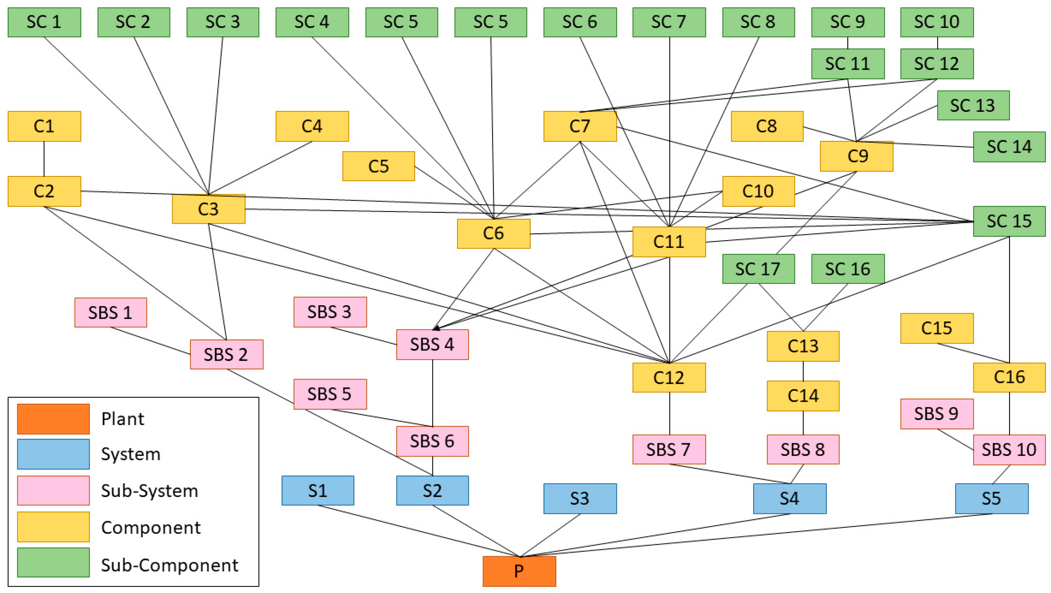
Three phases were considered in building the Bayesian Network in Figure 8, defined as the descriptive phase, structural phase, and relational phase.

The descriptive phase defines the system breakdown structure, that is, the system subdivision, into standardized levels: plant, system, subsystem, component, and subcomponent.

The structural phase identifies the root nodes and their prior failure probabilities (PP). Moreover, it involves the definition of the functional relationships between the elements of each level. The prior probabilities of the root nodes are derived by the data analytics results.

The relational phase evaluates the Conditional Probabilities for each child node and the posterior conditional failure probabilities (PCP) for each level. Then, the reliability of the plant is computed, given the prior failure probability of the root nodes and the conditional probability of each child node. In this way, the criticality of the track circuit in terms of impact on the overall system is determined.

Finally, the optimization was performed considering a risk-based scheduling model that allowed planning of the maintenance activities via a Mixed Integer Linear Programming (MILP) problem [75]. In the MILP problem the failure probability and the criticality of each track circuit, evaluated through the Bayesian Network, were then used to prioritize the interventions. As mentioned, the signaling system is a fail-safe system, since the safety of trains operation is always guaranteed even if a track circuit’s failure occurs, because the track section is automatically reported as occupied. Nevertheless, the false occupancy is a critical failure for rail operations since it has relevant consequences for trains’ circulation, usually implying the interruption of the service. Therefore, the optimization model took into account the risk of service disruptions, which was estimated by considering the criticality of the track circuit and its condition. The criticality was evaluated by applying the Bayesian Network approach, as the impact that a failure would have on the operation of the rail line. The status of track circuit was instead provided by the data-driven model.

In order to consider the risk in the decision-making process, the risk of a track circuit failure was considered in the objective function as a weight $r_i$, as described in Equation (5):

$$\min {\alpha }_1\left({{\displaystyle \sum }}_{i=1}^{\left|\mathcal{A}\right|}{r}_i{q}_i+{{\displaystyle \sum }}_{m=1}^{\left|\mathcal{T}\right|}{{\displaystyle \sum }}_{i=1}^{\left|\mathcal{A}\right|}{r}_i{c}_{i,m}\right)+{\alpha }_2{{\displaystyle \sum }}_{m=1}^{\left|\mathcal{T}\right|}{P}_m+{\alpha }_3{{\displaystyle \sum }}_{m=1}^{\left|\mathcal{T}\right|}{{\displaystyle \sum }}_{\begin{array}{c}g=1,\\ g\ne m\end{array}}^{\left|\mathcal{T}\right|}{\left(\mathsf{\Delta }{P}_{m,g}+\mathsf{\Delta }{N}_{m,g}\right)}_{,}$$

(5)

where:

• ${\alpha }_j$ is the importance of the $j^{t\mathrm{h}}$ term of the objective function, defined by the decision-maker;
• $r_i$ is the risk of failure of track circuit $i$;
• $c_{i,m}$ is the time needed to conclude the maintenance activity on the track circuit $i$ $\in \mathcal{A}$ executed by the maintenance crew $m$;
• $q_i$ is the difference between the planned time of execution and the expected one according to the criticality order;
• $P_m$ is the total path length covered by the maintenance crew $m\in \mathcal{T}$;
• $\mathsf{\Delta }{P}_{m,g}$ is the difference of the path lengths covered by the maintenance crews $m$ and $g$;
• $\mathsf{\Delta }{N}_{m,g}$ is the difference of the number of maintenance activities allocated to maintenance crews $m$ and $g$.

The optimization model made it possible to schedule the maintenance interventions in a sustainable way, taking into account different aspects related to sustainability. In particular, the optimization model considered track circuits’ status and criticality, preventing false track occupancies events and thus minimizing the risk of service disruptions. This implies a reduction of corrective maintenance activities that represent high costs for the infrastructure manager and for the society. Moreover, the model evaluated the optimal use of resources (maintenance crews), balancing the workload of each crew and guaranteeing the minimization of the covered distance to reach the assets to be maintained. To do this, the position of each track circuit along the line was considered, as well as the time needed for the crews’ movements.

Finally, the available time for maintenance was taken into account, evaluating the best allocation of maintenance activities to the available time windows; that is, those intervals during which the train circulation was stopped.

The optimization problem considered real operational constraints of the rail environment, such as the time and resources limitation. These limitations became mathematical constraints, expressed according to the formulation provided by Consilvio et al. [75].

Therefore, the efficiency and the sustainability of the maintenance process were pursued, avoiding unnecessary interventions and preventing failures. The benefit is the limitation of corrective maintenance activities and the reduction of the needed time for maintenance execution.

It is worth mentioning another important feature of the Decision Support System, that is, its capability of dealing with the uncertainty. Since real-world operational scenarios are characterized by a high level of uncertainty and unexpected events may occur at any time, the planning model is able to adapt its results in a dynamic way, in different situations. In particular, the optimization model updated the maintenance plan, when updated inputs and information regarding the track circuits’ status are provided by the data-driven model, or when an alarm is detected.

Moreover, since the anomaly detection is characterized by a given uncertainty, which is evaluated and reported in the Results section, the Decision Support System took into account this uncertainty, by considering the sensitivity of the solution to this variability.

Other adaptations of the previously defined maintenance plan were computed in case of delays of maintenance execution or unexpected unavailability of resources.

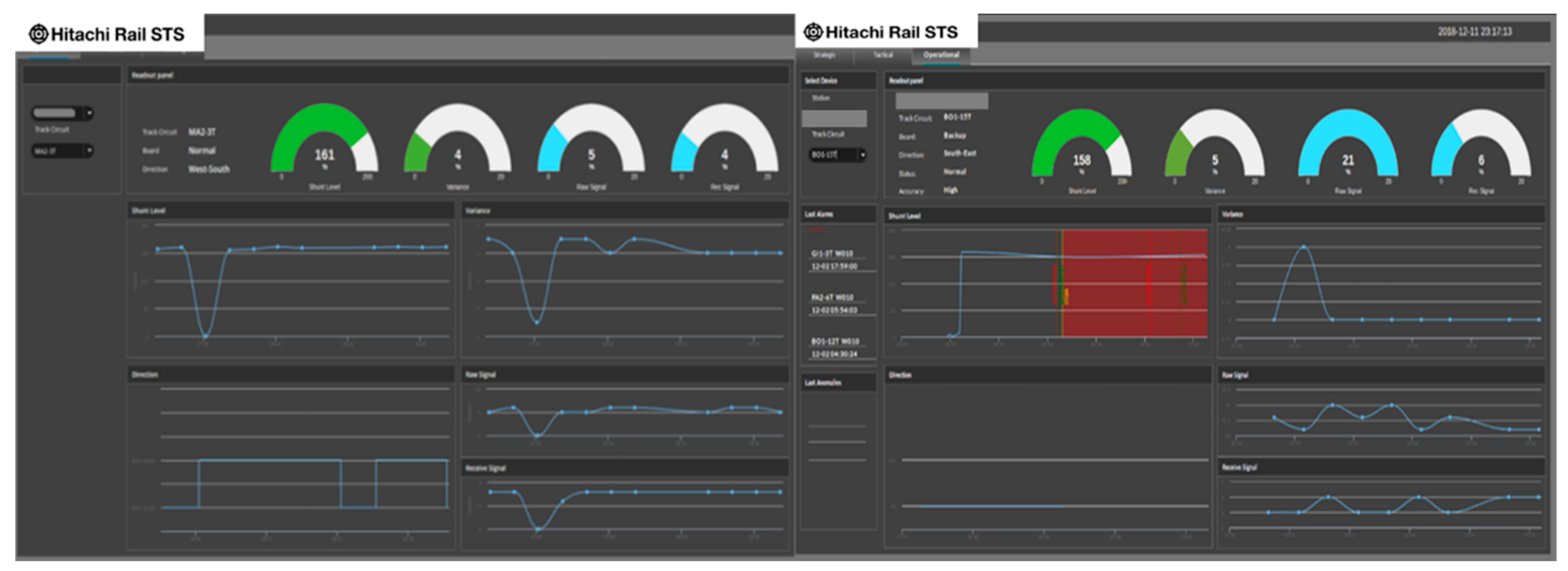
Regarding the output visualization, an HMI was developed to support the operators.

In Figure 9, the dashboard is represented with the information regarding the variation over time of the track circuits’ parameters and the anomaly detection. Moreover, a schematic view of the line is provided to the user that can select the station and the track circuit to be visualized.

6. Results

6.1. Case Study A: An Intelligent Asset Management System for Rail Earthworks

In this case study, the validation of the anomaly detection method, developed by applying the k-means algorithm, was performed. The objective of this data-driven approach was to highlight the precursors of earthwork failures and rapid degradation.

The KPIs, chosen to evaluate the goodness of the algorithm results, were the Silhouette coefficient (Si) (internal metric) and the Meila’s variation index (VI) (external metric). The Silhouette coefficient measures how much an object $i$ is similar to the other objects in its own cluster versus those in the neighbor cluster. The Meila’s variation index measures how the results of a cluster analysis fit an externally known result, such as externally provided class labels.

The earthwork cohorts chosen for the demonstration were defined considering track sections whose geometry had suffered a deterioration, and which lay in soil cuttings with an initial EHC in C. For these cohorts, the track geometry top and alignment standard deviation, the daily mean rainfall, and the mean earthwork soil moisture index (SMI) were the clustered variables. The application of the machine learning methodology provided the results shown in

Table 6. Data analytics key performance indicators (KPIs).

KPI Description	Percentage Improvement
Silhouette Coefficient (Si)	22%
Meila’s Variation Index (VI)	2%

.

The results show how the improvement related to the internal metric was much higher than the external metric one, as the computation of the KPI tends to be more independent of the internal layout of the cluster.

Regarding the validation of the decision-support model based on Petri nets, it was performed in comparison to SCAnNeR. SCAnNER is the current strategic decision support tool for EWs used by Network Rail, the U.K. Infrastructure Manager, which is based on Markov chains [79,80]. The aim was to prove that the proposed IAMS is able to provide output as reliable as SCAnNeR and, furthermore, to demonstrate that this modeling structure enables certain capabilities that SCAnNeR does not currently cover, such as the following:

• Improved granularity of the model, i.e., capability to model smaller groups or cohorts;
• Asset tracking;
• Higher versatility related to other factors such as examinations, restrictions, or degradation paths.

The validation was executed using two generic scenarios, where the outcomes from both algorithms were compared. The two scenarios were set considering a population of 70,000 soil cuttings, starting at time zero in earthwork condition (EHC) A. The first scenario (S1) considered the degradation of earthworks and their corrective renewal in F (failure). The second scenario (S2) considered an intervention mix with the following probabilities of intervention: (i) 10% of the assets are maintained in condition B; (ii) 10% of the assets are refurbished in condition C; (iii) 10% of the assets are renewed in condition D; (iv) 10% of the assets are refurbished and 10% are renewed in condition E; and (v) 100% of the assets that fail are immediately renewed.

The two models were compared using two different sources to compute the distributions in the transitions of the PN model. First of all, the lengths of the time steps and the degradation relationships used in the Petri net simulation were equivalent to those used in the Markov model, SCAnNeR. As a second analysis, tailor-made data-driven time distributions and probabilities for the PN model were used.

The objective of the validation was to have results with percentage differences between 5% and 10%.

Table 7. Validation of the PN model against SCAnNeR using the mean relative absolute error between their results.

Transition Source	Scenario	Mean Relative Absolute Error (%)
		EHC	Interventions
Markov	S1	2.60	5.50
Markov	S2	1.70	4.42
Data-driven	S1	N.A.	7.49

presents the results from the validation and how this objective was achieved. In the last case, using data-driven transitions, the comparison PN-SCAnNeR was not applicable, as the used time-steps are very different.

6.2. Case Study B: Track Circuits—False Track Occupancies Mitigation

The validation was conducted on 300 track circuits of an Italian rail line of 20 km, considering the data collected in the last two years. Moreover, the diagnostic and monitoring system of the track circuits has been upgraded in the last year to collect information with a high frequency, every five minutes (24 h).

To present the validation of the machine learning anomaly detection model, it is worth recalling the definition of anomaly. An anomaly is defined as the deviation of the reference parameter value from the nominal one. The anomaly is defined as a “real anomaly” if it is followed by a failure, otherwise it is called a “false anomaly”. In the considered case study, the failure consisted of a false occupancy of the track section.

Regarding the KPIs identified for the validation, they were the following:

• Anomaly detection precision, expressed as the ratio between the true anomalies and the total number of identified anomalies. It allowed the evaluation of the percentage of true anomalies, that is, anomalies that led to a failure (false track occupancy event). The total number of the identified anomalies was given by the sum of the real anomalies and the false anomalies, that is, those that did not lead to a false occupancy;
• True anomaly rate, which represented the capability of the anomaly detection model to anticipate false occupancy failures. It was expressed as the ratio between the true anomalies and all the occurred failures. It allowed the evaluation of the percentage of failures (false track occupancies) that were not anticipated by an anomaly identification;
• Time between the detection of the anomaly and the failure: difference between the timestamps of the two events (anomaly event raised by the system and occurred failure);
• Data processing from acquisition to HMI: that is, the time required for the whole data processing, from the raw data acquisition to the availability of the data on the HMI.

The obtained results are reported in

Table 8. Data analytics KPIs.

KPI Description	Obtained Results
Anomaly detection precision: true anomalies/identified anomalies	67%
True anomaly rate: true anomalies/all occurred failures	80%
Time between the detection of the anomaly and the failure	3.5 days
Data processing from acquisition to HMI	11 s

.

The maintenance planning model was validated in-lab trough the evaluation of other specific KPIs and the comparison with the current best-practice for preventive maintenance planning, applied in the considered rail line.

The KPI evaluation was performed according to the object function described in Equation (5), in which each term represents one of the following KPIs:

• Reduction of service disruptions risk: it was evaluated as the difference between the maintenance execution time, defined according to current best practice, and the execution time according to the plan defined by the DSS, considering asset status and criticality;
• Man-hour reduction: the man-hour reduction was computed as the decrease in time required by each team for completing the assigned maintenance activities. This allows a better exploitation of the train-free windows during which maintenance is performed. Comparing the results with the best practice scenario, a reduction of the total time for completing all the activities was obtained;
• Operator path optimization: the consideration of the path length in the cost function made it possible to find a solution that guarantees short distances covered by each maintenance team. The improvement was evaluated by comparing the optimized solution with the path length covered according to the current maintenance plan;
• Balance of maintenance team’s workload. This was evaluated by comparing the workload of the different maintenance crews. In particular, the number of the maintenance activities executed by each crew and the covered paths length was evaluated and compared in the current best practice scenario and in the scenario suggested by the DSS.

It is worth mentioning that these KPIs are strictly related to the sustainability of the maintenance process, as mentioned in Section 5.

In

Table 9. Decision Support System KPIs.

KPI Description	Obtained Results
Reduction of service disruptions’ risk	15 %
Man-hour reduction	17%
Operators’ path length reduction	7%
Increase of the balance of maintenance team’s workload	26%

, the results of the validation are provided.

The in-field implementation is currently under development within the In2Smart2 project to reach a TRL6/7, considering the application to an Italian metro line, specifically Milan Metro driverless Line 5, equipped with Hitachi Rail STS signalling system.

7. Conclusions

The main objective of the generic framework presented in this study was to guide the conception of Decision Support Systems focused on maintenance and interventions planning for railway infrastructure.

Machine learning and simulative techniques were applied, within the generic framework developed by the In2Smart Shift2Rail project, in order to build the DSS modules, considering different assets and techniques.

The applicability of the framework was demonstrated with two case studies: the “earthworks asset management case study” at the strategic level, and the “track circuits maintenance case study” at the tactical/operational level.

The framework was proven to be a useful guide for building a DSS for rail asset management. The main benefits of this approach are, among others:

• the possibility of taking into account the desired targets and KPIs of the decision-maker;
• the adaptability to different kinds of asset management problems;
• the modularity of the framework building blocks;
• the continuous performance monitoring of the overall asset management process.

Moreover, the proposed techniques to implement the framework were tested in a laboratory environment reaching TRL4 and the relevant results have been reported, showing the steps moved from risk-based condition-based maintenance towards predictive and prescriptive maintenance strategies.

The framework and the presented methodologies are currently under in-field implementation within the project, IN2SMART2, in order to reach a TRL 6/7.

References

1. Kandler, U.; Simroth, A.; et al. Common Understanding of the IAMS Process and Guiding Principles, Deliverable 9.1, s.l., In2Smart EU project, 2018.
2. Consilvio, A.; Crovetto, C.; Guyot, B.; Kirwan, A.; Mazzino, N.; Papa, F. Towards an intelligent and automated platform for railway Asset Management. In Proceedings of the 7th Transport Research Arena, TRA 2018, Vienna, Austria, 16–19 April 2018. [Google Scholar]
3. López-Campos, M.A.; Crespo Márquez, A. A Maintenance Management Framework Based on PAS 55. In Advanced Maintenance Modeling for Asset Management; Crespo Márquez, A., González-Prida Díaz, V., Gómez Fernández, J., Eds.; Springer: Cham, Switzerland, 2018. [Google Scholar]
4. Hanski, J.; Ojanen, V. Sustainability in strategic asset management frameworks: A systematic literature review. Int. J. Strateg. Eng. Asset Manag. 2020, accepted/in press. [Google Scholar]
5. Mjörnell, K.; Boss, A.; Lindahl, M.; Molnar, S. A Tool to Evaluate Different Renovation Alternatives with Regard to Sustainability. Sustainability 2014, 6, 4227–4245. [Google Scholar] [CrossRef] [Green Version]
6. Lee, S.-H.; Park, S.; Kim, J.M. Suggestion for a Framework for a Sustainable Infrastructure Asset Management Manual in Korea. Sustainability 2015, 7, 15003–15028. [Google Scholar] [CrossRef] [Green Version]
7. Maletič, D.; Maletič, M.; Al-Najjar, B.; Gomišček, B. Development of a Model Linking Physical Asset Management to Sustainability Performance: An Empirical Research. Sustainability 2018, 10, 4759. [Google Scholar] [CrossRef] [Green Version]
8. Franciosi, C.; Iung, B.; Miranda, S.; Riemma, S. Maintenance for Sustainability in the Industry 4.0 context: A Scoping Literature Review. IFAC-PapersOnLine 2018, 51, 903–908. [Google Scholar] [CrossRef]
9. Yang, Y.; Ng, S.T.; Xu, F.J.; Skitmore, M.; Zhou, S. Towards Resilient Civil Infrastructure Asset Management: An Information Elicitation and Analytical Framework. Sustainability 2019, 11, 4439. [Google Scholar] [CrossRef] [Green Version]
10. Sun, Y.; Ma, L.; Robinson, W.; Purser, M.; Mathew, A.; Fidge, C. Renewal Decision Support for Linear Assets. In Engineering Asset Management and Infrastructure Sustainability; Mathew, J., Ma, L., Tan, A., Weijnen, M., Eds.; Springer: London, UK, 2012. [Google Scholar]
11. Chen, Z.; Liang, Y.; Wu, Y.; Sun, L. Research on Comprehensive Multi-Infrastructure Optimization in Transportation Asset Management: The Case of Roads and Bridges. Sustainability 2019, 11, 4430. [Google Scholar] [CrossRef] [Green Version]
12. Kaewunruen, S.; Sresakoolchai, J.; Peng, J. Life Cycle Cost, Energy and Carbon Assessments of Beijing-Shanghai High-Speed Railway. Sustainability 2020, 12, 206. [Google Scholar] [CrossRef] [Green Version]
13. Rama, D.; Andrews, J.D. Railway infrastructure asset management: The whole-system life cost analysis. IET Intell. Transp. Syst. 2016, 10, 58–64. [Google Scholar] [CrossRef]
14. Armstrong, J.; Preston, J.; Hood, I. Adapting railways to provide resilience and sustainability. Proc. Inst. Civil Eng. Eng. Sustain. 2017, 170, 225–234. [Google Scholar] [CrossRef]
15. Niekamp, S.; Bharadwaj, U.R.; Sadhukhan, J.; Chryssanthopoulos, M.K. A multi-criteria decision support framework for sustainable asset management and challenges in its application. J. Ind. Prod. Eng. 2015, 32, 23–36. [Google Scholar] [CrossRef]
16. Lackhove, C.; Brinkmann, F.; Scheier, B.; Mbakwe, I.; Böhm, T. Advancing life-cycle-management for railway signalling and control systems. In Proceedings of the Towards Life Cycle Sustainability Management—LCM, Berlin, Germany, 28 August–1 September 2011. [Google Scholar]
17. Setrag, K.; Rostetter, C. Digital Prescriptive Maintenance. In Internet of Things, Process of Everything, BPM Everywhere; Amazon: Seattle, WA, USA, 2015; pp. 1–20. [Google Scholar]
18. Guillén, A.J.; Crespo, A.; Gómez, J.F.; Sanz, M.D. A framework for effective management of condition based maintenance programs in the context of industrial development of E-Maintenance strategies. Comput. Ind. 2016, 82, 170–185. [Google Scholar] [CrossRef]
19. Kour, R.; Tretten, P.; Karim, R. eMaintenance solution through online data analysis for railway maintenance decision-making. J. Qual. Maint. Eng. 2014, 20, 262–275. [Google Scholar] [CrossRef]
20. Thaduri, A.; Aljumaili, M.; Kour, R.; Karim, R. Cybersecurity for eMaintenance in railway infrastructure: Risks and consequences. Int. J. Syst. Assur. Eng. Manag. 2019, 10, 149. [Google Scholar] [CrossRef] [Green Version]
21. Asplund, M.; Famurewa, S.; Rantatalo, M. Condition monitoring and e-maintenance solution of railway wheels. J. Qual. Maint. Eng. 2014, 20, 216–232. [Google Scholar] [CrossRef]
22. Attoh-Okine, N. Big data challenges in railway engineering. In Proceedings of the 2014 IEEE International Conference on Big Data (Big Data), Washington, DC, USA, 27–30 October 2014; pp. 7–9. [Google Scholar]
23. Morris, C.; Easton, J.; Roberts, C. Applications of linked data in the rail domain. In Proceedings of the IEEE International Conference on Big Data, Washington, DC, USA, 27–30 October 2014; pp. 35–41. [Google Scholar]
24. Zarembski, A.M. Some examples of big data in railroad engineering. In Proceedings of the 2014 IEEE International Conference on Big Data (Big Data), Washington, DC, USA, 27–30 October 2014; pp. 96–102. [Google Scholar]
25. Spigolon, R.; Oneto, L.; Anastasovski, D.; Fabrizio, N.; Swiatek, M.; Canepa, R.; Anguita, D. Improving Railway Maintenance Actions with Big Data and Distributed Ledger Technologies. In INNS Big Data and Deep Learning (INNSBDDL); Springer: Cham, Switzerland, 2019. [Google Scholar]
26. Izquierdo, J.; Crespo Márquez, A.; Uribetxebarria, J. Dynamic artificial neural network-based reliability considering operational context of assets. Reliab. Eng. Syst. Saf. 2019, 188, 483–493. [Google Scholar] [CrossRef]
27. Carvalho, T.P.; Soares, F.A.; Vita, R.; Francisco, R.D.P.; Basto, J.P.; Alcalá, S.G. A systematic literature review of machine learning methods applied to predictive maintenance. Comput. Ind. Eng. 2019, 137, 106024. [Google Scholar] [CrossRef]
28. Karim, R.; Westerberg, J.; Galar, D.; Kumar, U. Maintenance Analytics—The New Know in Maintenance. IFAC-PapersOnLine 2016, 49, 214–219. [Google Scholar] [CrossRef]
29. Ghofrani, F.; He, Q.; Goverde, R.M.P.; Liu, X. Recent applications of big data analytics in railway transportation systems: A survey. Transp. Res. Part C Emerg. Technol. 2018, 90, 226–246. [Google Scholar] [CrossRef]
30. Thaduri, A.; Galar, D.; Kumar, U. Railway assets: A potential domain for big data analytics. Procedia Comput. Sci. 2015, 53, 457–467. [Google Scholar] [CrossRef] [Green Version]
31. Pipe, K.; Culkin, B. An automated data-driven toolset for predictive analytics. In Proceedings of the 7th IET Conference on Railway Condition Monitoring 2016 (RCM 2016), Birmingham, UK, 27–28 September 2016; pp. 1–7. [Google Scholar]
32. Lee, T.; Tso, M. A universal sensor data platform modelled for realtime asset condition surveillance and big data analytics for railway systems: Developing a “Smart Railway” mastermind for the betterment of reliability, availability, maintainbility and safety of railway systems and passenger service. In Proceedings of the 2016 IEEE SENSORS, Orlando, FL, USA, 30 October–3 November 2016; pp. 1–3. [Google Scholar]
33. Morant, A.; Larsson-Kråik, P.O.; Kumar, U. Data-driven model for maintenance decision support—A case study of railway signalling systems. Proc. Inst. Mech. Eng. Part F 2016, 230, 220–234. [Google Scholar] [CrossRef] [Green Version]
34. Yang, L.; Xu, T.; Wang, Z. Agent based heterogeneous data integration and maintenance decision support for high-speed railway signal system. In Proceedings of the 17th International IEEE Conference on Intelligent Transportation Systems (ITSC), Qingdao, China, 8–11 October 2014; pp. 1976–1981. [Google Scholar]
35. Núñez, A.; Hendriks, J.; Li, Z.; De Schutter, B.; Dollevoet, R. Facilitating maintenance decisions on the Dutch railways using big data: The ABA case study. In Proceedings of the IEEE International Conference on Big Data (Big Data), Washington, DC, USA, 27–30 October 2014; pp. 48–53. [Google Scholar]
36. Jamshidi, A.; Hajizadeh, S.; Su, Z.; Naeimi, M.; Núñez, A.; Dollevoet, R.; De Schutter, B.; Li, Z. A decision support approach for condition-based maintenance of rails based on big data analysis. Transp. Res. Part C Emerg. Technol. 2018, 95, 185–206. [Google Scholar] [CrossRef] [Green Version]
37. Consilvio, A.; Iorani, M.; Iovane, V.; Sciutto, M.; Sciutto, G. Real-time monitoring of the longitudinal strain of continuous welded rail for safety improvement. Proc. IMechE Part F J. Rail Rapid Transit 2019, 1–15. [Google Scholar] [CrossRef]
38. Aivaliotis, P.; Georgoulias, K.; Arkouli, Z.; Makris, S. Methodology for enabling Digital Twin using advanced physics-based modeling in predictive maintenance. Procedia CIRP 2019, 81, 417–422. [Google Scholar] [CrossRef]
39. Galar, D.; Thaduri, A.; Catelani, M.; Ciani, L. Context awareness for maintenance decision-making: A diagnosis and prognosis approach. Measurement 2015, 67, 137–150. [Google Scholar] [CrossRef]
40. Vathoopan, M.; Johny, M.; Zoitl, A.; Knoll, A. Modular Fault Ascription and Corrective Maintenance Using a Digital Twin. IFAC-PapersOnLine 2018, 51, 1041–1046. [Google Scholar] [CrossRef]
41. Kaewunruen, S.; Xu, N. Digital Twin for Sustainability Evaluation of Railway Station Buildings. Front. Built Environ. 2018, 4, 77. [Google Scholar] [CrossRef] [Green Version]
42. Guillen, A.J.; Crespo, A.; Gómez, J.; González-Prida, V.; Kobbacy, K.; Shariff, S. Building Information Modeling as Assest Management Tool. IFAC-PapersOnLine 2016, 49, 191–196. [Google Scholar] [CrossRef]
43. Aivaliotis, P.; Georgoulias, K.; Chryssolouris, G. The use of Digital Twin for predictive maintenance in manufacturing. Int. J. Comput. Integr. Manuf. 2019, 32, 1067–1080. [Google Scholar] [CrossRef]
44. Kritzinger, W.; Karner, M.; Traar, G.; Henjes, J.; Sihn, W. Digital Twin in manufacturing: A categorical literature review and classification. IFAC-PapersOnLine 2018, 51, 1016–1022. [Google Scholar] [CrossRef]
45. Kivits, R.A.; Furneaux, C. BIM: Enabling Sustainability and Asset Management through Knowledge Management. Sci. World J. 2013, 14. [Google Scholar] [CrossRef]
46. Kaewunruen, S.; Lian, Q. Digital twin aided sustainability-based lifecycle management for railway turnout systems. J. Clean. Prod. 2019, 228, 1537–1551. [Google Scholar] [CrossRef]
47. Neves, J.; Sampaio, Z.; Vilela, M. A Case Study of BIM Implementation in Rail Track Rehabilitation. Infrastructures 2019, 4, 8. [Google Scholar] [CrossRef] [Green Version]
48. Baglietto, E.; Consilvio, A.; Di Febbraro, A.; Papa, F.; Sacco, N. A Bayesian Network approach for the reliability analysis of complex railway systems. In Proceedings of the 2018 International Conference on Intelligent Rail Transportation (ICIRT), Singapore, 12–14 December 2018; pp. 1–6. [Google Scholar]
49. Colla, I.; Consilvio, A.; Olmi, A.; Romano, A.; Sciutto, M. High Density—HD Using ERTMS: The Italian Solution for the Railway Traffic Management. In Proceedings of the 2018 IEEE International Conference on Environment and Electrical Engineering and 2018 IEEE Industrial and Commercial Power Systems Europe (EEEIC/I&CPS Europe), Palermo, Italy, 12–15 June 2018; pp. 1–6. [Google Scholar]
50. Di Febbraro, A.; Giglio, D.; Sacco, N. On analyzing the vulnerabilities of a railway network with Petri nets. Transp. Res. Procedia 2017, 27, 553–560. [Google Scholar] [CrossRef]
51. Rama, D.; Andrews, J. A Holistic Approach to Railway Infrastructure Asset Management. Int. J. Perform. Eng. 2015, 2, 107–120. [Google Scholar]
52. Andrews, J. A modeling approach to railway track asset management. Proc. Inst. Mech. Eng. Part F 2013, 227, 56–73. [Google Scholar] [CrossRef]
53. Shang, H.; Beŕenguer, C. Delayed Maintenance Model for Deteriorating Track Using Colored Petri Nets. IFAC-PapersOnLine 2015, 48, 464–469. [Google Scholar] [CrossRef]
54. Le, B.; Andrews, J.; Fecarotti, C. A Petri net model for railway bridge maintenance. Proc. Inst. Mech. Eng. Part O 2017, 231, 306–323. [Google Scholar] [CrossRef]
55. Liang, C.; Ghazel, M.; Cazier, O.; El-Koursi, E. Risk analysis on level crossings using a causal bayesian network based approach. Transp. Res. Procedia 2017, 25, 2167–2181. [Google Scholar] [CrossRef]
56. Jiang, L.; Wang, X.; Liu, Y. Reliability assessment of ZPW-2000A track circuit using bayesian network. In Proceedings of the 11th International Conference on Reliability, Maintainability and Safety (ICRMS), Hangzhou, China, 26–28 October 2016; pp. 1–4. [Google Scholar]
57. Baigen, C.; Bin, C.; Wei, S.; Jian, W.; Jiang, L.; Debiao, L.; Wei, J. Real-time reliability evaluation method for train-ground communication subsystem based on dynamic bayesian networks. In Proceedings of the International Conference on Electromagnetics in Advanced Applications (ICEAA), Cairns, QLD, Australia, 19–23 September 2016; pp. 556–559. [Google Scholar]
58. Rodič, B. Industry 4.0 and the New Simulation Modeling Paradigm. Organizacija 2017, 50, 193–207. [Google Scholar] [CrossRef] [Green Version]
59. Márquez, A.C.; Del Castillo, A.C.; Gómez Fernández, J.F. Integrating artificial intelligent techniques and continuous time simulation modeling. Practical predictive analytics for energy efficiency and failure detection. Comput. Ind. 2020, 115, 103164. [Google Scholar] [CrossRef]
60. Consilvio, A.; Di Febbraro, A.; Sacco, N. A modular model to schedule predictive railway maintenance operations. In Proceedings of the International Conference on Models and Technologies for Intelligent Transportation Systems (MT-ITS), Budapest, Hungary, 3–5 June 2015; pp. 426–433. [Google Scholar]
61. Faris, M.; Núñez, A.; Su, Z.; De Schutter, B. Distributed Optimization for Railway Track Maintenance Operations Planning. In Proceedings of the 21st International Conference on Intelligent Transportation Systems (ITSC), Maui, HI, USA, 4–7 November 2018; pp. 1194–1201. [Google Scholar]
62. D’Ariano, A.; Meng, L.; Centulio, G.; Corman, F. Integrated stochastic optimization approaches for tactical scheduling of trains and railway infrastructure maintenance. Comput. Ind. Eng. 2019, 127, 1315–1335. [Google Scholar] [CrossRef]
63. Andrews, J.; Prescott, D.; De Rozières, F. A stochastic model for railway track asset management. Reliab. Eng. Syst. Saf. 2014, 130, 76–84. [Google Scholar] [CrossRef]
64. Baldi, M.; Heinicke, F.; Simroth, A.; Tadei, R. New heuristics for the Stochastic Tactical Railway Maintenance Problem. Omega 2016, 63, 94–102. [Google Scholar] [CrossRef] [Green Version]
65. Consilvio, A.; Di Febbraro, A.; Sacco, N. Stochastic scheduling approach for predictive risk-based railway maintenance. In Proceedings of the IEEE International Conference on Intelligent Rail Transportation (ICIRT), Birmingham, UK, 23–25 August 2016; pp. 197–203. [Google Scholar]
66. Jiménez-Redondo, N.; Mingolarra-Garaizar, I. et al. Generic Framework for Decision Support Systems in Maintenance and Interventions Planning. Deliverable 9.2., s.l., IN2SMART EU Project, 2019.
67. ISO. ISO 55000: 2014 Preview Asset Management—Overview, Principles and Terminology, s.l.: ISO; ISO: Geneva, Switzerland, 2014. [Google Scholar]
68. UIC. Railway Application Guide: Practical Implementation of Asset Management through ISO 55000; Union Internationale des Chemins de fer: Paris, France, 2016. [Google Scholar]
69. Saxena, A.; Prasad, M.; Gupta, A.; Bharill, N.; Prakash Patel, O.; Tiwari, A.; Joo Er, M.; Ding, W.; Lin, C.T. A review of clustering techniques and developments. Neurocomputing 2017, 267, 664–681. [Google Scholar] [CrossRef] [Green Version]
70. Murata, T. Petri nets: Properties, analysis and applications. Proc. IEEE 1989, 77, 541–580. [Google Scholar] [CrossRef]
71. Raychaudhuri, S. Introduction to Monte Carlo simulation. In Proceedings of the 2008 Winter Simulation Conference, Miami, FL, USA, 7–10 December 2008; pp. 91–100. [Google Scholar]
72. Schölkopf, B.; Smola, A.; Müller, K.R. Nonlinear Component Analysis as a Kernel Eigenvalue Problem. Neural Comput. 1998, 10, 1299–1319. [Google Scholar] [CrossRef] [Green Version]
73. Cortes, C.; Vapnik, V. Support-vector networks. Mach. Learn. 1995, 20, 273–297. [Google Scholar] [CrossRef]
74. Heckerman, D.; Breese, J.S. Causal independence for probability assessment and inference using Bayesian networks. IEEE Trans. Syst. Man Cybern. Part A 1996, 26, 826–831. [Google Scholar] [CrossRef] [Green Version]
75. Consilvio, A.; Di Febbraro, A.; Meo, R.; Sacco, N. Risk-based optimal scheduling of maintenance activities in a railway network. EURO J. Transp. Logist. 2019, 8, 435–465. [Google Scholar] [CrossRef]
76. Bornia, O.; Vignola, G. et al. Anomalies Detection Approaches and Use Cases; Deliverable 8.1, s.l. In2Smart EU Project, 2018.
77. Bornia, O.; Vignola, G. et al. Anomalies Detection Prototype and Validation Report; Deliverable 8.2, s.l. In2Smart EU Project, 2019.
78. Consilvio, A.; Sanetti, P.; Anguita, D.; Crovetto, C.; Dambra, C.; Oneto, L.; Papa, F.; Sacco, N. Prescriptive maintenance of railway infrastructure: From data analytics to decision support. In Proceedings of the 6th International Conference on Models and Technologies for Intelligent Transport Systems, Kraków, Poland, 5–7 June 2019; pp. 1–10. [Google Scholar]
79. Network Rail. Earthworks Technical Strategy. Safety, Technical and Engineering; Network Rail: Milton Keynes, UK, 2018. [Google Scholar]
80. Power, C.; Mian, J.; Spink, T.; Abbott, S.; Edwards, M. Development of an evidence-based geotechnical asset management policy for Network Rail, Great Britain. Procedia Eng. 2016, 143, 726–733. [Google Scholar] [CrossRef] [Green Version]
Figure 1. The general framework.
Sustainability 12 02544 g001
Figure 2. Decision Support System (DSS) elements and interactions.
Sustainability 12 02544 g002
Figure 3. Two-dimensional cluster analysis of earthworks conditions (EHC).
Sustainability 12 02544 g003
Figure 4. Basic element of the Petri nets (PN) model.
Sustainability 12 02544 g004
Figure 5. Petri net model for the soil cutting cohort.
Sustainability 12 02544 g005
Figure 6. Human–machine interface HMI graphical output visualization (Risk and Condition Scores are dimensionless).
Sustainability 12 02544 g006
Figure 7. Model refinement steps from raw output of One-class Support Vector Machine (OCSVM) (a) to stable final output (c); the red vertical line represents a failure occurrence, while the dotted horizontal line in (b) represents the threshold exploited in the process.
Sustainability 12 02544 g007
Figure 8. System configuration—Bayesian Network.
Sustainability 12 02544 g008
Figure 9. HMI dashboard: comparison of track circuits in nominal and out-of-range conditions (detection of anomaly in red).
Sustainability 12 02544 g009