Uncertainty Analysis for Data-Driven Chance-Constrained Optimization

Abstract

In this contribution our developed framework for data-driven chance-constrained optimization is extended with an uncertainty analysis module. The module quantifies uncertainty in output variables of rigorous simulations. It chooses the most accurate parametric continuous probability distribution model, minimizing deviation between model and data. A constraint is added to favour less complex models with a minimal required quality regarding the fit. The bases of the module are over 100 probability distribution models provided in the Scipy package in Python, a rigorous case-study is conducted selecting the four most relevant models for the application at hand. The applicability and precision of the uncertainty analyser module is investigated for an impact factor calculation in life cycle impact assessment to quantify the uncertainty in the results. Furthermore, the extended framework is verified with data from a first principle process model of a chloralkali plant, demonstrating the increased precision of the uncertainty description of the output variables, resulting in 25% increase in accuracy in the chance-constraint calculation.

1. Introduction

Environmental sustainability has grown to become a more pressing subject for the chemical industry. A clear indicator is the joining of forces of the major industry representatives: VCI (association of the German chemical industry), IG BCE (industry union of mining, chemistry and energy) and BAVC (chemistry federation of employers), to set common sustainability goals for the German chemical industry. These goals among other things include development of more sustainable processes [1].

The growing interest in more sustainable processes has led to a renewed interest in process systems engineering. PSE provides optimization and decision-making tools, which can be used in the chemical industry to reduce its environmental impact [2]. The area of application can range from equipment optimisation to optimising entire supply-chains, both during the conceptual phase and operations.

Linking environmental aspects with the optimization tools provided by PSE requires accurate models describing the environmental impacts, the economics of the process, and the process operation [3]. These can be implemented in multiobjective optimization formulations, where the environmental description is incorporated either as an objective or as a constraint. A method where these models have been linked successfully for optimization purposes is the process to planet (P2P) method. P2P combines complex nonlinear process models with life cycle assessment (LCA) models and evironmentally extended input–output (EEIO) models [4]. It is vital when using environmental models, such as LCA models, in decision making schemes to account for the uncertainty arising due to in instance model simplifications or parameterization [5]. Many decision making schemes follow the threshold-concept, i.e., defining a value for an environmental descriptor, above which it is considered to be harmful. The decision schemes can therefore only be applicable if they are combined with a statistical analysis [6].

The additional uncertainty in environmental models mostly relate to parameters derived in LCA [7]. The uncertainty can be subdivided into parameter uncertainty due to imprecise knowledge or life cycle inventory (LCI) and life cycle impact assessment (LCIA) parameters, temporal and spatial variability in LCI and LCIA parameters, variability between sources in the LCI, variability between sources between objects of assessment in the LCIA, uncertainty in models and uncertainty in choices [8]. Due to the manifold of superposing uncertainties in LCA, the parametric distribution is assumed to be non-normally distributed [5]. Additionally, non-normal distributions are found in the environmental model outputs [9] and nonlinear process models. There are a wide variety of methods to analyse and quantify uncertainty in LCA models [10,11]. While the ISO standard for LCA acknowledges that uncertainty analysis is still in its infancy, [11] with sensitivity analysis being the most commonly used method [12], more complex methods have recently been published. These methods include uncertainty analysis methods such as Monte Carlo and Latin Hyper Cube sampling [13] or Fuzzy programming [14]. Consequently, combining environmental models and process models in optimization, referred to as sustainable optimization, must always consider uncertainty [15]. There are three different methods to include uncertainty in optimization. Stochastic programming with recourse, robust optimization and chance-constrained optimization [2]. In this study we focus on chance-constrained optimization, in line with previous works at our department [16,17].

PSE provides methods for both offline and real-time optimization, while real-time optimization has a greater potential for more accurate and flexible process operations [18]. Using chance-constrained optimization for real-time applications would enable the incorporation of environmental models with highly uncertain parameters and still achieve accurate online computation of optimal and stable process operating conditions. However, for rigorous non-linear models existing chance-constrained optimization frameworks result in computational times from a couple of hours to several days, not allowing for online application [17].

Therefore, a new framework for chance-constrained optimization has been developed at the department, decreasing the computational effort significantly. This is achieved by exchanging rigorous models for the optimization with data-driven ones. Uncertainty is included in additional data-driven models. The data-driven models are trained on the variance of the output variables for data-sets subjected to uncertainty. The uncertainty in the data is generated by sampling the rigorous models with parameters subjected to uncertainty, for which a probability distribution might be known. However, modelling of uncertainty in the model outputs in the current framework is limited up to now to normal distributions [16].

The complex distribution shape of environmental model parameters and its outputs [9] can not be sufficiently described by a normal distribution. This leads to large deviations in the probability calculations and the expected output values. By consequence, this leads to erroneous results in chance-constrained optimization.

There are a multitude of uncertainty analysis methods, the choice depends on the source and form of uncertainty as well as the area and precision of application [10]. For the application at hand where the uncertainty information is statistical and need to remain numerical for the desicion making scheme a uncertainty analysis method which bases on Monte Carlo sampling is the only relevant possibility.

To allow for the implementation of environmental models in chance-constrained optimization, an adaptive approach is studied to improve the uncertainty modelling. Implementing more complex distribution functions to model the uncertainty while keeping the computational effort at a minimum.

It is therefore the aim of this paper to develop and implement a method to improve uncertainty modelling for data-driven chance-constrained optimization. By using more complex probability distribution functions while keeping the computational effort at a minimum. This would allow the implementation of environmental models coupled with process models for real-time optimization.

2. Methods

Combining rigorous non-linear process models with environmental models containing highly uncertain parameters for real-time optimization, requires: (1) A stable and precise method for optimization under uncertainty [19], (2) a framework with a computational time allowing for real-time application [16] and (3) an accurate uncertainty modelling framework, quantifying the distribution for a wide variety of probability distribution shapes.

2.1. Optimization under Uncertainty

Chance-constrained optimization, as an approach to include uncertainty in optimization problems, in general relies on physiochemical models. The underlying non-linear system contains parameters subjected to uncertainty [17]. These parameters will in the following be referred to as uncertain parameters. Uncertainty is included by enforcing a predefined probability for the fulfilment of inequality constraints [19]. A well-developed approach is a sequential approach (single shooting) with the probability calculation included as an additional layer to map the inequality constraints to the uncertain parameter space [20]. The elaborate probability calculation is the most computationally intensive part of the optimization. The computational time ranges from a couple of hours to several days [17].

2.2. Data-Driven Chance-Constrained Optimization Framework

To eliminate the computational limitation of conventional chance-constrained optimization frameworks, a data-driven chance-constrained optimization framework was developed. It decreases the computational effort compared to earlier frameworks. This is achieved by exchanging the rigorous models with data-driven ones. Additionally, using a data-driven uncertainty model, which maps the uncertainty of the outputs over the input space, reduces the computationally effort for the probability calculation significantly [16].

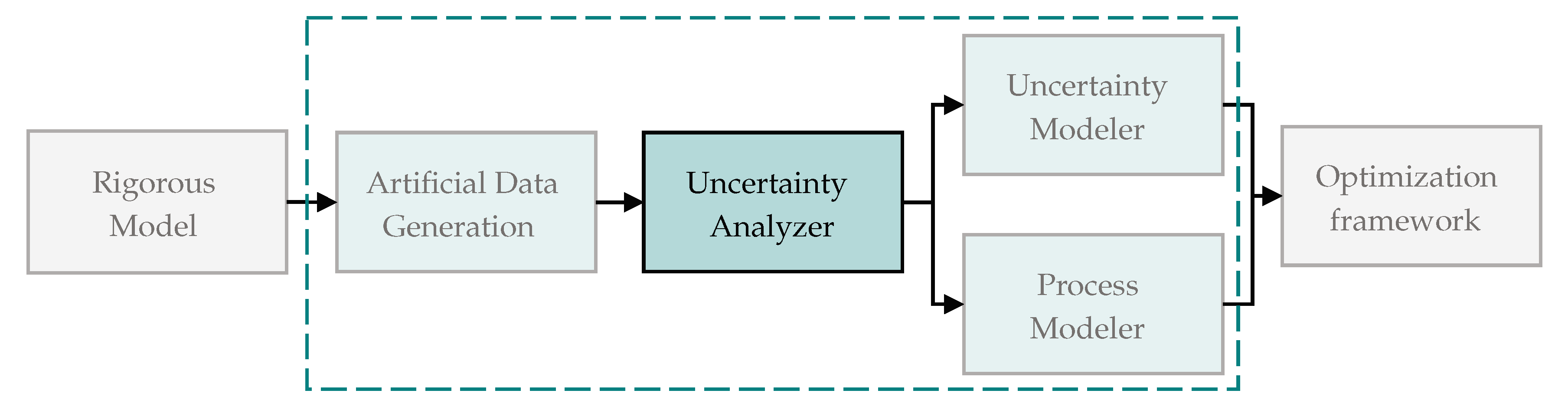
The generation of the data-driven process and uncertainty models (DDPUM) is conducted offline in an upstream framework, implemented in Python. The data-driven models are subsequently inserted in the chance-constrained optimization framework. The DDPUM generation can be separated into three steps beginning with the sampling of a rigorous model and ending with the training of data-driven input–output and uncertainty models. The workflow is shown schematically in Figure 1:

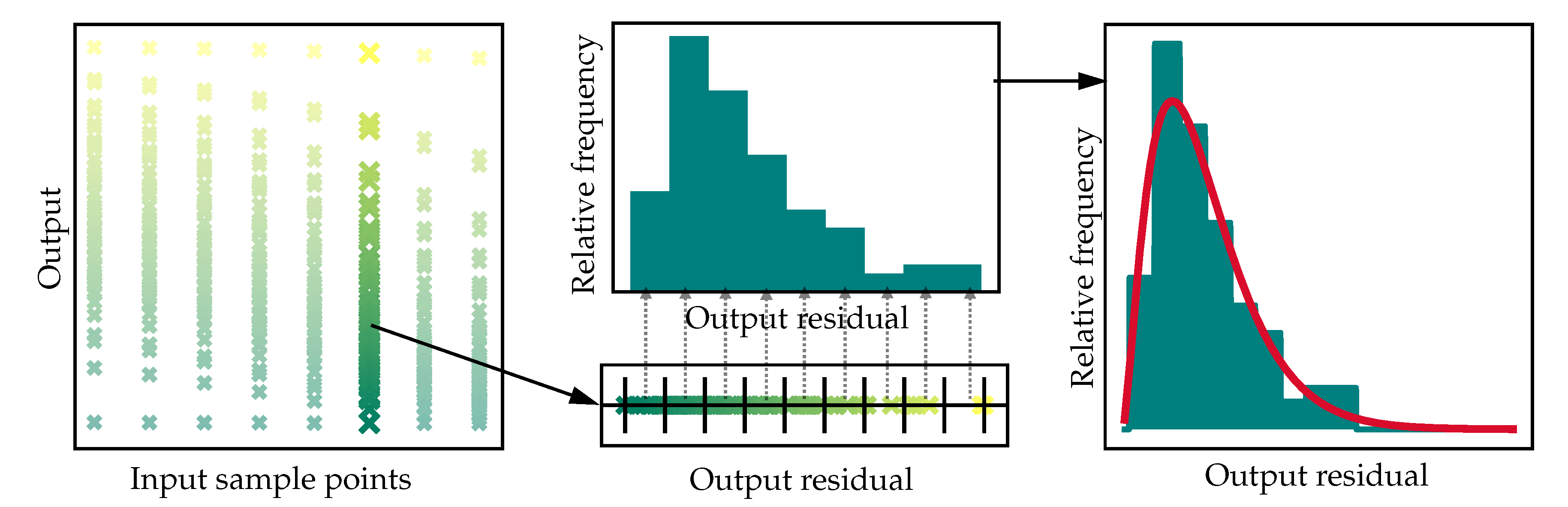
During the artificial data generation, the design variables of the rigorous model are divided into input variables and parameters. The space of input variables defines the boundaries, within which the data-driven models will be valid. Some of the model parameters might be subject to uncertainty with either known or unknown probability distributions. The probability distribution of every uncertain parameter must be specified. The parameter space contains the distribution of the uncertain parameters. Both spaces are sampled to create a high-density data-set, this is visualised for one input and one output variable in the left plot in Figure 3. The artificial data is generated by solving the rigorous model for each input and parameter combination using AMPL [21] or MatLab.

The second step is the analysis of the uncertainty. Therein, the uncertain outputs at every input point are analysed and a probability distribution function is fitted to the data. The resulting probability distribution parameters and the expected values at every point in the input space are used in the subsequent modelling steps. Until now the quantification of uncertainty is limited to normal distributions. This may lead to large deviations when modelling uncertainty generated from environmental models with non-normally distributed parameters or non-linear process models.

The third step is the generation of the data-driven process models. An input–output model is generated based on the expected values of the output variables from the previous step. The uncertainty model is trained on the probability distribution model parameters. The uncertainty can vary for each point in the input space and output space.

Finally, the data-driven models can be introduced into chance-constrained optimization problems. In the approach presented in this contribution the probability can be calculated directly from the cumulative probability density function (CDF) described by the parameters returned from the data-driven uncertainty model. Therefore, avoiding elaborate multivariate integration. Hence enabling quick computation of expected values, probabilities, and gradients necessary for fast convergence of the optimization.

2.3. Uncertainty Analyser Framework

In this contribution an adaptive framework analysing and modelling uncertainty has been developed. The framework allows for the implementation of process models and environmental models in the DDPUM framework, with non-normally distributed output variables.

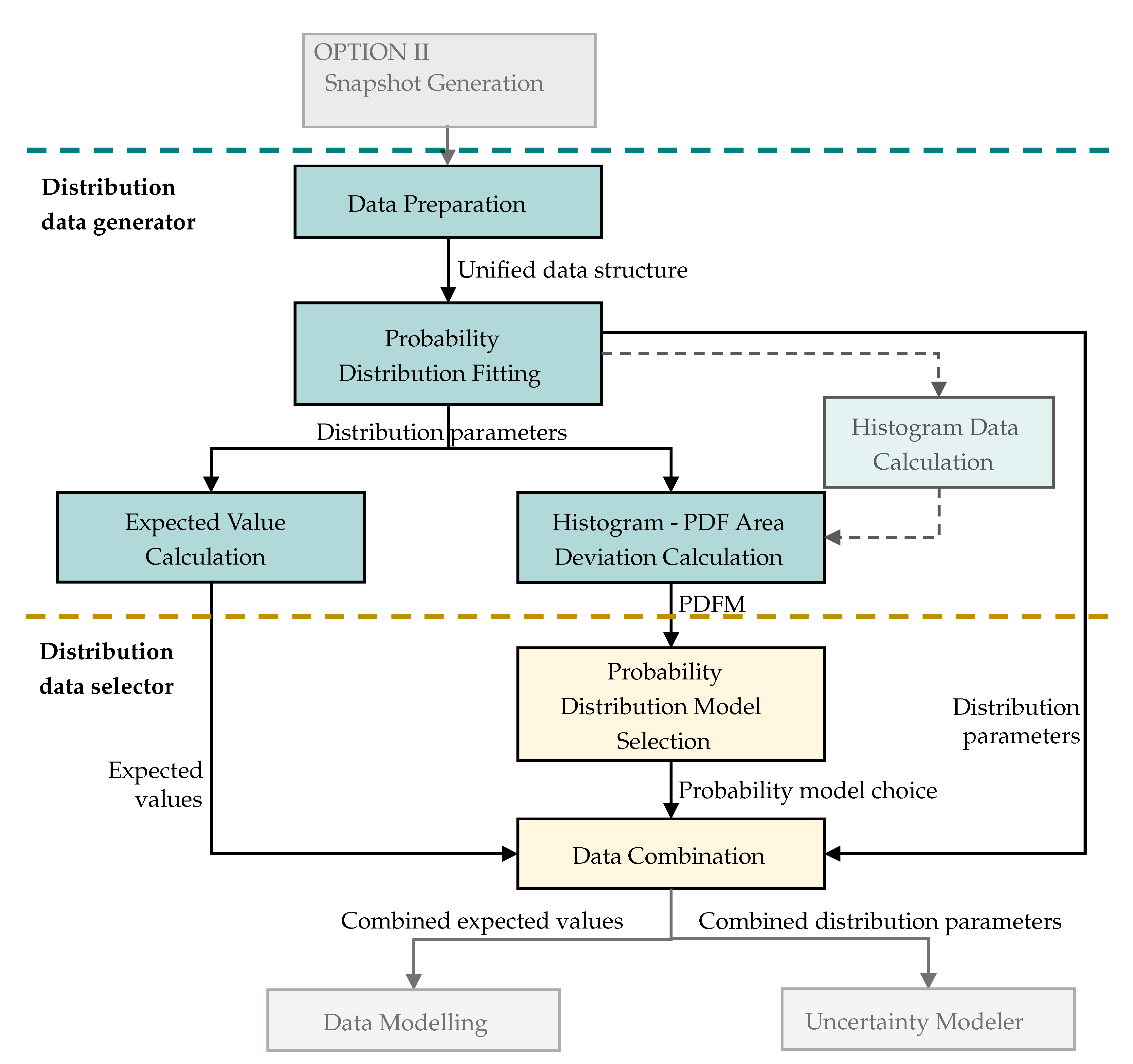
The framework is developed as a separate module in Python referred to as uncertainty modelling module (UMM). The UMM consists of two submodules which are called successively during the execution of the module. In Figure 2 the workflow of the UMM is displayed, the dashed lines mark the beginning of each submodule. The light gray arrows show how the UMM is connected to the rest of the data-driven DDPUM framework.

The distribution data generator (DDG) is the first submodule. It fits probability distribution models to the uncertainty data. The input of the module is artificial data from rigorous models, generated in the Artificial Data Generation step in the DDPUM framework. As seen in Figure 2 and visualized in the left plot in Figure 3, the execution of the DDG consists of four steps. The first step is the data preparation. It returns a uniform data structure, allowing different data types, as inputs, e.g., pickles, a file format used to store data in python, or mat files, a file format storing data from Matlab. Subsequently the uncertainty data in the artificial output-data is fitted with a continuous probability distribution model, specified when calling the submodule. The path from uncertain data in a model output to a probability distribution model fit is shown in Figure 3. The fitting returns the probability distribution model parameters, i.e., the scale, location, and shape parameters. The data is fitted with the statistical module provided by SciPy (scipy.stats) [22]. The fitting is carried out by maximizing the logarithmic likelihood function. This optimization problem does not necessarily lead to a globally optimal fit. [22]. Testing the framework for a variety of distributions has shown that the fits are sufficiently accurate for the application in hand. The UMM can fit the data with around 100 different probability distribution models. Based on an extensive case-study, presented in Section 3, to enhance the computational effort and considering the similarity of parametric probability distribution functions [23], the set of distribution functions is reduced to the four most accurate continuous probability distribution models for provided by SciPy for artificial data-sets including uncertainty.

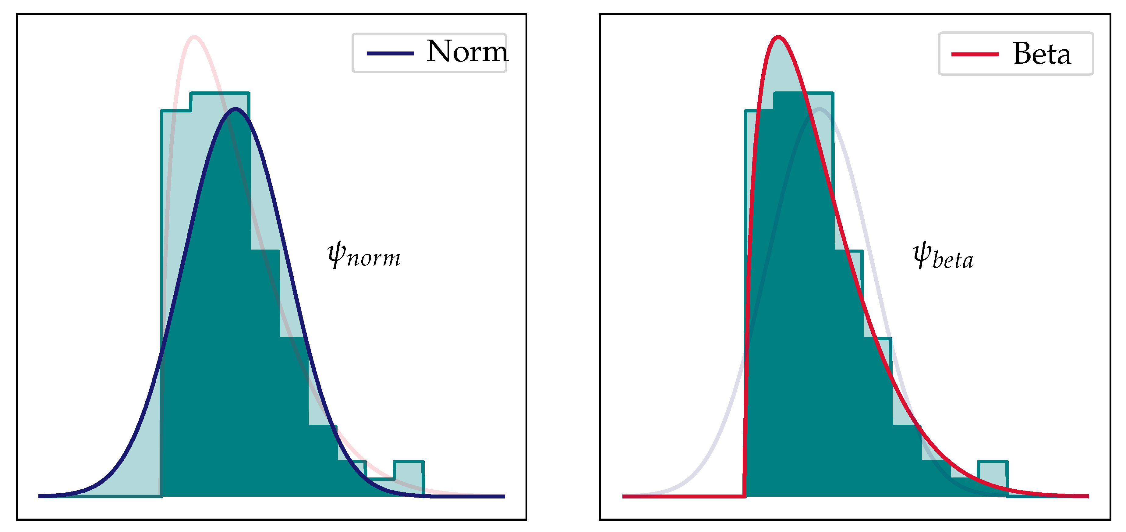
The third step is the evaluation of the fit of the probability distribution models. For this purpose, a metric is defined describing the deviation between model and data. The probability distribution fit metric (PDFM), $\psi$, is defined as the area between the histogram and the probability density function. The lower limiting case, with a sample size towards infinity and a perfect fit is $\psi \to 0$. In turn, the upper limiting case for a complete model mismatch is $\psi \to 1$. The PDFM is visualized for an arbitrary skewed distribution in Figure 4. Comparing the left and right plot, clearly shows that the beta distribution function with a smaller area between probability density function (PDF) and histogram, i.e., a lower PDFM-value, fits the uncertainty data better. In the fourth step the expected values are calculated with the distribution models fitted in the second step.

The second submodule, called distribution data selector (DDS) chooses the most accurate distribution functions returned by the DDG. For big sample sizes, for which a binominal distribution approaches a continuous distribution, the PDFM can be used directly to choose between probability distribution functions, since there will be a clear distribution to match. For smaller sample sizes a variation of the likelihood-ratio test is applied. The likelihood-ratio test chooses between two distribution models based on their maximum likelihood [24]. The PDFM is regarded as a definite fit-description of the probability distribution model, hence the ratio of the PDFMs will indicate, which probability distribution model describes the data better. Distribution functions with more shape parameters will in most cases have a more accurate fit [23]. Models with additional shape parameters will need more data-driven models in the uncertainty model step in the optimization framework. Leading to more computational effort for the optimizer. Therefore, a constraint is added to favour less complex models with a minimum required quality regarding the fit. Based on the PDFM-ratios and considering the constraint, a model is chosen. Finally, the distribution parameters and expected values are combined for all outputs based on their individual distribution model choice.

3. Uncertainty Analysis

Probability distribution of a model output can take on a variety of shapes, depending on the non-linearity of the model and the distribution shape of the uncertain parameters. There is a large number of continuous probability distribution models, though the number of models which have become prominent is relatively low [25]. Around 100 of of the most prominent continuous distribution models are implemented in scipy.stats [22]. This case study aims to find continuous probability distribution models, which can describe unimodal probability distribution shapes most accurately, weighting in the complexity of the model, represented by the number of shape parameters, and the computational effort of the model fitting. To evaluate the ability to fit of the models, a five step evaluation scheme is constructed, which is presented in Figure 5. The weights are chosen based on the commonness of the distribution shapes in chemical engineering applications.

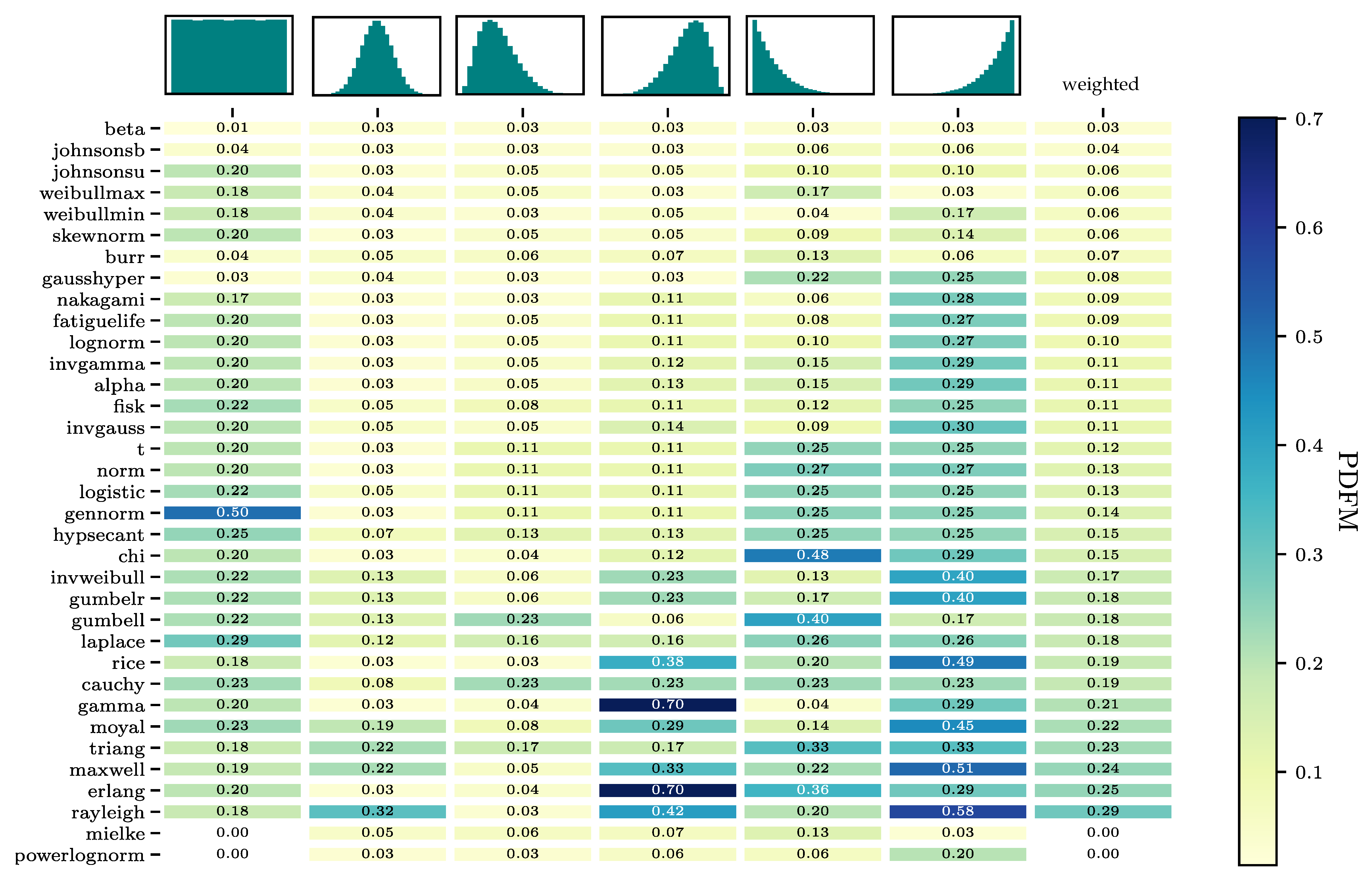
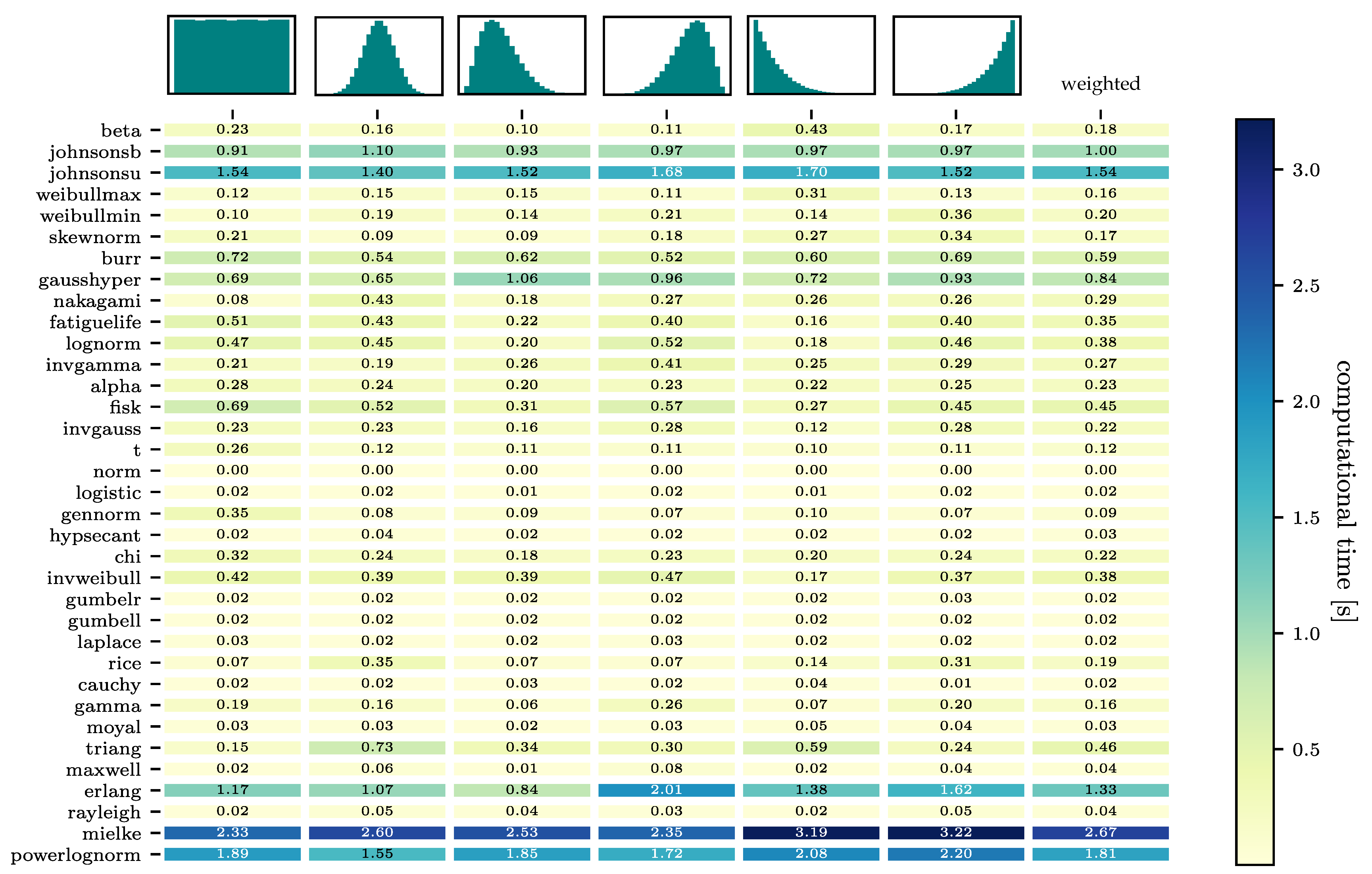
The 100 continuous distribution models in scipy.stats are reduced to a set of 40 distribution models in the first step due to their insufficient accuracy in modelling a normal distribution. The results concerning their ability to fit are shown Figure A1 and the weighted matrix of the computational times in Figure A2 in the Appendix A. The four distribution models with the highest weighted results concerning their ability to fit, equivalent to the first four models, i.e., rows in the heatmap, are: Beta, Johnsons b, Skewnorm, and Weibull max. All of them describe the normal and skewed distributions nearly error-free, seen by the low PDFM values in columns 1, 3, and 4. The PDFM values for the more uncommon distribution shapes, uniform and exponential, columns 2, 5, and 6, are also relatively low. The four models are divided into two sets, one set containing the models with two shape parameters (beta and the Johnsons b) and one set with the models containing only one shape parametes (Skewnorm and Weibull max). The computational effort of Johnsons b is almost twice as high as for the beta distribution. In the one-shape-parameter-set a difference in computational effort is not as evident. The Weibull max has a slightly lower computational effort, though the Skewnorm model shows a more balanced fit-quality for the right-left skewed and exponential increasing-decreasing shapes.

It can therefore be concluded, that the beta distribution is the best two-shape-parametric distribution model. For the one-parametric distribution model, both the Weilbull max and Skewnorm are well suited distribution models. The normalised probability density functions of the three probability distribution functions are shown in Equations (1)–(3), respectively [22].

$$\begin{array}{cc}\hfill f_{\beta }(x,a,b)& =\frac{\Gamma (a+b)·x^{a-1}{(1-x)}^{b-1}}{\Gamma \left(a\right)·\Gamma \left(b\right)}\hfill \end{array}$$

(1)

$$\begin{array}{cc}\hfill f_{w_{max}}(x,c)& =c·{(-x)}^{c-1}·exp\left(-{(-x)}^c\right)\hfill \end{array}$$

(2)

$$\begin{array}{cc}\hfill f_{skew-N}(x,d)& =\frac{1}{\sqrt{2\pi }}exp(-x^2/2)\left[1+\mathrm{erf}\left(\frac{d·x}{\sqrt{2}}\right)\right]\hfill \end{array}$$

(3)

3.1. Case Study: Applicability on LCIA with Uncertain Parameters

The best probability distribution models from the evaluation scheme are implemented in the uncertainty analyzer framework. The uncertainty analyzer framework is tested with a case study exemplifying the workflow and decision process in the uncertainty analysis. The case study is based on a life cycle impact assessment step, where the uncertainty of the calculated impact scores are analysed. In general this is equivalent to an uncertainty analysis of an output of a linear model with non-normal distributed uncertain parameters.

Since the models in LCA are parametric representations, the uncertainty in the model outputs is due to the uncertainty of the model parameters. The uncertainty of the model parameters must be analysed during the design and validation of the model. The thereby derived uncertainty information can either be qualitative or quantitative depending on the uncertainty analysis method chosen [10]. For data-driven chance-constrained optimization, the uncertainty information needs to be quantitative. Quantifying uncertainty is most commonly done with probability distribution models, where the complexity and the accuracy of the chosen probability distribution model depends on the quality of the distribution data for the uncertain parameters [26]. The presented uncertainty analyzer framework, does not estimate the probability distribution of the uncertain parameters, but uses this information to quantify and model the distribution of the outputs needed for the chance-constrained optimization.

In this case study the uncertainty in the impact score, W, is caused by uncertainty in the characterisation factor, $x_i$, and the component mass flow, $m_i$, for n components and is based on the uncertainty data derived by [5]. The uncertainty in the parameters was assessed heuristically and empirically, based on uncertainty due to imprecise knowledge or LCI and LCIA parameters, temporal and spatial variability in LCI and LCIA parameters, variability between sources in the LCI, variability between sources between objects of assessment in the LCIA, uncertainty in models, and uncertainty in choices [8].

Equation (4) shows how the impact factors are calculated considering a composition uncertainty and an uncertain characterization factor.

$$W=\sum _{i=1}^n{m}_i·x_i$$

(4)

The composition uncertainty of the component mass flow is assumed to be uniformly distributed, since the lower and upper bound are determined through a best and worst case scenario, respectively. The characterization factor is assumed to be right skewed and described by a log-normal probability distribution [5]. The distribution in the characterization factor is described by a dispersion factor, which determines the skewness of the distribution.

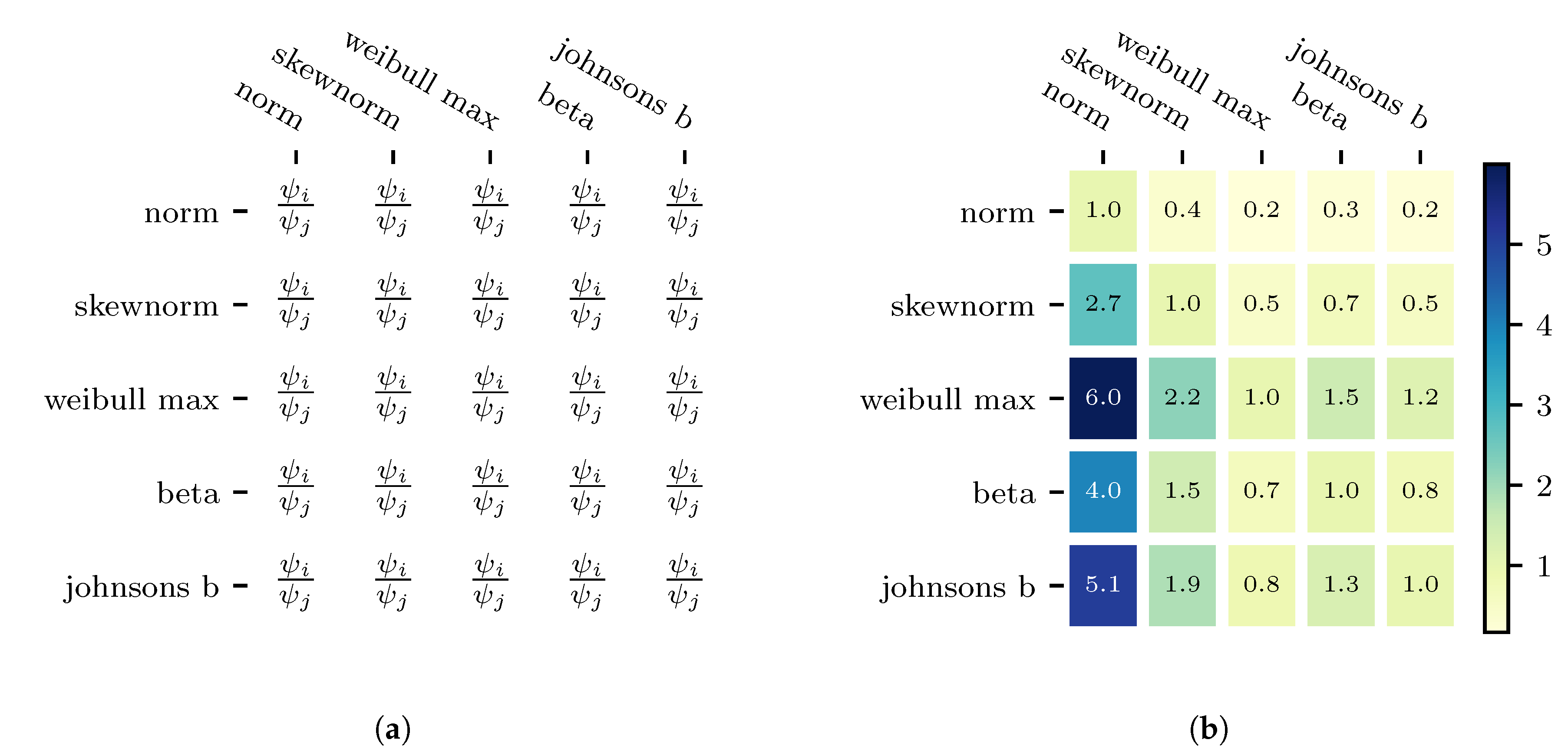
To test the uncertainty analyzer framework, an artificial data-set is created in the artificial data generation step of the DDPUM framework. The parameters are sampled two-dimensionally with a Hammersley sampling method, while the distribution of the parameters is specified with the lognormal and uniform probability distribution model provided by scipy.stats [22]. The model is solved in AMPL [21] and the uncertain impact factor data-set is passed on to the uncertainty analyser framework. The fit-accuracy of the five probability distribution models is calculated in the Probability Distribution Model Selection. The PDFM-ratio of the probability distribution models is shown in Figure 6a and with the corresponding values of the case study in Figure 6b.

From Figure 6b it can be derived that the third row, which corresponds to the weibull max probability distribution method, is the most accurate model. If the ratio equals one, then both models fit the distribution data equally well and the greater the value, the more accurate the fit. The complexity of probability distribution models, defined by the number of shape parameters, n, is taken into account by defining a significance level, $\alpha$. $\alpha$ is introduced to favour less complex probability distribution models, which result in fewer data-driven uncertainty models in the following DDPUM framework step. For the case study, a 5% significance level is chosen. Models with more shape parameters must therefore be $\Delta n·5\%$ more accurate than a model with less shape parameters with $\Delta n$ corresponding to the difference in shape parameters. The PDFM-ratios for Weibull max model are all greater than one and do not violate the constraint. It can therefore be concluded that the weibull max method is the most accurate probability distribution model to describe uncertainty in the impact factor.

Comparing the uncertainty analyser framework with the approach to model all outputs with a normal probability distribution model, reveals that the uncertainty analyser framework is up to six times more accurate. The comparison can be derived directly from the first column in Figure 6b, the values represent the deviation of the probability distribution of the normal distribution compared to Weibull Max (row 3).

3.2. Case Study: Improvement in the Chance Constraint Calculation for a Chlor-Alkali Process

The approach in the DDPUM-framework is to model the uncertainty with data-driven models. These data-driven models map the probability distribution model parameters of the model outputs over model inputs. This concept is only valid if the parameters returned by the data-driven uncertainty model can correctly reconstruct the uncertainty distribution in the model outputs. It can be argued, that all distribution function parameters are continuous and smooth over the variable space, since they, i.e., (location, scale, and shape parameters) have physical or geometrical properties ([25], p. 19). Smooth data-driven models should therefore be able to correctly model the probability distribution model parameters over the input variable space.

To test if the uncertainty description, i.e., the probability distribution model parameters, returned by the new uncertainty analyser framework can be used to accurately reconstruct the model output distributions, a rigorous model of an industrial chloralkali electrolyzer [16] is examined. Additionally, the accuracy of the uncertainty analysis of the old framework, where the uncertainty distribution in all model outputs is assumed to be normal, is compared to that of the new.

The model outputs used, are the chloride mass fraction and the anolyte brine flow at the outlet. The considered input variables are the current density and the anolyte brine feed flow. The current efficiency regarding sodium hydroxide is considered as uncertain parameter following a normal distribution. Sampling over the inputs and the parameters is carried out and for each combination of input and parameter, the rigorous model is solved using AMPL [21]. The dataset is passed on to the uncertainty analyser.

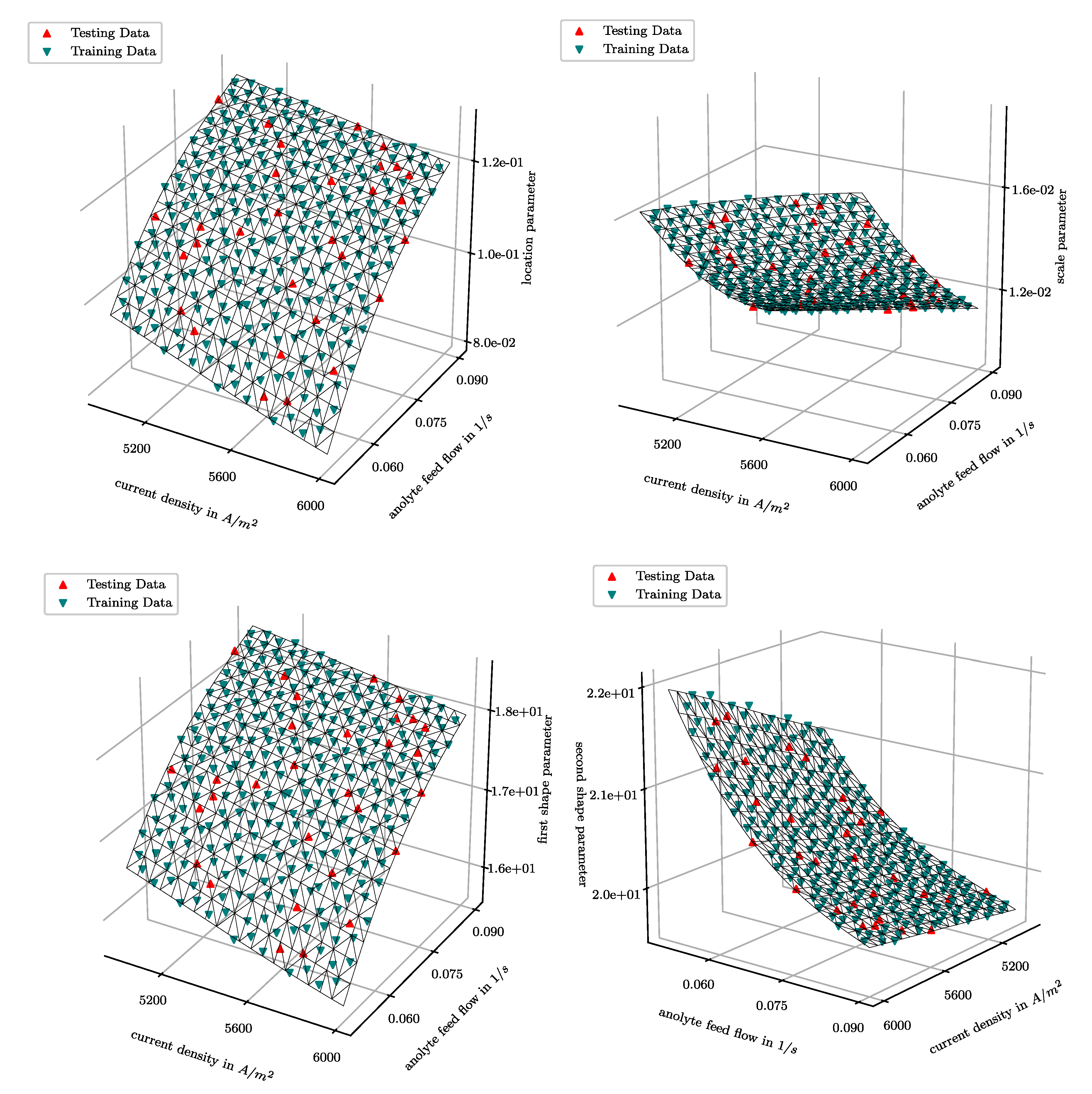
The uncertainty analyser selects the beta distribution model to describe the uncertainty in both outputs. For the generation of the data-driven distribution models a Gaussian process regression model is chosen. The model is trained with 90% of the uncertainty data, referred to as testing data, the remaining 10% of the data is used to test the predictability of the model. The model is both tested on the capability to correctly map the distribution parameters and on the accuracy of the predicted distributions, based on the testing data.

The results, presented in Figure 7, show a smooth curvature of the uncertainty model for all parameters. The fit of the Gaussian process regression model has a mean squared error of 5.0 × 10${}^{-6}$. and a percentile deviation of 0.043%. The low mean squared error and the percentile deviation of the data-driven model indicates that a data-driven model can map the distribution parameters over the input space accurately.

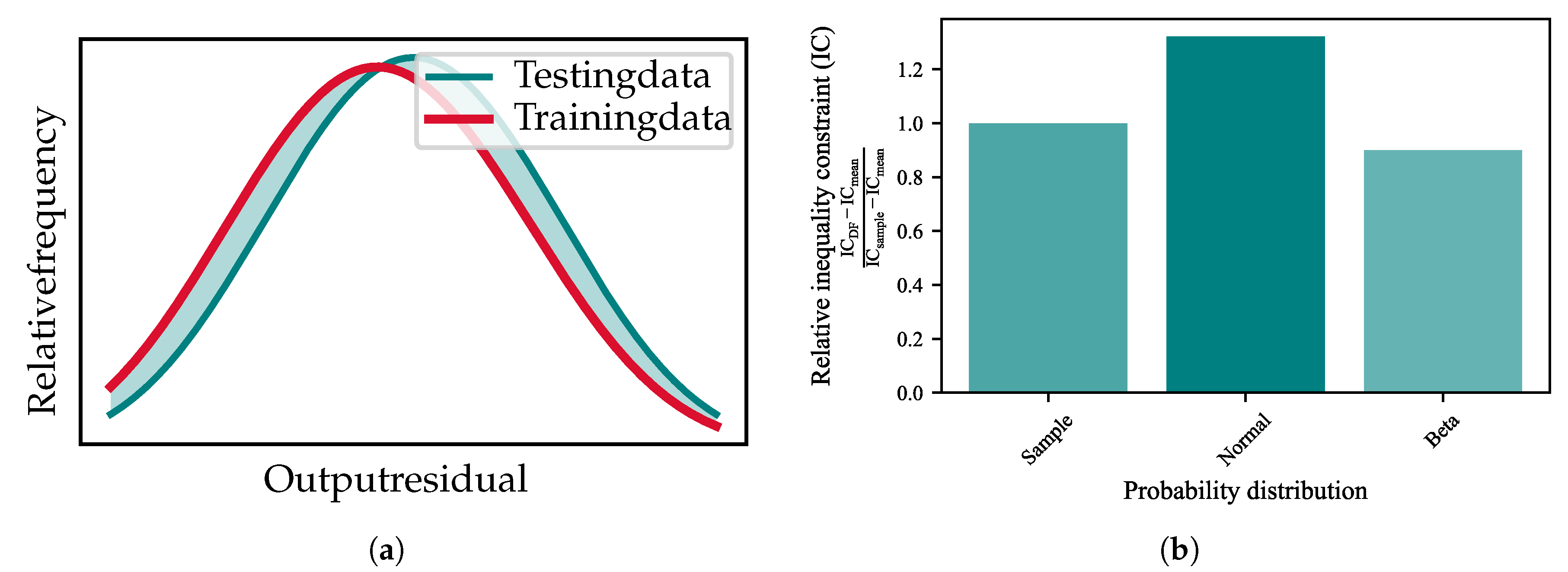
In addition to the fit quality of the data-driven model, it must be tested if the distribution parameters returned from the data-driven model correctly recreate the distribution of the output variables at each input-point. Therefore an additional fit-error parameter $\theta$, similar to the PDFM is introduced. It evaluates the deviation of the PDF modelled by the distribution function parameters of the testing data and the predicted PDFs at these points. The deviation equals the shaded area between the two PDFs, as shown in Figure 8a. $\theta$ is scaled between 0 and 1, where 0 is the case when the PDFs of the testing and training data overlap completely and 1 when there is no overlap. The resulting mean $\theta$ for all testing points in the data-set of this case study is 4.3 × 10${}^{-4}$. The low value in $\theta$ shows that the distribution parameters returned by the UM can correctly recreate the distribution of the output variables.

The accuracy of the new uncertainty analyser framework for chance-constrained optimization is compared to the former version. Therefore a reference data-driven uncertainty model is trained on the mean and variance of the model outputs, i.e., assuming a normal distribution. In data-driven chance-constrained optimization, the chance constraint is checked by calculating the probability of the inequality constraint using the parametric CDF with the distribution model parameters returned by the data-driven uncertainty model. The inequality constraints are chosen as model outputs, hence the accuracy of the chance constraint calculation can be evaluated directly with the data-driven uncertainty model. To test the accuracy of the chance constraint calculation, we firstly define the chance constraint level, which corresponds to the minimal probability level that the inequality constraint is satisfied. Secondly, we use the inverse function of the CDF, the percent point function (PPF), to calculate the maximal value of the inequality constraint to the set chance constraint. To have a reference value, when comparing the inequality constraints, the relative frequency of the sample data is used to estimate a value of the chance constraint. In this case study we consider the model output: Chloride mass fraction as an inequality constraint. The chloride mass fraction, to a cumulative probability of 99%, is calculated with the data-driven uncertainty model trained on the normal distribution parameters, with the data-driven model trained on the beta probability distribution model parameters and with the relative frequency of the sample data. To assess the relative improvement, the inequality constraints are subtracted by the mean value and divided by the value calculated with the relative frequency. The values calculated from the sample data directly are assumed to be close to the population statistic, i.e., the “real” value. When the sample size increases the results from the relative frequency approaches the population value. The results of the relative inequality constraint is shown in Figure 8b. The beta probability distribution model almost returns the exact inequality constraint, while If we use the normal distribution, the solution violates the inequality 25% of the time.

It is thus concluded that the uncertainty of the output variables can be fully and accurately modelled with a data-driven model mapping the distribution function parameters over the input space. While significantly improving the accuracy chance constraint evaluation in the data-driven chance-constrained optimization.

4. Conclusions

In this contribution, an extension of the framework for the generation of data-driven models for chance-constrained optimization, with an uncertainty analyser framework is presented. The uncertainty analyser framework can model sample data subjected to uncertainty with a wide variety of unimodal probability distribution models, choosing the most accurate probability distribution model by minimizing the deviation to the uncertain data. Additionally, a constraint is implemented that favours less complex models with a minimal required quality regarding the fit. The new uncertainty analyser results in more accurate descriptions of uncertainty in model outputs, consequently improving the chance constraint calculation, which is a central building block in data-driven chance-constrained optimization.

A case study is performed selecting the four most relevant probability distribution models for problems at hand: Skewnorm, Weibull max, beta and Johnsons b. These models are further evaluated in a case study aiming to describe uncertainty in the impact factor in LCIA. The impact factor is chosen as the model output and the uncertainty arises due to skewed and uniform distributed model parameters. Applying the new method results in an accurate description of uncertainty in the model outputs by selecting the most suitable probability distribution model with the minimal deviation to the uncertainty data.

To test the potential of the uncertainty analyser framework for data-driven chance-constrained optimization, a rigorous process model for a chlor-alkali process was sampled and a data-driven uncertainty model generated with the extended DDPUM framework. An excellent fit for the data-driven uncertainty model is achieved, indicated by the mean squared deviation of 5.0E-6 (0.043%) and a distribution fit-error, representing the deviation of the predicted PDF, of 4.3E-4. The improvement for data-driven chance-constrained optimization with the new uncertainty analyser is evaluated. For this purpose the relative inequality constraint, set as the chloride mass fraction in the model, is calculated for a specified chance constraint level. The calculation is conducted with the old method, assuming normal distribution, and with the new uncertainty analyser. The evaluation shows, that the result of the chance constraint calculation with the new uncertainty analyser framework is almost error free. While when using the old method based on a normal distribution, the solution violates the inequality 25% of the time.

The combination of the results for both case studies shows that the precision of the framework for the generation of data-driven models for chance-constrained optimization is not limited by the uncertainty modelling. Allowing the implementation of models with high uncertainty, as environmental models, in decision making schemes, such as data-driven chance-constrained optimization.

The uncertainty analyser framework is limited to modelling the distribution in the output variables with unimodal probability distribution models. Alternatively the probability distribution can be modelled using Kernel density estimation, additionally describing multimodal probability distributions. However, this exceeds the limit of the presented DDPUM framework. Additionally, the computational effort of the framework and its precision could be improved by an adaptive sampling method linking the uncertainty analyser with the artificial data generation step in the DDPUM framework.