Modeling the Socioeconomic Metabolism of End-of-Life Tires Using Structural Equations: A Brazilian Case Study

 , , and
Abstract
1. Introduction
| Nomenclature | |
| SEM | Socioeconomic Metabolism |
| ELTs | End-of-Life Tires |
| SEMw | Socioeconomic Metabolism of Waste |
| UM | Urban Metabolism |
| RL | Reverse Logistics |
| DMF | Direct Material Flows |
| RMF | Reverse Material Flows |
| SEF | Socioeconomic Environment |
| SDF | Sociodemographic Factors |
| SmartPLS | Partial Least Squares Structural Equation Modeling |
| PLS | Partial Least Square |
| CB-SEM | Covariance-based structural equation Modeling |
| CE | Circular Economy |
| SEMm | Structural Equation Modeling |
| SUTs | Supply and Use Tables |
| MFA | Analyzed Material Flows |
| TPB | Theory of Behavior and Planning |
| MCDM | Multicriteria Method |
| ISM | Interpretative Structural Modeling |
| CLSC | Closed Loop Supply Chain |
| USW | Urban Solid Waste |
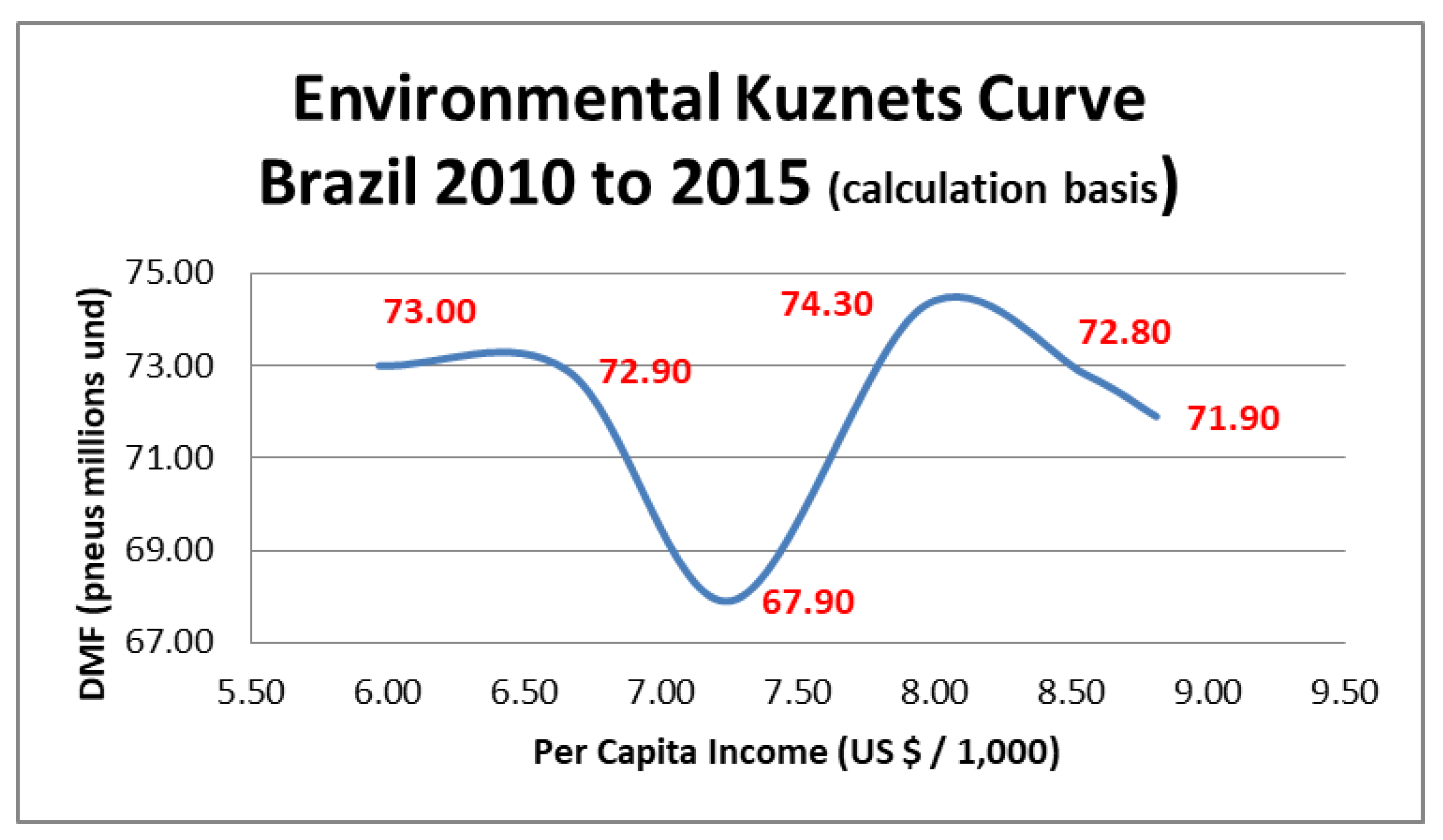
| EKC | Environmental Kuznets Curve |
| PLS | Partial Least Square |
| AVE | Extracted Variance |
| IOA | Input and Output Analysis |
| LCA | Life Cycle Analysis |
| PGIRP | Integrated Pneumatic Waste Management Plan |
| USWM | Urban Solid Waste Management |
| NATI | National Association of Tire Industries |
| EPR | Extended Producer Responsibility |
| CONAMA | National Environmental Council |
2. Literature Review
3. Materials and Methods
3.1. Choice of the PLS Method
3.2. Definition of Variables
3.3. Sampling
- (i)
- Audience profile:
- Definition of the number of indicators.
- (ii)
- Definition of the power of the statistical test and the effect of exogenous variables (f2). [58,81] recommend the use of test power 0.80 and the average effect size (f2) equal to 0.15. Heterogeneous composition with random search of respondents from five segments of society (Civil servant, employee in the private sector, tire and correlated entrepreneurs, university teaching staff and students). Most factory direct employees and manufacturing specialists, including RL professionals, were not selected to avoid bias in technical issues (indicators).
3.4. Measurement and Structural Analysis
- Internal consistency.
- Convergent validity.
- Validity of the discriminant of the measurement model.
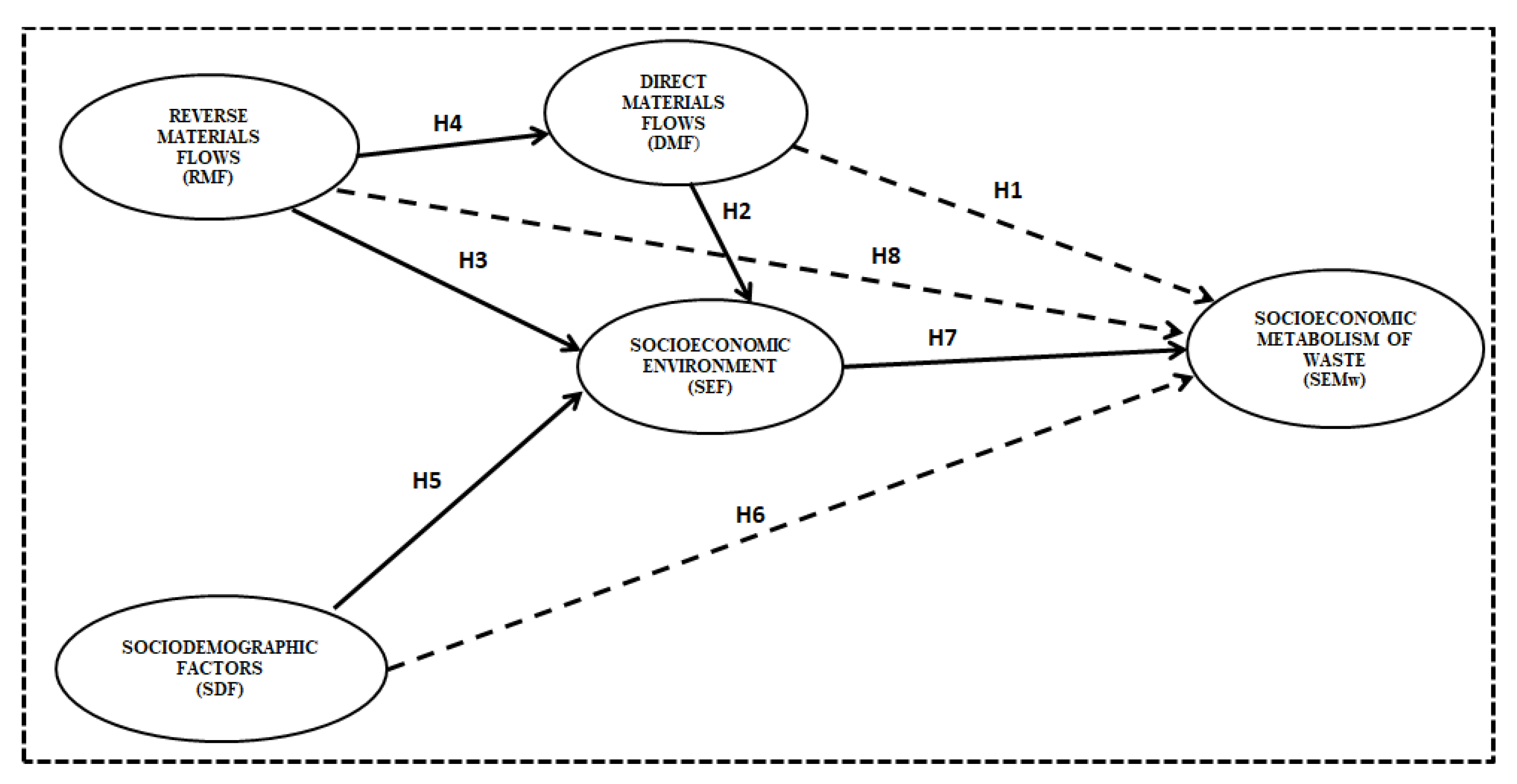
3.5. Modeling Hypothesis
3.6. Justification for the Hypothesis
4. Results and Discussion
4.1. Demographic Profile
4.2. Exploratory Factor Analysis
4.3. Measurement Model Analysis
4.4. Analysis of Hypotheses and Path Coefficients (β)
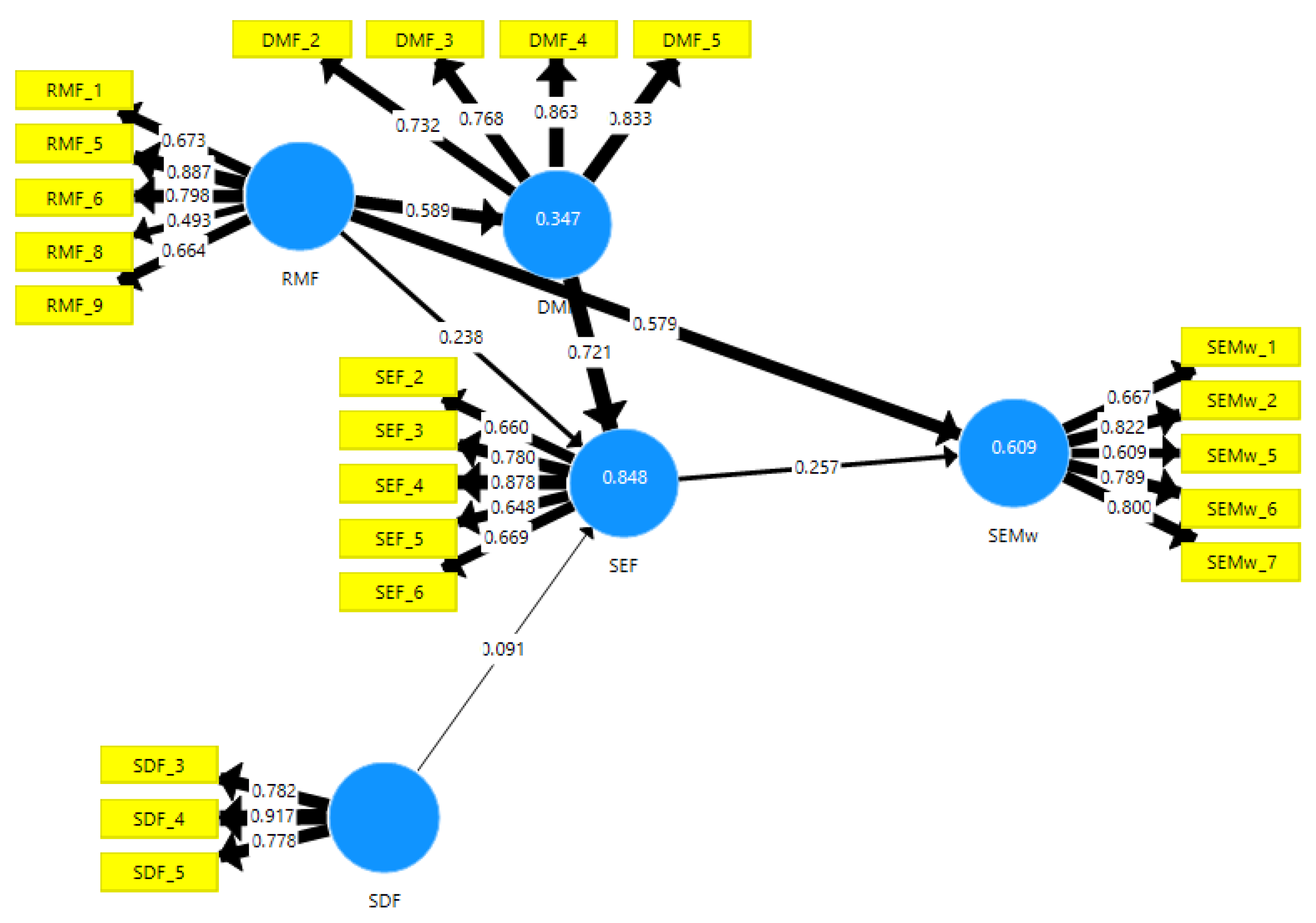
4.5. Analysis of the Structural Model
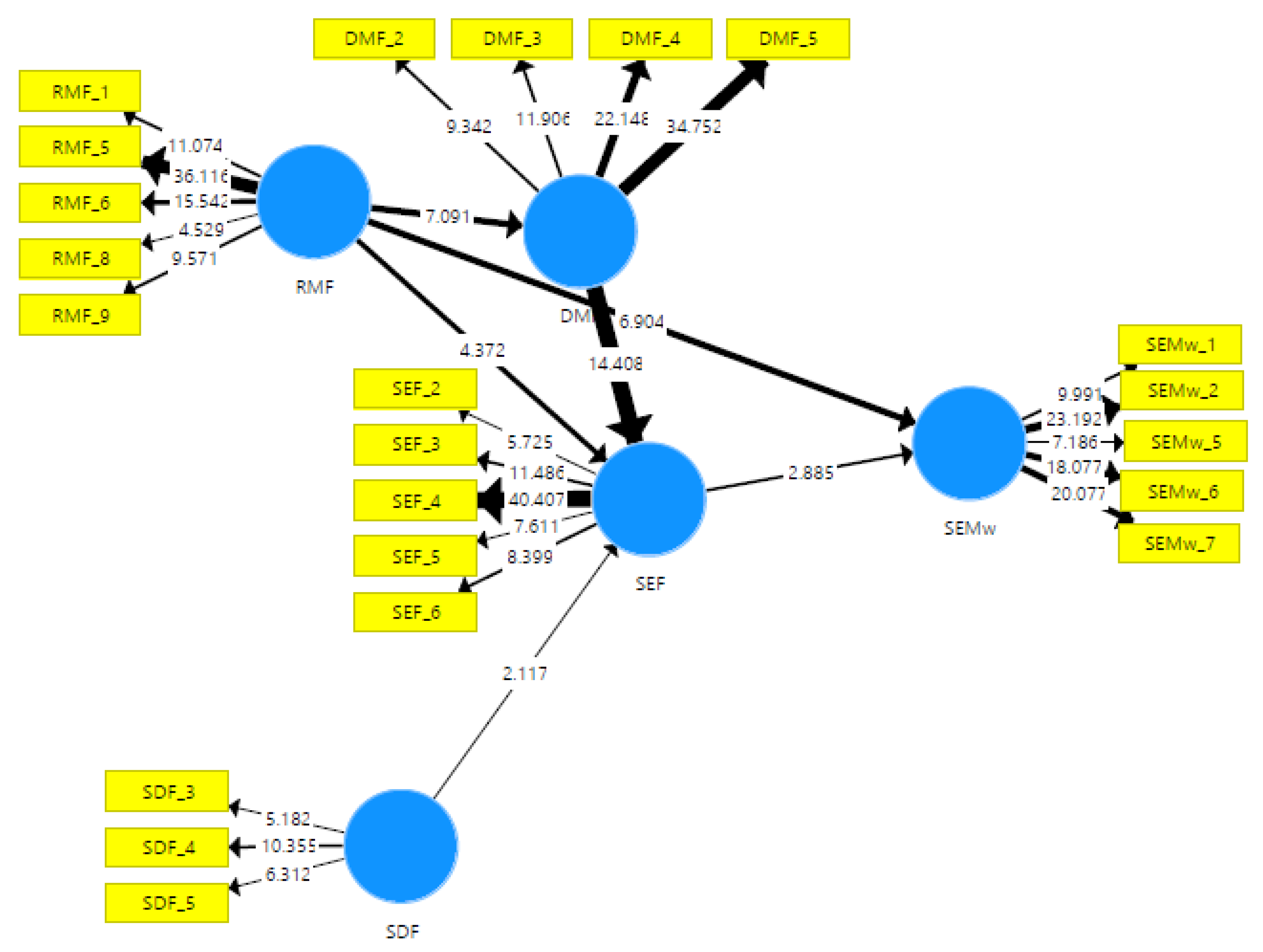
4.6. Analysis of the Structural Model
5. Model Construction as a Tool for Waste Management
6. Conclusions
- (i)
- Theoretical implications of modeling the phenomenon
- (ii)
- Implications for ELT management
7. Recommendations and Future Work
Author Contributions
Funding
Acknowledgments
Conflicts of Interest
Appendix A

| Item | Construct–Socioeconomic Metabolism of Waste (SEMw) |
|---|---|
| What is the importance (…) to evaluate the socioeconomic metabolism of SEMw: (1 = low importance, 5 = high importance) | |
| SEMw_1 | of the ENVIRONMENTAL COST |
| SEMw_2 | of MATERIAL FLOW ANALYSIS (MFA) |
| SEMw_3 | of CIRCULAR ECONOMY conditions |
| SEMw_4 | of the ECONOMIC VALUE of recycled materials |
| SEMw_5 | of LIFE CYCLE analysis (LCA) |
| SEMw_6 | of accounting for MASS BALANCE |
| SEMw_7 | of INPUT AND OUTPUT ANALYSIS (IOA) |
| SEMw_8 | of METABOLIC RATE WASTE MEASUREMENT |
| ITEM | CONSTRUCT—DIRECT MATERIAL FLOWS (DMF) |
| What is the importance (…) in evaluating direct material flows in SEMw? (1 = low importance, 5 = high importance) | |
| DMF_1 | of the wholesaler new tire SUPPLIER NETWORK… |
| DMF_2 | of the retailer SUPPLIER NETWORK for new tires. |
| DMF_3 | of tire DEMAND… |
| DMF_4 | of tire REQUESTS |
| DMF_5 | of the LOCATION OF TIRE SUPPLIERS |
| DMF_6 | of the REGULATION that establishes conditioning factors |
| DMF_7 | of tire MARKETING |
| ITEM | CONSTRUCT—REVERSE MATERIAL FLOWS (DMF) |
| What is the importance (…) to evaluate the reverse material flows in SEMw? (1 = low importance, 5 = high importance) | |
| RMF_1 | ELT COLLECTION in the city |
| RMF_2 | of URBAN PLANNING of the city regarding the collection of ELTs |
| RMF_3 | Accumulation of End-of-Life Tires (ELTs) |
| RMF_4 | EXTERNALITIES (imports) of ELTs |
| RMF_5 | of the final destination of ELTs |
| RMF_6 | of ELTs RECYCLING |
| RMF_7 | of ELTs retreading… |
| RMF_8 | WASTE FLOW PREDICTIONS (ELTS) |
| RMF_9 | of WASTE MANAGEMENT in the city |
| RMF_10 | of the training of the urban cleaning team |
| ITEM | CONSTRUCT—SOCIO-ECONOMIC ENVIRONMENT (SEE) |
| What is the importance (…) in the evaluation of SEMw? (1 = low importance, 5 = high importance) | |
| SEF_1 | of the municipal INVESTMENT |
| SEF _2 | of municipal POLICY in cleaning the city |
| SEF _3 | of BASIC SANITATION in cleaning the city |
| SEF _4 | of GDP (aggregate income) of tire economy |
| SEF _5 | of tire and ELT consumption |
| SEF _6 | of the local CULTURE |
| ITEM | CONSTRUCT—SOCIODEMOGRAPHIC FACTORS (SDF) |
| What is the importance (…) in the evaluation of SEMw? (1 = low importance, 5 = high importance) | |
| SDF_1 | of FAMILY COMPOSITION |
| SDF_2 | of the PROFESSIONAL ACTIVITY of the population |
| SDF_3 | of per capita income of the population. |
| SDF_4 | of the level of education of society |
| SDF_5 | of POPULATIONAL DENSITY. |
| SDF_6 | of the AGE of society |
| SDF_7 | of URBAN SPACE |
References
- Schröder, P.; Vergragt, P.; Brown, H.S.; Dendler, L.; Gorenflo, N.; Matus, K.; Quist, J.; Rupprecht, C.D.; Tukker, A.; Wennersten, R. Advancing sustainable consumption and production in cities-A transdisciplinary research and stakeholder engagement framework to address consumption-based emissions and impacts. J. Clean. Prod. 2019, 213, 114–125. [Google Scholar] [CrossRef]
- Witt, U. The evolution of consumption and its welfare effects. J. Evol. Econ. 2017, 27, 273–293. [Google Scholar] [CrossRef] [PubMed][Green Version]
- Jaiswal, A.; Kumar, S. Waste Legislation Across the Globe: An Overview. In Current Developments in Biotechnology and Bioengineering; Elsevier: Amsterdam, The Netherlands, 2019; pp. 11–30. [Google Scholar]
- Ghinea, C.; Drăgoi, E.N.; Comăniţă, E.D.; Gavrilescu, M.; Câmpean, T.; Curteanu, S.I.L.V.I.A.; Gavrilescu, M. Forecasting municipal solid waste generation using prognostic tools and regression analysis. J. Environ. Manag. 2016, 182, 80–93. [Google Scholar] [CrossRef]
- Kallel, A.; Serbaji, M.M.; Zairi, M. Using GIS-Based tools for the optimization of solid waste collection and transport: Case study of Sfax City, Tunisia. J. Eng. 2016, 2016. [Google Scholar] [CrossRef]
- Srivastava, S.; Jamwal, D.S. Determinants of awareness and disposal habits of households for effective municipal solid waste management. J. Glob. Bus. Adv. 2019, 12, 405–428. [Google Scholar] [CrossRef]
- Zouboulis, A.I.; Peleka, E.N. “Cycle closure” in waste management: Tools, procedures and examples. Glob. Nest J. 2019, 21, 1–6. [Google Scholar]
- Adipah, S. Challenges and Improvement Opportunities for Accra City MSWM System. J. Environ. Sci. 2019, 3, 133–146. [Google Scholar] [CrossRef]
- Cocarta, D.M.; Rada, E.C.; Ragazzi, M.; Badea, A.; Apostol, T. A contribution for a correct vision of health impact from municipal solid waste treatments. Environ. Technol. 2009, 30, 963–968. [Google Scholar] [CrossRef]
- Ferronato, N.; Torretta, V.; Ragazzi, M.; Rada, E.C. Waste mismanagement in developing countries: A case study of environmental contamination. UPB Sci. Bull. 2017, 79, 185–196. [Google Scholar]
- Van Fan, Y.; Klemeš, J.J.; Walmsley, T.G.; Bertók, B. Implementing Circular Economy in municipal solid waste treatment system using P-graph. Sci. Total Environ. 2020, 701, 134652. [Google Scholar] [CrossRef]
- Ziraba, A.K.; Haregu, T.N.; Mberu, B. A review and framework for understanding the potential impact of poor solid waste management on health in developing countries. Arch. Public Health 2016, 74, 55. [Google Scholar] [CrossRef]
- Mohee, R.; Simelane, T. Future Directions of Municipal Solid Waste Management in Africa; Africa Institute of South Africa: Pretoria, South Africa, 2015. [Google Scholar]
- Aderemi, A.O.; Oriaku, A.V.; Adewumi, G.A.; Otitoloju, A.A. Technology. Assessment of groundwater contamination by leachate near a municipal solid waste landfill. J. Environ. Sci. Technol. 2011, 5, 933–940. [Google Scholar]
- Han, Z.; Ma, H.; Shi, G.; He, L.; Wei, L.; Shi, Q. A review of groundwater contamination near municipal solid waste landfill sites in China. Sci. Total Environ. 2016, 569, 1255–1264. [Google Scholar] [CrossRef]
- Chen, G.; Sun, Y.; Xu, Z.; Shan, X.; Chen, Z. Assessment of Shallow Groundwater Contamination Resulting from a Municipal Solid Waste Landfill—A Case Study in Lianyungang, China. Water 2019, 11, 2496. [Google Scholar] [CrossRef]
- Yousefloo, A.; Babazadeh, R. Designing an integrated municipal solid waste management network: A case study. J. Clean. Prod. 2020, 244, 118824. [Google Scholar] [CrossRef]
- Cecchin, A.; Lamour, M.; Joseph Maks Davis, M.; Jácome Polit, D. End-of-life product management as a resilience driver for developing countries: A policy experiment for used tires in Ecuador. J. Ind. Ecol. 2019, 23, 1292–1310. [Google Scholar] [CrossRef]
- Ishola Felix, A.; Ajayi Oluseyi, O.; Oyawale, F.; Akinlabi, S.A. Sustainable End-of-Life Tyre (EOLT) Management for Developing Countries–A Review. In Proceedings of the International Conference on Industrial Engineering and Operations Management, Pretoria/Johannesburg, South Africa, 29 October–1 November 2018. [Google Scholar]
- Torretta, V.; Rada, E.C.; Ragazzi, M.; Trulli, E.; Istrate, I.A.; Cioca, L.I. Treatment and disposal of tyres: Two EU approaches. A review. Waste Manag. 2015, 45, 152–160. [Google Scholar] [CrossRef]
- Rada, E.C.; Ragazzi, M.; Dal Maschio, R.; Ischia, M.; Panaitescu, V.N. Politehnica University of Bucharest, Series D, Mechanical Engineering. Energy recovery from tyres waste through thermal option. Sci. Bull. Politeh. Univ. Buchar. Ser. D Mech. Eng. 2012, 74, 201–210. [Google Scholar]
- Stanojević, D.D.; Rajković, M.B.; Tošković, D.V. Management of used tires, accomplishments in the world, and situation in Serbia. Hemijska Industrija 2011, 65, 727–738. [Google Scholar] [CrossRef]
- Sienkiewicz, M.; Kucinska-Lipka, J.; Janik, H.; Balas, A. Progress in used tyres management in the European Union: A review. Waste Manag. 2012, 32, 1742–1751. [Google Scholar] [CrossRef]
- Aliabdo, A.A.; Abd Elmoaty, A.E.M.; AbdElbaset, M.M. Utilization of waste rubber in non-structural applications. Constr. Build. Mater. 2015, 91, 195–207. [Google Scholar] [CrossRef]
- Ribeiro Filho, S.L.M.; Oliveira, P.R.; Panzera, T.H.; Scarpa, F. Impact of hybrid composites based on rubber tyres particles and sugarcane bagasse fibres. Compos. Part B Eng. 2019, 159, 157–164. [Google Scholar] [CrossRef]
- Perondi, D.; Marcolin, P.; Biondo, L.; de Souza, G.; de Matos, E.F.; Dettmer, A.; Godinho, M.; Vilela, A.C.F. Co-Pirólise De Resíduos De Pneus E Resina Polimérica Presente Na Areia De Fundição. In Proceedings of the 8th International Bioenergy Congress, Sao Paulo, Brazil, 5–7 November 2013. [Google Scholar]
- Marchiori, H. Estudo de Viabilidade da Aplicação de Pneus Como Combustível na Geração de Energia Elétrica. Available online: http://sites.poli.usp.br/d/pme2600/2007/Artigos/Art_TCC_059_2007.pdf (accessed on 12 January 2020).
- Mmereki, D.; Machola, B.; Mokokwe, K. Status of waste tires and management practice in Botswana. J. Air Waste Manag. Assoc. 2019, 69, 1230–1246. [Google Scholar] [CrossRef]
- Fischer-Kowalski, M. Regional and National Material Flow Accounting: From Paradigm to Practice of Sustainability; Science Centre North Rhine-Westphalia: Wuppertal, Germany, 1997. [Google Scholar]
- Hertz, T.; Schlüter, M. The SES-framework as boundary object to address theory orientation in social–ecological system research: The SES-TheOr approach. Ecol. Econ. 2015, 116, 12–24. [Google Scholar] [CrossRef]
- Cammack, R.; Atwood, T.; Campbell, P.; Parish, H.; Smith, A.; Vella, F.; Stirling, J. Metabolism; Oxford Dictionary of Biochemistry and Molecular Biology; Oxford University Press: Oxford, UK, 2008. [Google Scholar]
- Ayres, R.U.; Simonis, U.E. Industrial Metabolism: Restructuring for Sustainable Development; United Nations University Press: New York, NY, USA, 1994. [Google Scholar]
- Baccini, P.; Brunner, P.H. Metabolism of the Anthroposphere; Springer: Berlin/Heidelberg, Germany, 1991. [Google Scholar]
- Baccini, P.; Brunner, P.H. Metabolism of the Anthroposphere: Analysis, Evaluation, Design; MIT Press: Cambridge, MA, USA, 2012. [Google Scholar]
- Fischer-Kowalski, M. Society’s metabolism: The intellectual history of materials flow analysis, Part I, 1860–1970. J. Ind. Ecol. 1998, 2, 61–78. [Google Scholar] [CrossRef]
- Wolman, A. The metabolism of cities. Sci. Am. 1965, 213, 178–193. [Google Scholar] [CrossRef]
- Pauliuk, S.; Hertwich, E.G. Prospective models of society’s future metabolism: What industrial ecology has to contribute. In Taking Stock of Industrial Ecology; Springer: Cham, Germany, 2016; pp. 21–43. [Google Scholar]
- Allesch, A.; Brunner, P.H. Material flow analysis as a decision support tool for waste management: A literature review. J. Ind. Ecol. 2015, 19, 753–764. [Google Scholar] [CrossRef]
- Pauliuk, S.; Majeau-Bettez, G.; Müller, D.B. A general system structure and accounting framework for socioeconomic metabolism. J. Ind. Ecol. 2015, 19, 728–741. [Google Scholar] [CrossRef]
- Fischer-Kowalski, M.; Haberl, H. El metabolismo socieconómico. Ecología Política 2000, 19, 21–33. [Google Scholar]
- Pauliuk, S.; Müller, D.B. The role of in-use stocks in the social metabolism and in climate change mitigation. Glob. Environ. Chang. 2014, 24, 132–142. [Google Scholar] [CrossRef]
- Fischer-Kowalski, M.; Haberl, H. Socioecological Transitions and Global Change: Trajectories of Social Metabolism and Land Use; Edward Elgar: Cheltenham, UK; Northampton, MA, USA, 2007. [Google Scholar]
- Fischer-Kowalski, M.; Weisz, H. Society as hybrid between material and symbolic realms: Toward a theoretical framework of society-nature interaction. Adv. Hum. Ecol. 1999, 8, 215–252. [Google Scholar]
- Kennedy, C.; Cuddihy, J.; Engel-Yan, J. The changing metabolism of cities. J. Ind. Ecol. 2007, 11, 43–59. [Google Scholar] [CrossRef]
- Newell, J.P.; Cousins, J.J. The boundaries of urban metabolism: Towards a political-industrial ecology. Prog. Hum. Geogr. 2015, 39, 702–728. [Google Scholar] [CrossRef]
- Wang, Y.; Chen, P.-C.; Ma, H.-W.; Cheng, K.-L.; Chang, C.-Y. Socio-economic metabolism of urban construction materials: A case study of the Taipei metropolitan area. Resour. Conserv. Recycl. 2018, 128, 563–571. [Google Scholar] [CrossRef]
- Li, H.; Kwan, M.-P. Advancing analytical methods for urban metabolism studies. Resour. Conserv. Recycl. 2018, 132, 239–245. [Google Scholar] [CrossRef]
- Zhang, Y.; Yang, Z.; Yu, X. Urban metabolism: A review of current knowledge and directions for future study. Environ. Sci. Technol. 2015, 49, 11247–11263. [Google Scholar] [CrossRef]
- Dai, T.; Wang, W. The characteristics and trends of socioeconomic metabolism in China. J. Ind. Ecol. 2018, 22, 1228–1240. [Google Scholar] [CrossRef]
- Fami, H.S.; Aramyan, L.H.; Sijtsema, S.J.; Alambaigi, A. Determinants of household food waste behavior in Tehran city: A structural model. Resour. Conserv. Recycl. 2019, 143, 154–166. [Google Scholar] [CrossRef]
- Srun, P.; Kurisu, K. Internal and External Influential Factors on Waste Disposal Behavior in Public Open Spaces in Phnom Penh, Cambodia. Sustainability 2019, 11, 1518. [Google Scholar] [CrossRef]
- Ma, B.; Li, X.; Jiang, Z.; Jiang, J. Recycle more, waste more? When recycling efforts increase resource consumption. J. Clean. Prod. 2019, 206, 870–877. [Google Scholar] [CrossRef]
- Arı, E.; Yılmaz, V. A proposed structural model for housewives’ recycling behavior: A case study from Turkey. Ecol. Econ. 2016, 129, 132–142. [Google Scholar] [CrossRef]
- Lu, M.; Wei, M. Analysis of the Factors Affected Construction Waste’s Management in Structure Equation Model. Advanced Materials Research. Adv. Mater. Res. Trans. Tech. Publ. Ltd 2014, 878, 315–321. [Google Scholar] [CrossRef]
- Kannan, D.; Diabat, A.; Shankar, K.M. Analyzing the drivers of end-of-life tire management using interpretive structural modeling (ISM). Int. J. Adv. Manuf. Technol. 2014, 72, 1603–1614. [Google Scholar] [CrossRef]
- Beigl, P.; Lebersorger, S.; Salhofer, S. Modelling municipal solid waste generation: A review. Waste Manag. 2008, 28, 200–214. [Google Scholar] [CrossRef] [PubMed]
- Durdyev, S.; Ihtiyar, A.; Banaitis, A.; Thurnell, D. The construction client satisfaction model: A PLS-SEM approach. J. Civil. Eng. Manag. 2018, 24, 31–42. [Google Scholar] [CrossRef]
- Hair, J.F., Jr.; Sarstedt, M.; Ringle, C.M.; Gudergan, S.P. Advanced Issues in Partial Least Squares Structural Equation Modeling; SAGE Publications: Newcastle upon Tyne, UK, 2017. [Google Scholar]
- Reinartz, W.; Haenlein, M.; Henseler, J. An empirical comparison of the efficacy of covariance-based and variance-based SEM. Int. J. Res. Mark. 2009, 26, 332–344. [Google Scholar] [CrossRef]
- Sarstedt, M.; Hair, J.F.; Ringle, C.M.; Thiele, K.O.; Gudergan, S.P. Estimation issues with PLS and CBSEM: Where the bias lies! J. Bus. Res. 2016, 69, 3998–4010. [Google Scholar] [CrossRef]
- Rigdon, E.E.; Sarstedt, M.; Ringle, C.M. On comparing results from CB-SEM and PLS-SEM: Five perspectives and five recommendations. Mark. Zfp 2017, 39, 4–16. [Google Scholar] [CrossRef]
- Streukens, S.; Leroi-Werelds, S. Bootstrapping and PLS-SEM: A step-by-step guide to get more out of your bootstrap results. Eur. Manag. J. 2016, 34, 618–632. [Google Scholar] [CrossRef]
- Henseler, J.; Ringle, C.M.; Sinkovics, R.R. The use of partial least squares path modeling in international marketing. In New Challenges to International Marketing; Emerald Group Publishing Limited: England, UK, 2009; pp. 277–319. [Google Scholar]
- Davari, A.; Rezazadeh, A. Structural equation modeling with PLS. Tehran Jahad Univ. 2013, 215, 224. [Google Scholar]
- Krausmann, F.; Gingrich, S.; Nourbakhch-Sabet, R. The metabolic transition in Japan: A material flow account for the period from 1878 to 2005. J. Ind. Ecol. 2011, 15, 877–892. [Google Scholar] [CrossRef]
- Fischer-Kowalski, M.; Krausmann, F.; Giljum, S.; Lutter, S.; Mayer, A.; Bringezu, S.; Moriguchi, Y.; Schütz, H.; Schandl, H.; Weisz, H. Methodology and indicators of economy-wide material flow accounting. J. Ind. Ecol. 2011, 15, 855–876. [Google Scholar] [CrossRef]
- Fischer-Kowalski, M.; Krausmann, F.; Pallua, I. A sociometabolic reading of the Anthropocene: Modes of subsistence, population size and human impact on Earth. Anthr. Rev. 2014, 1, 8–33. [Google Scholar] [CrossRef]
- Krausmann, F.; Lauk, C.; Haas, W.; Wiedenhofer, D. From resource extraction to outflows of wastes and emissions: The socioeconomic metabolism of the global economy, 1900–2015. Glob. Environ. Chang. 2018, 52, 131–140. [Google Scholar] [CrossRef]
- CONAMA. Resolução 416 de 30 de Setembro de 2009. Available online: http://www2.mma.gov.br/port/conama/legiabre.cfm?codlegi=616 (accessed on 12 January 2020).
- Shulman, V.L. Tire Recycling; Smithers Rapra Press: Shropshire, UK, 1999. [Google Scholar]
- Gupt, Y.; Sahay, S. Review of extended producer responsibility: A case study approach. Waste Manag. Res. 2015, 33, 595–611. [Google Scholar] [CrossRef]
- Fagundes, L.D.; Amorim, E.S.; da Silva Lima, R. Action research in reverse logistics for end-of-life tire recycling. Syst. Pract. Action Res. 2017, 30, 553–568. [Google Scholar] [CrossRef]
- Schultmann, F.; Zumkeller, M.; Rentz, O. Modeling reverse logistic tasks within closed-loop supply chains: An example from the automotive industry. Eur. J. Oper. Res. 2006, 171, 1033–1050. [Google Scholar] [CrossRef]
- Govindan, K.; Soleimani, H.; Kannan, D. Reverse logistics and closed-loop supply chain: A comprehensive review to explore the future. Eur. J. Oper. Res. 2015, 240, 603–626. [Google Scholar] [CrossRef]
- Agrawal, S.; Singh, R.K.; Murtaza, Q. A literature review and perspectives in reverse logistics. Resour. Conserv. Recycl. 2015, 97, 76–92. [Google Scholar] [CrossRef]
- Adzawla, W.; Tahidu, A.; Mustapha, S.; Azumah, S.B. Do socioeconomic factors influence households’ solid waste disposal systems? Evidence from Ghana. Waste Manag. Res. 2019, 37, 51–57. [Google Scholar] [CrossRef]
- Rybova, K. Do Sociodemographic Characteristics in Waste Management Matter? Case Study of Recyclable Generation in the Czech Republic. Sustainability 2019, 11, 2030. [Google Scholar] [CrossRef]
- Hair, J.F., Jr.; Sarstedt, M.; Hopkins, L.; Kuppelwieser, V.G. Partial least squares structural equation modeling (PLS-SEM) An emerging tool in business research. Eur. Bus. Rev. 2014, 26, 106–121. [Google Scholar] [CrossRef]
- Lu, J.-W.; Chang, N.-B.; Zhu, F.; Hai, J.; Liao, L. Smart and green urban solid waste collection system for differentiated collection with integrated sensor networks. In Proceedings of the Networking, Sensing and Control (ICNSC), 2018 IEEE 15th International Conference on, Zhuhai, China, 27–29 March 2018; pp. 1–5. [Google Scholar]
- Wisner, J.D. A structural equation model of supply chain management strategies and firm performance. J. Bus. Logist. 2003, 24, 1–26. [Google Scholar] [CrossRef]
- Cohen, J. Statistical Power Analysis for the Behavioral Sciences; Routledge: Abingdon, UK, 2013. [Google Scholar]
- Hair, J.F.; Ringle, C.M.; Gudergan, S.P.; Fischer, A.; Nitzl, C.; Menictas, C. Partial least squares structural equation modeling-based discrete choice modeling: An illustration in modeling retailer choice. Bus. Res. 2019, 12, 115–142. [Google Scholar] [CrossRef]
- Davison, A.C.; Hinkley, D.V. Bootstrap Methods and Their Application; Cambridge University press: Cambridge, UK, 1997. [Google Scholar]
- Wong, K.K.-K. Mastering Partial Least Squares Structural Equation Modeling (PLS-SEM) with Smartpls in 38 Hours; iUniverse: Bloomington, IN, USA, 2019. [Google Scholar]
- Hair, J.F., Jr.; Hult, G.T.M.; Ringle, C.; Sarstedt, M. A Primer on Partial Least Squares Structural Equation Modeling (PLS-SEM); Sage publications: New York, NY, USA, 2016. [Google Scholar]
- Chin, W.W. The partial least squares approach to structural equation modeling. Mod. Methods Bus. Res. 1998, 295, 295–336. [Google Scholar]
- Fornell, C.; Larcker, D.F. Structural Equation Models with Unobservable Variables and Measurement Error: Algebra and Statistics; SAGE Publications Sage CA: Los Angeles, CA, USA, 1981. [Google Scholar]
- Hair, J.F.; Risher, J.J.; Sarstedt, M.; Ringle, C.M. When to use and how to report the results of PLS-SEM. Eur. Bus. Rev. 2019, 31, 2–24. [Google Scholar] [CrossRef]
- Dijkstra, T.K.; Henseler, J. Consistent partial least squares path modeling. MIS Q. 2015, 39, 297–316. [Google Scholar] [CrossRef]
- Sarstedt, M.; Ringle, C.M.; Henseler, J.; Hair, J.F. On the emancipation of PLS-SEM: A commentary on Rigdon (2012). Long Range Plan. 2014, 47, 154–160. [Google Scholar] [CrossRef]
- Cohen, J. Statistical Power Analysis for the Behaviors Science, 2nd ed.; Laurence Erlbaum Associates: Hillsdale, MN, USA, 1988. [Google Scholar]
- Pedram, A.; Yusoff, N.B.; Udoncy, O.E.; Mahat, A.B.; Pedram, P.; Babalola, A. Integrated forward and reverse supply chain: A tire case study. Waste Manag. 2017, 60, 460–470. [Google Scholar] [CrossRef]
- Antoniou, N.; Zabaniotou, A. Re-designing a viable ELTs depolymerization in circular economy: Pyrolysis prototype demonstration at TRL 7, with energy optimization and carbonaceous materials production. J. Clean. Prod. 2018, 174, 74–86. [Google Scholar] [CrossRef]
- Maderuelo-Sanz, R.; Nadal-Gisbert, A.V.; Crespo-Amorós, J.E.; Parres-García, F. A novel sound absorber with recycled fibers coming from end of life tires (ELTs). Appl. Acoust. 2012, 73, 402–408. [Google Scholar] [CrossRef]
- Pehlken, A.; Müller, D.H. Using information of the separation process of recycling scrap tires for process modelling. Resour. Conserv. Recycl. 2009, 54, 140–148. [Google Scholar] [CrossRef]
- Haberl, H.; Steinberger, J.K.; Plutzar, C.; Erb, K.H.; Gaube, V.; Gingrich, S.; Krausmann, F. Natural and socioeconomic determinants of the embodied human appropriation of net primary production and its relation to other resource use indicators. Ecol. Indic. 2012, 23, 222–231. [Google Scholar] [CrossRef] [PubMed]
- Shah, K.U.; Niles, K.; Ali, S.H.; Surroop, D.; Jaggeshar, D. Plastics Waste Metabolism in a Petro-Island State: Towards Solving a “Wicked Problem” in Trinidad and Tobago. Sustainability 2019, 11, 6580. [Google Scholar] [CrossRef]
- Marega, F. The Retreaded Tyres Case in WTO: An Important Multilateral Achievement by Brazil. In The WTO Dispute Settlement Mechanism; Springer: Berlin/Heidelberg, Germany, 2019; pp. 321–338. [Google Scholar]
- IBGE. Tire sales in Brazil from 2010 to 2015. In Diretoria de Pesquisas, Coordenação de Contas Nacionais; Instituto Brasileiro de Geografia e Estatística: Rio de Janeiro, Brazil, 2020. [Google Scholar]
- Mazzanti, M.; Montini, A.; Zoboli, R. Municipal waste generation and socioeconomic drivers: Evidence from comparing Northern and Southern Italy. J. Environ. Dev. 2008, 17, 51–69. [Google Scholar] [CrossRef]
- Lonca, G.; Muggéo, R.; Imbeault-Tétreault, H.; Bernard, S.; Margni, M. Does material circularity rhyme with environmental efficiency? Case studies on used tires. J. Clean. Prod. 2018, 183, 424–435. [Google Scholar] [CrossRef]
- Megiddo, T. Beyond Fragmentation: On International Law’s Integrationist Forces. Yale J. Int. Law 2019, 44, 4. [Google Scholar]
- Krausmann, F.; Wiedenhofer, D.; Lauk, C.; Haas, W.; Tanikawa, H.; Fishman, T.; Miatto, A.; Schandl, H.; Haberl, H. Global socioeconomic material stocks rise 23-fold over the 20th century and require half of annual resource use. Proc. Natl. Acad. Sci. USA 2017, 114, 1880–1885. [Google Scholar] [CrossRef]
- Pauliuk, S.; Wood, R.; Hertwich, E.G. Dynamic models of fixed capital stocks and their application in industrial ecology. J. Ind. Ecol. 2015, 19, 104–116. [Google Scholar] [CrossRef]
- Fishman, T.; Schandl, H.; Tanikawa, H. The socio-economic drivers of material stock accumulation in Japan’s prefectures. Ecol. Econ. 2015, 113, 76–84. [Google Scholar] [CrossRef]
- Mazzanti, M.; Zoboli, R. Waste generation, waste disposal and policy effectiveness: Evidence on decoupling from the European Union. Resour. Conserv. Recycl. 2008, 52, 1221–1234. [Google Scholar] [CrossRef]
- Dombi, M.; Karcagi-Kováts, A.; Tóth-Szita, K.; Kuti, I. The structure of socio-economic metabolism and its drivers on household level in Hungary. J. Clean. Prod. 2018, 172, 758–767. [Google Scholar] [CrossRef]
- Strobel, M.; Redmann, C. Flow cost accounting, an accounting approach based on the actual flows of materials. In Environmental Management Accounting: Informational and Institutional Developments; Springer: Berlin/Heidelberg, Germany, 2002; pp. 67–82. [Google Scholar]
- Cole, M.A.; Rayner, A.J.; Bates, J.M. The environmental Kuznets curve: An empirical analysis. Environ. Dev. Econ. 1997, 2, 401–416. [Google Scholar] [CrossRef]
- Chang, N.-B. Economic and policy instrument analyses in support of the scrap tire recycling program in Taiwan. J. Environ. Manag. 2008, 86, 435–450. [Google Scholar] [CrossRef] [PubMed]
- Ferrer, G. The economics of tire remanufacturing. Resour. Conserv. Recycl. 1997, 19, 221–255. [Google Scholar] [CrossRef]
- Govindan, K.; Palaniappan, M.; Zhu, Q.; Kannan, D. Analysis of third party reverse logistics provider using interpretive structural modeling. Int. J. Prod. Econ. 2012, 140, 204–211. [Google Scholar] [CrossRef]
- Ramayah, T.; Lee, J.W.C.; Lim, S. Sustaining the environment through recycling: An empirical study. J. Environ. Manag. 2012, 102, 141–147. [Google Scholar] [CrossRef]
- Barr, S. Household Waste in Social Perspective: Values, Attitudes, Situation and Behaviour; Routledge: Abingdon, UK, 2017. [Google Scholar]
- Haas, W.; Krausmann, F.; Wiedenhofer, D.; Heinz, M. How circular is the global economy?: An assessment of material flows, waste production, and recycling in the European Union and the world in 2005. J. Ind. Ecol. 2015, 19, 765–777. [Google Scholar] [CrossRef]
- Swami, V.; Chamorro-Premuzic, T.; Snelgar, R.; Furnham, A. Personality, individual differences, and demographic antecedents of self-reported household waste management behaviours. J. Environ. Psychol. 2011, 31, 21–26. [Google Scholar] [CrossRef]
- Chang, N.-B.; Pires, A.; Martinho, G. Empowering systems analysis for solid waste management: Challenges, trends, and perspectives. Crit. Rev. Environ. Sci. Technol. 2011, 41, 1449–1530. [Google Scholar] [CrossRef]
- Rybova, K.; Burcin, B.; Slavik, J. Spatial and non-spatial analysis of socio-demographic aspects influencing municipal solid waste generation in the Czech Republic. Detritus 2018, 1, 3. [Google Scholar]
- Xu, L.; Lin, T.; Xu, Y.; Xiao, L.; Ye, Z.; Cui, S. Path analysis of factors influencing household solid waste generation: A case study of Xiamen Island, China. J. Mater. Cycles Waste Manag. 2016, 18, 377–384. [Google Scholar] [CrossRef]
- Kannangara, M.; Dua, R.; Ahmadi, L.; Bensebaa, F. Modeling and prediction of regional municipal solid waste generation and diversion in Canada using machine learning approaches. Waste Manag. 2018, 74, 3–15. [Google Scholar] [CrossRef]
- Bach, H.; Mild, A.; Natter, M.; Weber, A. Combining socio-demographic and logistic factors to explain the generation and collection of waste paper. Resour. Conserv. Recycl. 2004, 41, 65–73. [Google Scholar] [CrossRef]
- Azevedo, L.P.; Araújo, F.G.D.S.; Lagarinhos, C.A.F.; Tenório, J.A.S.; Espinosa, D.C. Resource Recovery From E-waste for Environmental Sustainability: A Case Study in Brazil. In Electronic Waste Management and Treatment Technology; Elsevier: Amsterdam, The Netherlands, 2019; pp. 175–200. [Google Scholar]
- Madden, B.; Florin, N.; Mohr, S.; Giurco, D. Using the waste Kuznet’s curve to explore regional variation in the decoupling of waste generation and socioeconomic indicators. Resour. Conserv. Recycl. 2019, 149, 674–686. [Google Scholar] [CrossRef]
- Riediger, N.D.; Shooshtari, S.; Moghadasian, M.H. The influence of sociodemographic factors on patterns of fruit and vegetable consumption in Canadian adolescents. J. Am. Diet. Assoc. 2007, 107, 1511–1518. [Google Scholar] [CrossRef]
- Binder, C.R. From material flow analysis to material flow management Part I: Social sciences modeling approaches coupled to MFA. J. Clean. Prod. 2007, 15, 1596–1604. [Google Scholar] [CrossRef]
- Gomes, T.S.; Neto, G.R.; de Salles, A.C.N.; Visconte, L.L.Y.; Pacheco, E.B.A.V. End-of-Life Tire Destination from a Life Cycle Assessment Perspective. In New Frontiers on Life Cycle Assessment-Theory and Application; IntechOpen: London, UK, 2019. [Google Scholar]
- Knickmeyer, D. Social factors influencing household waste separation: A literature review on good practices to improve the recycling performance of urban areas. J. Clean. Prod. 2019, 245, 118605. [Google Scholar] [CrossRef]
- Villela, G.O.M.; Silva, F.B. A logística reversa de pneus. Rev. Vianna Sapiens 2019, 10, 17. [Google Scholar] [CrossRef]
- Hayduk, L.A.; Littvay, L. Should researchers use single indicators, best indicators, or multiple indicators in structural equation models? BMC Med Res. Methodol. 2012, 12, 159. [Google Scholar] [CrossRef]
- Hulland, J. Use of partial least squares (PLS) in strategic management research: A review of four recent studies. Strateg. Manag. J. 1999, 20, 195–204. [Google Scholar] [CrossRef]
- Gefen, D.; Straub, D.; Boudreau, M.-C. Structural equation modeling and regression: Guidelines for research practice. Commun. Assoc. Inf. Syst. 2000, 4, 7. [Google Scholar] [CrossRef]


| Construct | Indicator | Description | Metric (M)/ Non-Metric (N/M) | References |
|---|---|---|---|---|
| Direct Material Flows DMF | DMF_1 | Supplier Network (t) | M | [28,69,70,71] |
| DMF_2 | Supply Network (t) | M | ||
| DMF_3 | Demand (t) | M | ||
| DMF_4 | Requests (t) | M | ||
| DMF_5 | Location | N/M | ||
| DMF_6 | Regulation | N/M | ||
| DMF_7 | Marketing | N/M | ||
| Reverse Material Flows RMF | RMF_1 | Collect (t) | M | [13,23,69,71,72,73,74,75] |
| RMF_2 | Urban planning | N/M | ||
| RMF_3 | Accumulation (t) | M | ||
| RMF_4 | Externalities (t) | M | ||
| RMF_5 | Final Destination (t) | M | ||
| RMF_6 | Recycling (t) | M | ||
| RMF_7 | Retreading (t) | M | ||
| RMF_8 | Forecasts (t) | M | ||
| RMF_9 | Waste Management ($) | M | ||
| RMF_10 | Team training ($) | M | ||
| Sociodemographic Factors SDF | SDF_1 | Family Composition | N/M | [76,77] |
| SDF_2 | Professional Activity ($) | M | ||
| SDF_3 | Per capita income ($/inhabitants) | M | ||
| SDF_4 | Schooling ($/students) | M | ||
| SDF_5 | Population density (Inhabitants/Km2) | M | ||
| SDF_6 | Age (years) | M | ||
| SDF_7 | Urban Space (Km2) | M | ||
| Socioeconomic Environment SEF | SEF_1 | Investment ($) | M | [76,77] |
| SEF_2 | Municipal Policy | N/M | ||
| SEF_3 | Basic Sanitation | N/M | ||
| SEF_4 | GDP (aggregate income) ($) | M | ||
| SEF_5 | Consumption ($) | M | ||
| SEF_6 | Local Culture | N/M | ||
| Socioeconomic Metabolism of Waste SEMw | SEMw_1 | Environmental Cost ($) | M | [30,39,65,66,67,68] |
| SEMw_2 | MFA (t) | M | ||
| SEMw_3 | CE | N/M | ||
| SEMw_4 | Economic value ($) | M | ||
| SEMw_5 | LCA (t) | M | ||
| SEMw_6 | Mass Balance (t) | M | ||
| SEMw_7 | IOA (t) | M | ||
| SEMw_8 | Metabolic Rate (t/years) | M |
| Objective | Measurement | Criteria | References |
|---|---|---|---|
| Indicator | Factorial Load | > 0.708 * | [85] |
| Internal Consistency | Cronbach’s Alpha Composite Reliability rho_A | AC > 0.7 ** CR > 0.7 rho_A > 0.7 *** | |
| Convergent validity | Average variance extracted (AVE) | AVE > 0.5 | |
| Discriminant validity | Cross Loads Fornell and Larcker Criteria | Factorial Load (AVE)2 | [86,87] |
| Objective | Measurement Parameter | Criteria | References |
|---|---|---|---|
| Evaluate the variance of endogenous constructs explained by all exogenous constructs | Pearson’s coefficient of determination (R2) | Between 0 and 1* | [91] |
| Evaluate the effect of the exogenous construct when it is excluded from the model | Effect Size or Cohen Indicator (f2) | 0.02—small effect 0.15—average effect 0.35—big effect | |
| Evaluate the predictive power of originally observed values | Predictive Validity or Stone-Geisser Indicator or Cross-Validity Redundancy (Q2) | 0.02—small relevance 0.15—average relevance 0.35—great relevance | [85] |
| Assess causal relationships | Path coefficient | The ideal tvalue value must be above 1.96 and the path coefficient must be non-zero at a significance level of 5%. |
| Hypothesis | Description | References |
|---|---|---|
| H1 | DMF have a direct effect on SEMw. | [97,98,100,101,102] |
| H2 | DMF have a direct effect on SEF. | [39,55,74,100,103,105,107,108,109,110,111] |
| H3 | RMF have a direct effect SEF. | [49,74,75,107,112,113,114] |
| H4 | H4—RMF have a direct effect on DMF. | [73,74,92,115] |
| H5 | SDF have a direct effect on SEF. | [56,76,77,100,116,117,118,119,120] |
| H6 | SDF have a direct effect on SEMw. | [100,121,122,123,127] |
| H7 | SEF have a direct effect on SEMw. | [76,96,107,124,125] |
| H8 | RMF have a direct effect on SEMw. | [50,75,101,113,126,128] |
| Demographic Characteristics of City (Case Study) Respondents | |||||
|---|---|---|---|---|---|
| Demography | Frequency | % | Demography | Frequency | % |
| Age (years) | Professional Activity | ||||
| <24 | 11 | 11.11 | Civil servant | 25 | 25.25 |
| 25 to 34 | 32 | 32.32 | Private Employee | 26 | 26.26 |
| 35 to 44 | 40 | 40.40 | Businessman | 7 | 7.07 |
| 45 to 54 | 12 | 12.12 | College professor | 20 | 20.20 |
| >55 | 4 | 4.04 | Student | 21 | 21.21 |
| Sex | Education Level | ||||
| Male | 51 | 51.52 | Elementary School | 11 | 11.11 |
| Female | 43 | 43.43 | High school | 31 | 31.31 |
| Other | 5 | 5.05 | University student | 30 | 30.30 |
| Graduate | 27 | 27.27 | |||
| Income | |||||
| <2.5 Minimum Wage (MW) | 16 | 16.16 | |||
| 2.5 MW to 10.5 MW | 23 | 23.23 | |||
| 10.5 MW to 25.5 MW | 40 | 40.40 | |||
| 25.5 MW to 50.5 MW | 17 | 17.17 | |||
| 50.5 MW to 105.5 MW | 3 | 3.03 | |||
| 105.5 MW to 505.5 MW | - | - | |||
| >505.5 MW | - | - | |||
| Construct | Indicator | Description | Factorial Load |
|---|---|---|---|
| Direct Material Flows (DMF) | DMF_1 | Supplier Network | 0.133 |
| DMF_6 | Regulation | 0.430 | |
| DMF_7 | Marketing | 0.451 | |
| Reverse Material Flows (RMF) | RMF_2 | Urban planning | 0.173 |
| RMF_3 | Accumulation | 0.209 | |
| RMF_4 | Externalities | 0.528 | |
| RMF_7 | Retreading | 0.077 | |
| RMF_10 | Team training | 0.045 | |
| Sociodemographic Factors (SDF) | SDF_1 | Family Composition | 0.068 |
| SDF_2 | Professional Activity | 0.194 | |
| SDF_6 | Age | 0.206 | |
| SDF_7 | Urban Space | 0.121 | |
| Socioeconomic Environment (SEF) | SEF_1 | Investment | 0.637 |
| Socioeconomic Metabolism of Waste (SEMw) | SEMw_3 | Environmental Cost | 0.495 |
| SEMw_4 | Economic value | 0.580 | |
| SEMw_8 | Metabolic Rate | 0.552 |
| Construct | Items | Description | Load | Cronbach’s Alpha | rho_A | CR 1 | AVE 2 | Note |
|---|---|---|---|---|---|---|---|---|
| Direct Material Flows (DMF) | DMF_2 | Supply Network | 0.733 | 0.816 | 0.844 | 0.877 | 0.641 | |
| DMF_3 | Demand | 0.765 | ||||||
| DMF_4 | Requests | 0.860 | ||||||
| DMF_5 | Location | 0.837 | ||||||
| Reverse Material Flows (RMF) | RMF_1 | Collect | 0.673 | 0.759 | 0.804 | 0.799 | 0.512 | Excluding the RMF-8 indicator, reliability: Cronbach’s Alpha = 0.759 (decreased 0.52%) CR = 0.763 (increased 1.53%) rho_A = 0.782 (decreased 2.17%) |
| RMF_5 | Final Destination | 0.887 | ||||||
| RMF_6 | Recycling | 0.797 | ||||||
| RMF_8 | Forecasts | 0.493 | ||||||
| RMF_9 | Waste Management | 0.664 | ||||||
| Sociodemographic Factors (SDF) | SDF_3 | Per capita income | 0.787 | 0.782 | 0.874 | 0.869 | 0.689 | |
| SDF_4 | Schooling | 0.905 | ||||||
| SDF_5 | Population density | 0.794 | ||||||
| Socioeconomic Environment (SEF) | SEF_2 | Municipal Policy | 0.659 | 0.780 | 0.807 | 0.851 | 0.537 | |
| SEF_3 | Basic Sanitation | 0.779 | ||||||
| SEF_4 | GDP (aggregate income) | 0.878 | ||||||
| SEF_5 | Consumption | 0.649 | ||||||
| SEF_6 | Local Culture | 0.670 | ||||||
| Socioeconomic Metabolism of Wastes (SEMw) | SEMw_1 | Environmental Cost | 0.669 | 0.793 | 0.803 | 0.858 | 0.55 | |
| SEMw_2 | MFA | 0.820 | ||||||
| SEMw_5 | LCA | 0.610 | ||||||
| SEMw_6 | Mass Balance | 0.788 | ||||||
| SEMw_7 | IOA | 0.798 |
| DMF | RMF | SDF | SEF | SEMw | |
|---|---|---|---|---|---|
| DMF | 0.800 | ||||
| RMF | 0.591 | 0.715 | |||
| SDF | 0.336 | 0.360 | 0.830 | ||
| SEF | 0.694 | 0.697 | 0.417 | 0.732 | |
| SEMw | 0.549 | 0.658 | 0.345 | 0.662 | 0.742 |
| Hypothesis | R2 | Std | Std | [t-Value*] | Decision | f2 | Q2 | q2 | |
|---|---|---|---|---|---|---|---|---|---|
| Beta | Error | ||||||||
| H1 | DMF −> SEMw | 0.613 | −0.119 | 0.123 | 0.968 | Not Supported | −0.008 | 0.292 | −0.006 |
| H2 | DMF −> SEF | 0.849 | 0.724 | 0.050 | 14.498 | Supported | 2.152 | 0.409 | 0.279 |
| H3 | RMF −> SEF | 0.849 | 0.237 | 0.054 | 4.370 | Supported | 0.212 | 0.409 | 0.030 |
| H4 | RMF −> DMF | 0.350 | 0.591 | 0.080 | 7.419 | Supported | 0.538 | 0.191 | 0.236 |
| H5 | SDF −> SEF | 0.849 | 0.089 | 0.042 | 2.097 | Supported | 0.040 | 0.409 | 0.010 |
| H6 | SDF −> SEMw | 0.613 | 0.030 | 0.089 | 0.338 | Not Supported | 0.313 | 0.292 | −0.003 |
| H7 | SEF −> SEMw | 0.848 | 0.361 | 0.147 | 2.452 | Supported | 1.711 | 0.292 | 0.079 |
| H8 | RMF −>SEMw | 0.613 | 0.566 | 0.086 | 6.558 | Supported | 0.320 | 0.292 | 0.107 |
| Construct | Items | Description | Loadings | t_Value | % |
|---|---|---|---|---|---|
| Direct Material Flows (DMF) | DMF_2 | Supply Network | 0.736 | 9.342 | 12 |
| DMF_3 | Demand | 0.766 | 11.906 | 15 | |
| DMF_4 | Requests | 0.859 | 22.148 | 28 | |
| DMF_5 | Location | 0.836 | 34.752 | 44 | |
| Ʃ | 3.197 | 78.148 | 100 | ||
| Reverse Material Flows (RMF) | RMF_1 | Collect | 0.698 | 11.074 | 14 |
| RMF_5 | Final Destination | 0.876 | 36.116 | 47 | |
| RMF_6 | Recycling | 0.783 | 15.542 | 20 | |
| RMF_8 | Forecasts | 0.485 | 4.529 | 6 | |
| RMF_9 | Waste Management | 0.658 | 9.571 | 12 | |
| Ʃ | 3.500 | 76.832 | 100 | ||
| Sociodemographic Factors (SDF) | SDF_3 | Per capita income | 0.788 | 5.182 | 24 |
| SDF_4 | Schooling | 0.904 | 10.355 | 47 | |
| SDF_5 | Population density | 0.795 | 6.312 | 29 | |
| Ʃ | 2.487 | 21.849 | 100 | ||
| Socioeconomic Environment (SEF) | SEF_2 | Municipal Policy | 0.659 | 5.725 | 8 |
| SEF_3 | Basic Sanitation | 0.776 | 11.486 | 16 | |
| SEF_4 | GDP (aggregate income) | 0.876 | 40.407 | 55 | |
| SEF_5 | Consumption | 0.654 | 7.611 | 10 | |
| SEF_6 | Local Culture | 0.672 | 8.399 | 11 | |
| Ʃ | 3.637 | 73.628 | 100 | ||
| Socioeconomic Metabolism of Wastes (SEMw) | SEMw_1 | Environmental Cost | 0.712 | 10.047 | 13 |
| SEMw_2 | MFA | 0.788 | 23.318 | 30 | |
| SEMw_5 | LCA | 0.646 | 6.961 | 9 | |
| SEMw_6 | Mass Balance | 0.752 | 17.398 | 22 | |
| SEMw_7 | IOA | 0.775 | 19.851 | 26 | |
| Ʃ | 3.673 | 77.575 | 100 | ||
| Hypothesis | B | 1st Iteration | 2nd Iteration | 3rd Iteration | |||
|---|---|---|---|---|---|---|---|
| t_Value | % | t_Value | % | t_Value | % | ||
| H2 DMF -> SEF | 0.721 | 14.408 | 38 | 14.343 | 38 | 14.460 | 38 |
| H3 RMF -> SEF | 0.238 | 4.372 | 11 | 4.355 | 11 | 4.369 | 11 |
| H4 RMF -> DMF | 0.589 | 7.091 | 19 | 7.182 | 19 | 7.194 | 19 |
| H5 SDF -> SEF | 0.091 | 2.117 | 6 | 2.141 | 6 | 2.107 | 6 |
| H7 SEF -> SEMw | 0.257 | 2.885 | 8 | 2.902 | 8 | 2.914 | 8 |
| H8 RMF -> SEMw | 0.579 | 6.904 | 18 | 6.973 | 18 | 6.942 | 18 |
| 37.77 | 100 | 37.90 | 100 | 37.99 | 100 | ||
© 2020 by the authors. Licensee MDPI, Basel, Switzerland. This article is an open access article distributed under the terms and conditions of the Creative Commons Attribution (CC BY) license (http://creativecommons.org/licenses/by/4.0/).
Share and Cite
Bittencourt, E.S.; Fontes, C.H.d.O.; Rodriguez, J.L.M.; Filho, S.Á.; Ferreira, A.M.S. Modeling the Socioeconomic Metabolism of End-of-Life Tires Using Structural Equations: A Brazilian Case Study. Sustainability 2020, 12, 2106. https://doi.org/10.3390/su12052106
Bittencourt ES, Fontes CHdO, Rodriguez JLM, Filho SÁ, Ferreira AMS. Modeling the Socioeconomic Metabolism of End-of-Life Tires Using Structural Equations: A Brazilian Case Study. Sustainability. 2020; 12(5):2106. https://doi.org/10.3390/su12052106
Chicago/Turabian StyleBittencourt, Euclides Santos, Cristiano Hora de Oliveira Fontes, Jorge Laureano Moya Rodriguez, Salvador Ávila Filho, and Adonias Magdiel Silva Ferreira. 2020. "Modeling the Socioeconomic Metabolism of End-of-Life Tires Using Structural Equations: A Brazilian Case Study" Sustainability 12, no. 5: 2106. https://doi.org/10.3390/su12052106
APA StyleBittencourt, E. S., Fontes, C. H. d. O., Rodriguez, J. L. M., Filho, S. Á., & Ferreira, A. M. S. (2020). Modeling the Socioeconomic Metabolism of End-of-Life Tires Using Structural Equations: A Brazilian Case Study. Sustainability, 12(5), 2106. https://doi.org/10.3390/su12052106