1. Introduction
High resolution data is each day more accessible to the construction of spatial analysis models that are the base for design and management of urban ecosystems. The municipality of Belo Horizonte is investing in the acquisition of data that allow high performance in the characterization of land use and land cover; with emphasis on high resolution spectral and spatial orthoimages (20 cm and the infrared band capture) and on the use of LIDAR (Light Detection and Ranging) that is used in the 3D representation of the city.
An initial production of data about vegetation cover, using the IR band and NDVI classification (Normalized Difference Vegetation Index) associated with 3D representation from vegetation, allowed us to calculate the volume of each vegetation plot and to present values per block and per census sector. Once the volumetric index of vegetation cover is calculated, the research that is described in this paper has the goal of analyzing the relationship between the presence of green areas, income distribution and population density.
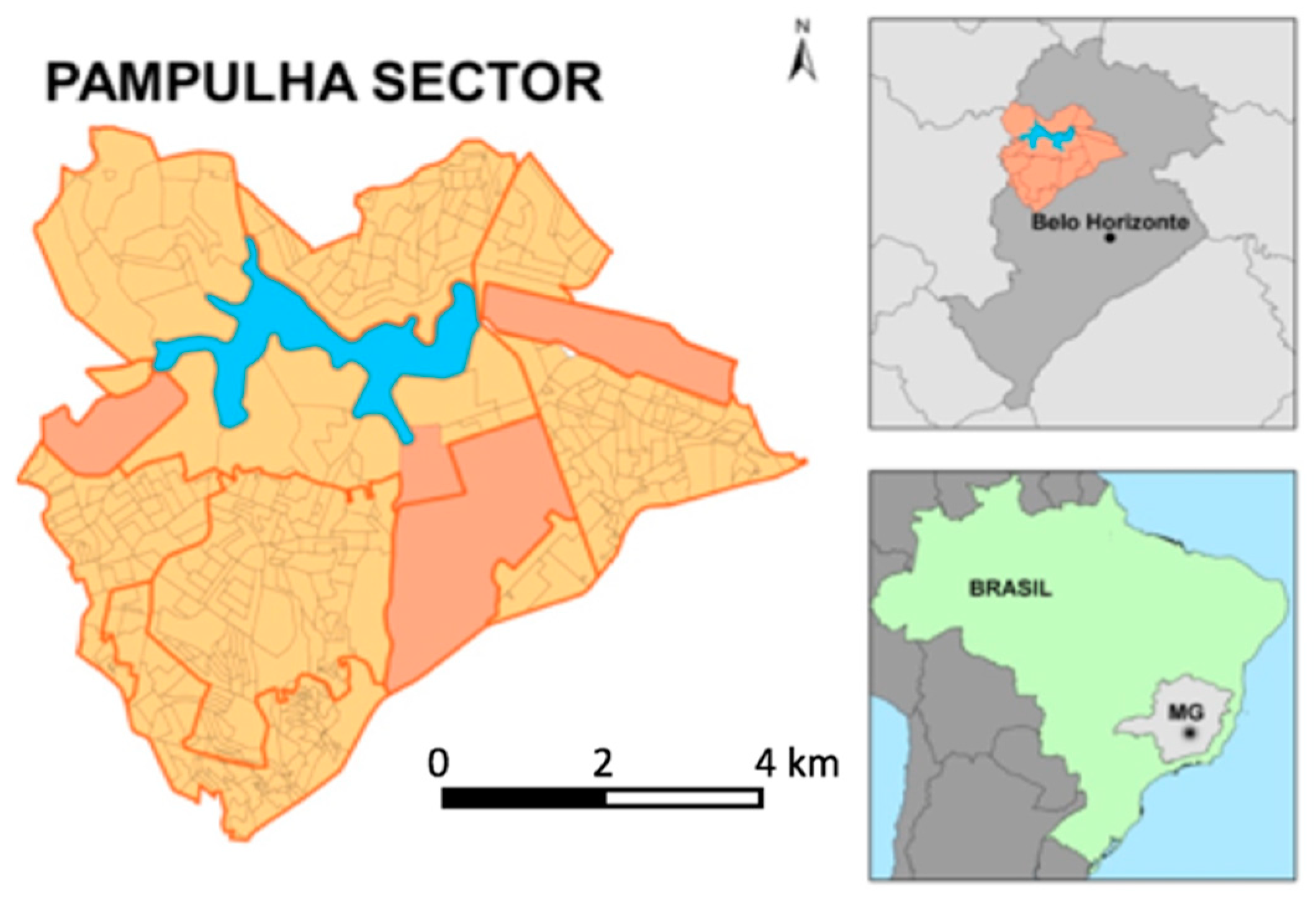
The case study, the district of Pampulha, is known as a very green part of the city but it is also true that these areas are not well distributed, presenting inequalities. Moreover, it is under pressure of transformation, because the area projected by Oscar Niemeyer, the most famous Brazilian architect, was recently declared a World Heritage Site by UNESCO due to its notorious ensemble in which the vegetation cover is part of the genius loci. The position of the district is in the axis of city growth and densification. This explains the importance of the studies and the intention to support the proposal of green infrastructure parameters to the area. (
Figure 1).
The study explores the possibilities of spatial analysis with the support of GIS technologies, going beyond the simple analysis to prove the expected concentration of vegetation cover in areas of high income and low population density, which means that just a part of the population of the city is served by this good condition of green infrastructure. The use of GIS technologies and ESDA methods is a second goal, because the study can be used as a reference for further studies, as exploratory analysis is quite useful to help the researcher to understand spatial distributions and possible correlations.
Green areas in an urban environment have different functions, related to aesthetic quality, areas for socialization and leisure, protection against geotechnical problems, maintenance of aquifers and springs and also to ensure the maintenance of the environmental equilibrium related to the climate, the humidity of the environment, air quality and acoustic control [
1,
2,
3]. Recognizing the importance of green areas and the need to plan green infrastructure, the study selected the robust vegetation that interferes more in urban quality when the goal is to compare some anthropic conditions of land use conditions (density and income).
The city of Belo Horizonte, where Pampulha is located, has around 2.5 million inhabitants, from which 145 thousand live in the 47 square kilometers of Pampulha region, what is considered low density in comparison to the rest of the city. Regarding income distribution, together with the South-Center region, it has the higher income of the city. However, as it can often be observed in Brazil, there is complexity in land use, as there are slums with very low income and portions with high density concentration of inhabitants in the area.
The selection of Pampulha was due to its expressive vegetation cover in comparison to the conditions of Belo Horizonte municipality area. The green areas are robust because of its environmental characteristics of gentle relief and declivity but also due to its formation history—it was projected by Niemeyer to be a reference of modernistic urban ensemble, with the contribution of Burle Marx, an important landscape planner.
Pampulha is just an example of interest to be presented but the same methods can be applied to any urban areas. Green areas are inseparable from the landscape that makes the cityscape and are related to cultural values and to the identity of a place in a broad degree of significance and coherence [
4]. It is important to quality of life in physical and cultural senses.
The conformation of the original vegetal cover in Pampulha is characterized by a transition from the Atlantic Forest (that is more distributed from the center to the south of the city) to the Cerrado (Brazilian Savanna). The Atlantic Forest is constituted by high trees and dense composition, while the Cerrado is formed by medium size trees more adapted to harsh climates where water is scarce, with a less dense composition than the forest. With the construction of Pampulha in the 40s, with a modernistic style of urban planning, most of the original vegetation was replaced by exotic species, selected by designs of landscape compositions. In this sense, when the green areas of the city are studied, it is not possible to talk about original species but about volume of vegetation in a general sense.
The watershed of The Pampulha Dam, in Pampulha Region, is characterized by a depressed topography in relation to the geomorphological characteristics of the entire municipality of Belo Horizonte. It is a relatively flat area, with low relief, high density drainage and extensive river plains. The geological formation consists of gneiss granite from the Belo Horizonte Complex. Due to the intense weathering, deep soils were formed, however, with separated beds of sandy and clayey with poor cohesion, indicating susceptibility to erosion [
5].
These characteristics also explain the dense vegetation cover, due to water, higher temperatures, flat topography and deep soils. Also because of these good conditions, there was a sprawl of urbanization and densification. The construction of the dam, in 1958, resulted in a “lake,” which fostered the process of urbanization of the area and increased environmental conflicts.
The Pampulha Dam is formed by a body of water inserted in an urbanized hydrographic basin where the irregular occupation and the lack of sanitation and erosion control (mainly in the western portion, in the city of Contagem) caused the loss of approximately 50% of its volume, as well as an intense degradation of the water quality [
5,
6,
7]. Environmental studies reported risks in biochemical parameters, such as cyanobacterial proliferation, including potentially toxic species, presence of heavy metals, eutrophication and low amount of dissolved oxygen in the water [
5,
6,
7,
8]. The problems of the water in The Pampulha Dam can be faced with the control of land use and density, the implementation of sanitation in the areas of low income occupation and the protection of green areas.
Green spaces in urban areas are responsible for helping regulate air quality and climate, reducing energy consumption by countering the warming effects of paved surfaces, recharging groundwater supplies, protecting lakes and streams from polluted runoff and maintaining the environmental balance that affects physical and psychological well-being through the influence of urban stressors and factors, such as overcrowded and polluted environment and reduced social support [
2,
9,
10,
11]. Green areas are reported as the most desired environment for relaxing and recovering from stress and sustaining mental efforts [
12], therefore it is important to have these areas incorporated into the designs of the cities, in an interconnected network of natural areas and other spaces [
13].
The main goal of this paper is, as a matter of fact, the use of a method based on the spatial analysis distribution of this observed condition. The spatial analysis technique used was ESDA (Exploratory Spatial Data Analysis), which identifies the existence of clusters of each land use typology, the existence of distribution patterns, the variety of spatial patterns and, more importantly, the spatial autocorrelation.
This case study, facing the relation between vegetation cover, income and population density with the use of ESDA, reveals spatial connections and tendencies that cannot be ignored, because spatial phenomena spread according to contiguity and neighborhood, changing behaviors, composing tendencies, defining new values and establishing a culture.
In this sense, studies that consider the risks and the tendencies in change to support the quality management in landscape are of great interest. This analysis can favor the understanding of the need for green infrastructure parameters in urban laws to be applied in an index of volumetric vegetation cover and in indexes of permeability per lot, per block and per any territorial unit. Using Moran global indexes, it is possible to understand each territorial unit in the sector, in this case study represented by units of census sectors, as reference to plan policies and projects for local scale in punctual interventions or to plan general projects for a broader area.
Geographic and territorial sciences that deal with the characterization, analysis, simulation of change and the proposals of alternative futures to a spatial composition are increasingly relying on the application of digital spatial models to support the studies of phenomena distribution. Among these geographic sciences are those dealing with physical phenomena but there are also those that investigate anthropic actions on space and the dynamics caused by man and environmental interaction. The concepts applied in this case study can be of wide application, being of interest to all those investigating variables related to anthropic issues (socioeconomic, population, values and cultures); to physical issues (vegetation, landscape typologies and many others); and those that study the relationships between anthropic and physical variables (for example, the relation between population density and vegetation cover and many other possibilities).
Geoinformation technologies have expanded significantly since the middle of the last century, associating knowledge about conceptual logics with the possibilities of representing and testing these logics with the technological support. Parallel to digital tools development, we also observe the developments in regulations and laws that favor the wide dissemination of information and facilitate access to data and applications, as support for planning and design.
As a legal point of view, it is important to mention INSPIRE European normative, that established the SDI (Spatial Data Infrastructure) in Europe and was used as a reference to Brazilian IDE in the scale of national data [
14,
15,
16]. As a result, the access to georeferenced data is becoming possible in Brazil. In addition to that, the existence of free GIS software is a condition to make the use of the technology and methods in all scales possible, even in those municipalities with lack of financial conditions. The expectations for the next steps are the free web platforms, providing not only data but also services, increasing the possibilities for the users [
17].
Spatial studies are always related to the process of analysis followed by synthesis. This means decomposing—composing—recomposing, according to the principles of systemic approach. The logic of producing analysis and synthesis to characterize the territory, to identify potentials and restrictions, has been in use before the advent of IT, based on analogic media. The overlay of maps, with the goal to find suitable areas for the equilibrium between environmental protection and anthropic use for the place, was proposed in the 60’s and called “design with nature” [
18].
The logic of decompose, compose and recompose is in the origin of science, when the investigator identifies the main component variables of a phenomenon or of a spatial occurrence and isolates these variables to study them. To understand the behavior of these variables, the researcher composes with them, to verify the significance of some aspects he observed. Once the behaviors are understood, he recomposes to define the insertion of each variable or of a group of variables in the system, to analyze the impacts of possible changes or transformations. Among the expressive literature about this theme, which is in the base of science, we chose to mention the studies in geography were also developed in the 60’s, in discussions about models in geography [
19].
An important field in science that studies the interrelationships among variables, phenomena, occurrences and territory is the System Approach. It defends that it is possible to isolate parts from the whole but without forgetting the existing relation among the parts. The approach was proposed by a biologist also in the 60’s and it is applied to any spatial phenomena that consider mutual influence in anthropic and physical variables [
20].
Once establishing the conceptual base for investigating and modeling the territory, the development of GIS (Geographic Information Systems) allowed the use of applications with the main known models but also allowed to plan and test new spatial models. To develop a model requires knowledge about logics and the capacity to translate these logics into algorithms. However, we are observing the indiscriminate use of spatial models as Apps (Applications) and GIS tools, just because they are available in software, without controlling the possible applications, limitations and suitability for that use. It is important to remember that spatial studies must begin with a clear definition of objectives, deep investigation about possible ways and the best way to achieve the objectives and tests on spatial models to define terms of use. It is also important to understand the specificities related to spatial analysis [
21].
There are still few studies that approach three-dimensional studies applied to urban vegetation cover, especially using LiDAR (Light Detection and Ranging) associated with the NDVI (Normalized Difference Vegetation Index), in order to support the comparison between built and vegetation volumes to evaluate urban environmental quality [
1,
22,
23].
Particularly in Brazil, this is very new, due to the cost of the data capture and to the lack of technicians that are able to work with geoprocessing tools but mainly because the consciousness about the importance of quality of people’s environment and life is still very incipient in order to consider the importance of this variable in landscapes that are increasingly impacted by the processes of intense anthropization, especially with regard to the vegetation cover in the urban landscape. When the “green” variable is presented in any urban plan, it is calculated in bidimensional values, indirectly considered, as the index of permeability [
24]. The parameters used, when applied by the municipality, are—rate of permeability per lot (a percentage of area that cannot be covered by impermeable materials but it does not really mean it will be vegetated); arborization plans to roads (that defines the need to plant a tree in the sidewalk when the proprietor implements the building); the general analysis that calculates the rate of green areas per inhabitant (that calculates the bidimensional surface of any green, without separating robust vegetation from shrubby vegetation and requires an average of 15 square meter per inhabitant) and the “environmental quota” (that accepts substitutes or compensation to the absence of the green, like rainwater collection box or green walls) [
25,
26]. In this sense, the present study chooses the volumetric values in vegetation as parameter of analysis, in comparison to the others that tell about anthropic use of urban land, understanding that this new parameter makes the difference in urban life quality [
27].
Exploratory data analysis is not a new methodological resource, it can be observed in several works in the field of conventional econometrics [
28,
29]. In the same way, Exploratory Spatial Data Analysis is not new but its use is not well known in urban studies in Brazil, where, except for some big cities, there is no culture of strategic plans and, moreover, there are limitations in using spatial data analysis. In this sense, the Exploratory Spatial Data Analysis can play a role in studies about tendencies and behaviors in urban environments and can be considered an innovative contribution. This article presents conceptual bases about spatial analysis (state-of-the-art), as well as a case study to illustrate the applied methods (state-of-the-design), in order to contribute to new future researches.
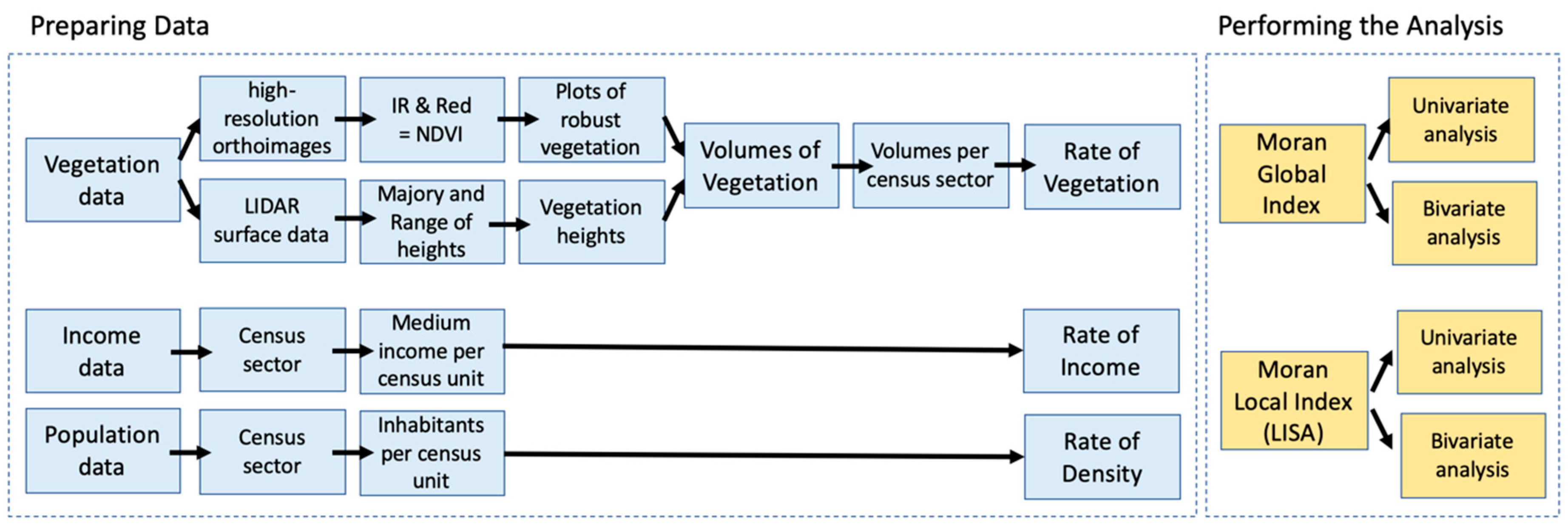
2. Materials and Methods
One of the most important steps in geoprocessing is the definition of the territorial unit to develop the analysis, as space must be discretized in regular or non-regular units. Once representing the space in discrete units, they will be combined in spatial analysis models and in spatial representation. In the example of the present study, it is possible to understand the process of decompose—compose—recompose (
Figure 2).
Initially, reality was represented in regular units of pixels (according to spatial resolution) and in spectral bands (spectral resolution). After this first decomposition, the NDVI (Normalized Difference Vegetation Index) model was chosen to compose the variables. This technique combines red and infrared bands, resulting in an index of vegetation, normalized from −1 to +1 [
27,
30]. Once the model is applied, the representation is recomposed according to the objective of investigation, which means—the identification of areas with robust vegetation cover, woody vegetation. It is also possible to recompose the results according to vegetation levels, from woody to scrubby and grass. In this case study, only the robust vegetation was selected and using the plots of this vegetation, a 3D model was composed, associating the footprints of the trees to the elevation values captured by LIDAR, from the DSM (Digital Surface Modelling). In this sense, we observe that many studies in spatial analysis can be done by processes of decompose—compose—recompose.
The LIDAR data used was provided by the Municipality of Belo Horizonte, captured in 2015. The survey was performed through airborne LASER profiling. The parameters of capture were—FOV angle (field of view) of 20 degrees, flight height of 2388.1 m, stripe width of 1688.1 m, side overlap (between strips) of 36.4%, 76 strips in varied flight directions, with vertical accuracy of 25 cm and average density of 1.5 points per square meter. As the modelling considered the selection of robust vegetation, the number of points was enough to calculate the medium height of the trees, because none of the plots used had less than 36 square meters of projection.
The company responsible for the work performed the pre-processing of raw data and we performed the LIDAR data processing. The pre-processing was basically the use of GPS observations of the base station and of the aircraft, that were initially processed individually and subsequently concatenated in order to obtain a unique kinematic solution and adjusted to a known coordinate system. The first step on LIDAR data processing was also performed by the company, with the goal to separate the points of terrain from the points of surface land use. They used a tool that searches for the points with the lowest dimensions and builds a Triangular Irregular Network (TIN) grid. Most of the times the triangles of this initial model have the sides lower than the terrestrial surface, with few vertices touching the terrain and these irregularities are removed by the program. After that, the program starts modeling the terrain surface, adding more points to the model making it closer to the real shape of the terrain. The points that are added to the model are defined by iteration parameters of angles and distances. These parameters determine how close the points must be to the plane of a triangle to be accepted in the built model.
As the points were provided separated in terrain and surface data, the surface data was selected. They were in Multipoints format and it was necessary to convert to Singleparts to extract all the possible points and keeping the Z value (elevation). Using the shapes of robust vegetation plots, it was performed the Join by Location, which means to extract all the points values only to the projections of the existing trees. Using just the values correspondent to robust vegetation, it was constructed the raster surface model. Applying Zonal Statistics analysis, it was possible to get the Majority and the Range of the elevation values per shape of robust vegetation. The Range was used to control the difference from the lowest to the highest point of the plot element but the Majority value was used to calculate the volume of the vegetation (doing the multiplication of the area of the plot projection by the majority value in the height) [
23,
30].
An important step in the use of models is the definition of territorial unit analysis or spatial integration, that can be vector (decomposed according to graphic primitives of points, lines and polygons) or matrix (decomposed in pixels). In the specific case of neighborhood studies, in which ESDA (Exploratory Spatial Data Analysis) is included, the territorial unit or spatial discretization has a fundamental importance, because it interferes in the definition of what a “neighbor” is [
31,
32].
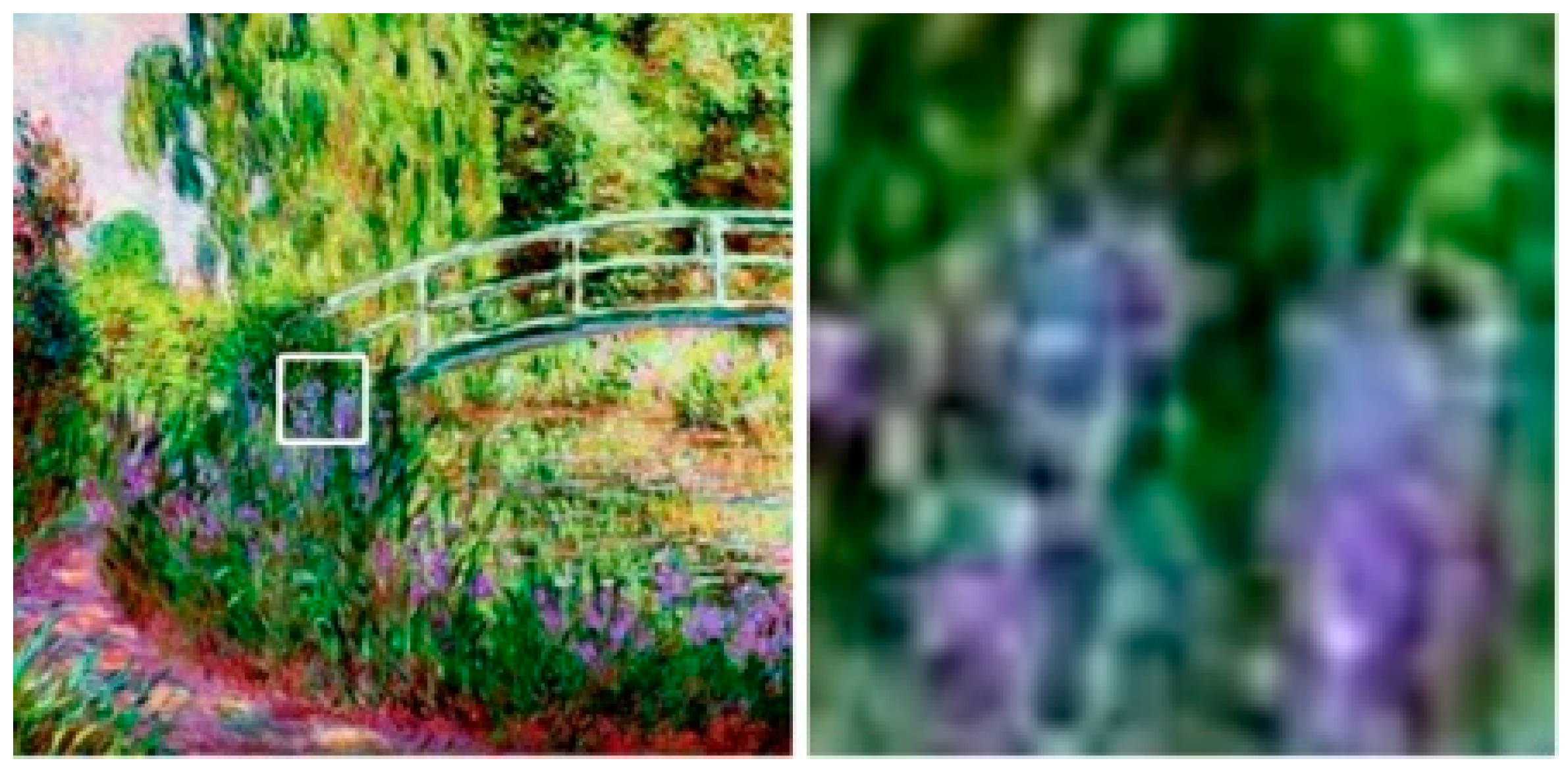
Searching for references in the past, when people were decoding the space into representation types, we can remember the pointillism impressionism (
Figure 3). The question is—how many pixels must be selected from the point of a neighborhood so that the user is able to recognize an element or part of an element? Monet used to say that each color we see comes from the influence of its neighbor. Art had already anticipated the raster logic, that requires two conditions—the discretization of space into small parcels, that represents in spatial analysis the territorial units of integration (that can be pixels or polygons) and the fact that spatial relations are closely related to neighborhood conditions. Considering that elements and their influence in the territory can only be understood and characterized according to their position in the space, it is important to consider this condition while developing spatial analysis and applying spatial models, because it is very important to understand the context in which the elements are inserted.
The definition of territorial units requires also the understanding that spatial parts are linked, to choose the best representation of these connections (
Figure 4). Most geoprocessing models combine different layers that search to answer two main questions—“in this position, which are the characteristics?” or “these characteristics, where are they located?” [
33,
34]. It means that they think vertically, according to the combination of layers in a position but not considering the neighborhood (
Figure 5).
A classic application in spatial analysis is the geographic matrix [
35,
36,
37] and the Multicriteria Analysis [
38,
39,
40,
41] that combine territorial information units (pixels or vector elements) that spatially coincide in a vertical way. The models that consider the neighborhoods must work with horizontal compositions, between elements in the same layer, according to any spatial definition or cutout.
Considering the models that work with neighborhood aspects, they can be separated into those that are used to classify typologies, as the image classification that applies filters or masks (Low-pass filters, High-pass filters, generalizations and groupings); those that work with topologic references (defining conditions of contiguity, connectivity and so on) and those that transform initial data (points or lines) into potential surfaces of spatial distribution of an occurrence or phenomenon (spatial interpolators) [
41].
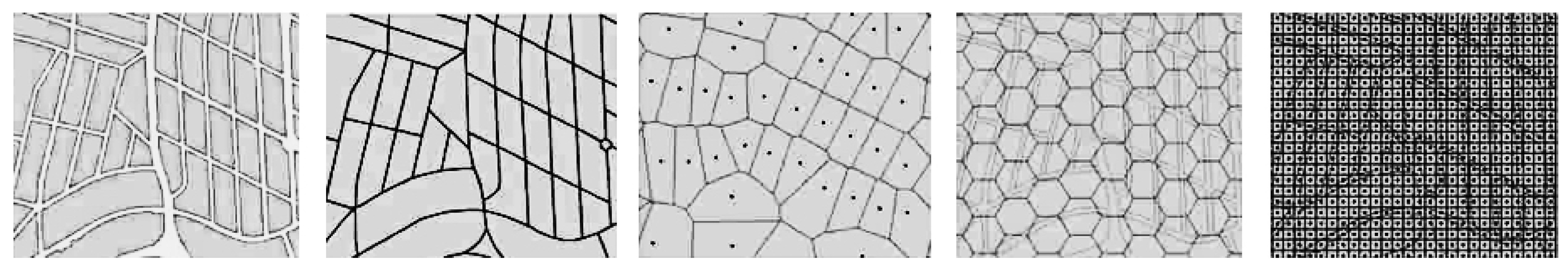
The potential surfaces can be composed by interpolators, each type of interpolators adapted to the behavior or characteristics of the data (if it has regular or irregular distribution), according to the function (if the model is applied to suggest values in parts of the territory in which there were no measures or data or to present the concentration of occurrences). There are many models that must be chosen according to the condition of the data and to the objective of the analysis, as the interpolator of Delauney example (to regular distribution phenomena), the mapping of density using Kernel or of concentration using Clusters (to distribution and concentration studies), the gravitational studies as IDW or Voronoi with friction and mass (to map the area of influence of occurrences), the probability of distribution in a territory simulated by Kriging (considers spatial tendencies and veins), among others. All of them aim to transform data into geographic information, considering the distribution of elements and composing numeric visualization of spatial distribution (
Figure 6).
With the need to consider spatial groupings and the influence from the neighborhood in a process of change and transformation in a city, we must remember the first law of geography, from Tobler—“Everything is related to everything else but near things are more related than distant things” [
42].
The present paper starts from the interest to study urban dynamics and to understand the distribution of life quality in the city, considering the surrounding effects. The variables that were chosen for the analysis were vegetation cover, income and population density distribution. The studies about the general distribution of each variable were done with the global Moran index, which tells if the area is of high value of the variable and the neighbors are also like this, if the area is of low value and the neighbors are also like this, if the area is of high value but the neighbors are of low value or if the area is of low value but the neighbors are of high value.
The studies can be done in a simple variable but also in a combination of variables. In this case, the global Moran index indicates the relation between high/low values of one variable surrounded by values of high/low of the other variable, in the 4 possibilities of combinations. In the case study, the goal was to investigate the relation between the vegetation and income variables, vegetation and population density and of income and population density.
It is also possible to analyze the behavior of one parcel of the territory, using local Moran index, the LISA (Local Index of Spatial Association). The local index allows to investigate, for example, if some territorial units with robust vegetation (woody) are surrounded by similar conditions or by neighbors that are very different in this aspect. This kind of investigation is important because of the risks of following the examples from the practices in the surroundings. The identification of territorial units that have some good conditions but are in the middle of others that do not have the same condition can be an alert to create policies or restrictions to discourage the change.
Also, in local studies, using LISA, it is possible to combine variables and analyze if in one territorial unit there is a good vegetation condition but surrounded by high density population or by low income population or the possible combinations. This kind of study can be strategic to plan the future of the area.
Most of the researches that apply ESDA (Exploratory Spatial Data Analysis) have the studies about equity as a goal. Most of them are interested to know, for example, if the distribution of an infrastructure is spatially coincident with income distribution, because the interest is to prove social inequalities. There are papers about indexes of human development and indexes of economic development or even about the distribution of services and facilities and the relation with incomes and poverty. Most of them are interested in analyzing the asymmetry in the distribution of opportunities [
43,
44,
45,
46,
47].
In the present case study, it is possible to evaluate the equity concerned to green areas and socioeconomic or demographic aspects but the main interest was to use the analysis as a base for strategic studies that consider spatial phenomena that can be influenced by the behaviors of the surroundings. It is the logic that behaviors can conform tendencies, that can construct values that can establish a culture. In this sense, the way of living, the way of using the territory. The research has an innovative use of ESDA, because it is planned to be applied in strategic policies and designs.
The Moran Global (Global Spatial Autocorrelation Index–I-Moran Global) and Local (Local Indicators of the Space Association–LISA) indices were applied in this study using GeoDa software version 1.4.6 [
31,
48]. The I-Moran Global indicates the value of the spatial autocorrelation of a defined variable, regarding the entire data set, explaining if it is spatially concentrated or scattered. The positive values of I-Moran Global (between 0 and 1) mean the existence of direct correlation and the negative values (0 and −1) mean the presence of inverse correlation, functioning as a statistical test in which the null hypothesis is a spatial randomness.
An I-Moran Global statistic indicates a "strength" of spatial similarity or dissimilarity in neighboring regions. If
x1,
x2, …,
xn are places under observation, I-Moran Global for these data is:
where
LISA allows analyzing the spatial association for different locations of a variable distributed in space [
35,
48]. The I-Moran Local statistic measures the spatial autocorrelation of a specific location with its neighbors. Like the I-Moran Global, the significantly positive I-Moran Local indicates that the values of the place in question and its neighbors are similar, that is, there is positive autocorrelation (there are patterns of spatial similarity). The significantly negative I-Moran Local indicates that the value of the location under analysis is unequal in relation to its neighbors, that is, there are patterns of spatial dissimilarity. The Local I-Moran can be calculated for a location
i and when the values of
Ii are different from zero this indicates that the unit
i is spatially associated with its neighbors, according to the equation below.
where
To summarize the steps that constitute the use of techniques related to the methods adopted, it is presented the main workflow of the study (
Figure 7).
3. Results
In order to use the ESDA Model, data from variables must be prepared to represent normalized and numeric distribution. It is not adequate, for example, to use data already segmented in value bands (grouped on discontinuous values) or even in categorical representation (typologies, also known as selective or nominal data). Data must be represented in real numbers, in continuous distribution and must be normalized to allow a comparison in variables.
For instance—if the objective is to compare income with vegetation cover, income cannot be grouped in bands. If we get the absolute numbers, income can go from R$0 to R$9691 (in Brazilian money) and green areas can go from 30 to 9655982 cubic meters (vegetation was associated with the volumetric value of each plot or fragment). To make it possible to compare these different variables, of different natures and with different scales of measurement, normalization is required. When data is normalized, it means that the initial and the last values are the same, while the internal distribution depends on the original distribution of the variable. It is possible to normalize, for example, from 0 to 1, from 0 to 100, according to the users’ decision.
In the territorial units’ decision, green vegetation was characterized by the footprint of the arborous body, the fragment projected in the surface but associated with the values about the volume (data captured from LIDAR and elaborated into volume values). With specific studies that we had done before, in which we were analyzing life quality, the values were grouped by blocks [
23,
30]. The ideal condition was to transform all the variables in distribution per block but in Brazil, socioeconomic data are available only per census sectors, which forced us to work with this territorial unit and to summarize the data from vegetation cover into the census sector unit (that covers many blocks but does not cut a block in the middle, because it respects the limits of the roads).
The neighborhood concept must be very clear when we work with ESDA. It interferes in the preparing of data. If we choose territorial units for the blocks, data must be treated so that the polygons’ faces touch each other, covering the streets and conforming contiguous areas (
Figure 8). In the case of grid representation (the logic of raster, matrix but organized in vectors), this contiguity is clear, because topologic conditions of a neighborhood are explicit but it is not in all cases that this representation can be interesting, as it is a regular grid that presents space as a homogeneous area and does not consider the variances in land cover (as roads, parks). It is also a problem when a variable measured by a zone is converted to grid (pixels) because the user is considering that the value is repeated in all the cells correspondent to that zone, ignoring that values were grouped in the initial representation.
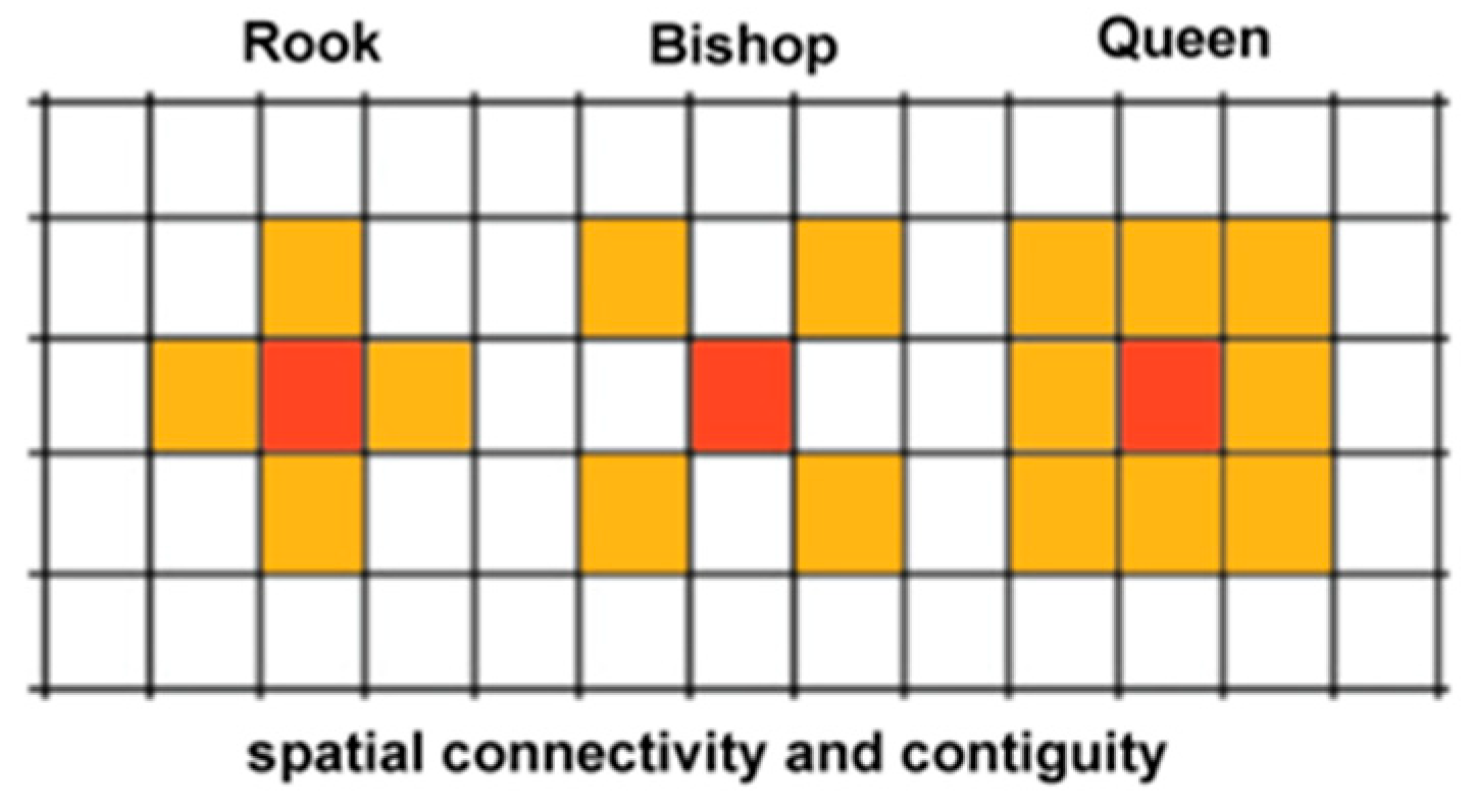
It is necessary to choose the scope of the neighborhood. In the use of ESDA it is necessary to define the relation of rook, bishop or queen. In the matrix of “rook” the neighbors are the cells or elements that have at least one face in contiguity or in contact with the cell or element of reference. In the matrix of “bishop” the neighbors are the elements that have at least one vertex in contact with the element of reference. In the matrix of “queen” the neighbors are those that have at least one vertex or one face in contact with the element of reference. Except for some specific motivation, to meet some objective, the ideal is to choose queen matrix, because it is a broader condition (
Figure 9).
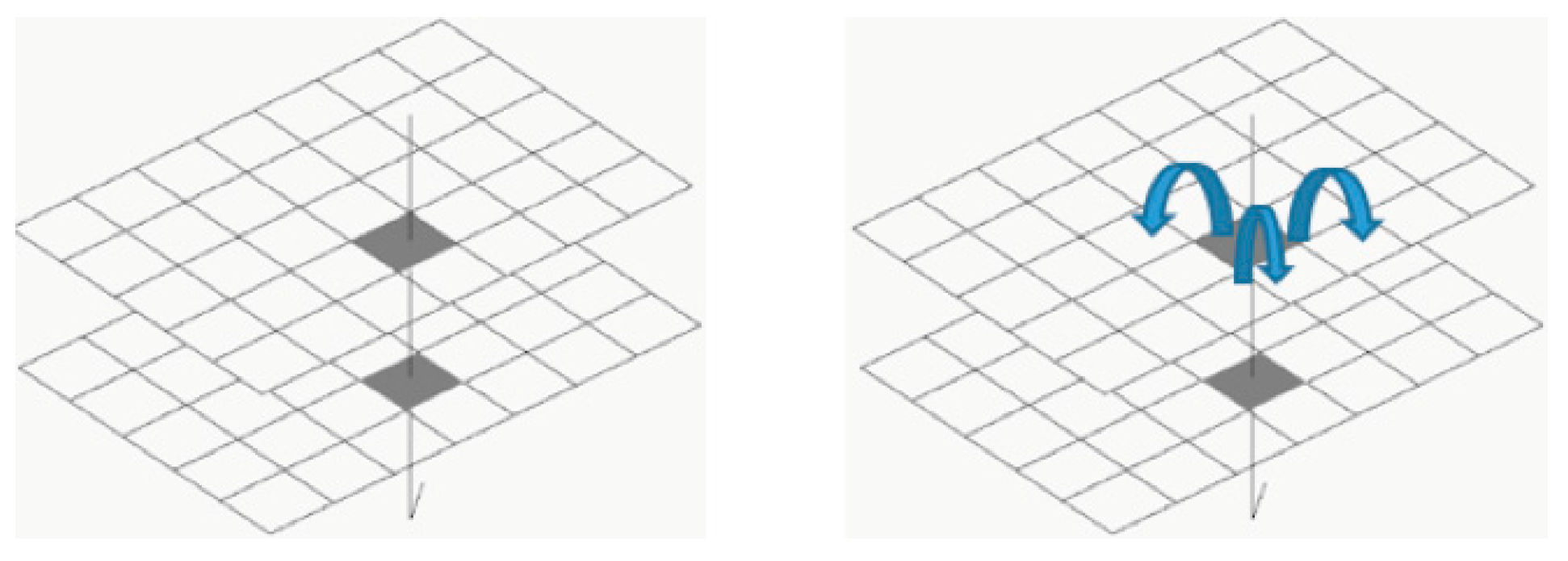
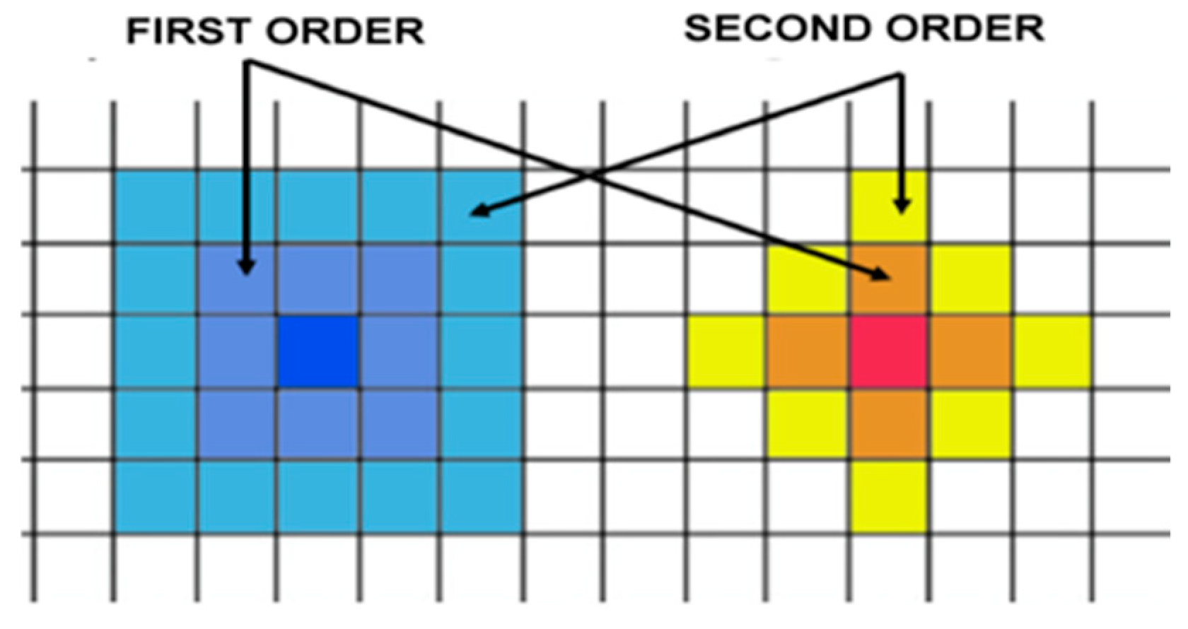
It is important to define the order of interest, that means the maximum number of closest neighbors (k-nearest neighbors) or even the maximum distance from the element of reference. If the k-nearest neighbors are chosen, it is important to define if they are going to be of first order, second order or third order (
Figure 10). The choices are always related to the objectives of the analysis, and, mainly, related to the spatial dynamics of the place.
With the data already prepared and with the relation of the neighborhood already decided, the model is applied. The general Moran index goes from −1 to +1, which means perfect negative spatial autocorrelation and perfect positive spatial autocorrelation. It indicates if there is spatial randomness and presents an index and the visualization of the results in a scatter diagram. The interpretation is based on the direction and slope of the distribution line and by the four quadrants (
Figure 11).
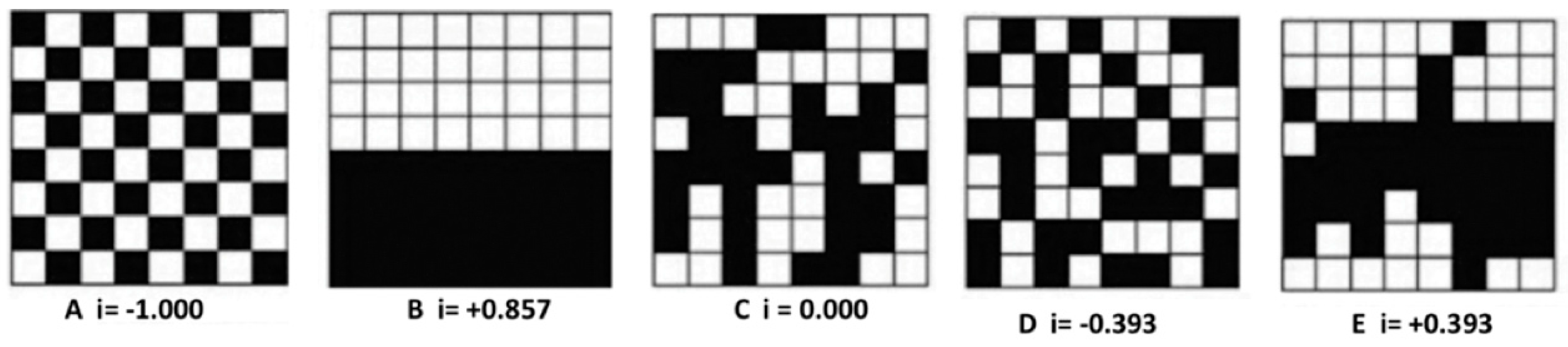
Randomness or autocorrelation interpretation is illustrated (
Figure 12) [
49]. The author explains that in image A, there is a spatial arrangement of perfect negative autocorrelation in Moran index (−1), because each black cell has only white cell neighbors, which means that all the neighbors are different from the cell of reference. In image B Moran index is +0.857, which is a high positive autocorrelation and could be +1 if all the cells were black or all the cells were white. The index was high and positive because in most of the cells the neighbors are the same, except for those in the frontiers of the two groups. In images D and E, we observe equal Moran indexes but one is positive and the other is negative. In the negative index (D), a great part of the image presents spatial regularity, forming a diagonal in which white cells have black cells as neighbors. In the positive index (E), most white cells have white cells as neighbors, which is also true for the black cells and with a spatial regularity in three horizontal lines of concentration. It is also interesting to observe that image C has a Moran index equal to 0 (zero) because there’s no regularity in the distribution, it is completely random, it is not possible to find a spatial logic in the distribution or in the neighborhood.
3.1. Preparing of Data
The first step was to calculate the volume of vegetation cover. Orthoimages with the resolution of 20 cm, divided into the visible spectral bands and the infrared band were used as a source of data. The NDVI (Normalized Different Vegetation Index) was composed to separate the robust vegetation (woody). From the classification, the footprints of the mass of trees were vectorized and fragment polygons of vegetation were composed. With the use of LIDAR data (Light Detection and Ranging), it was possible to get the elevation points and to calculate the vegetation volume from each footprint. The result was information about the volume of robust vegetation.
For the first studies, the values were grouped by block but for the studies in ESDA they were grouped by census sector, because the goal was to compare vegetation with socioeconomic and demographic data, that are made available by IBGE (Brazilian Institute of Geography and Statistics), from the census of 2010. Unfortunately, there is no more updated data on this scale. With all the data in the same territorial unit, the values were normalized from 0 to 1. This step was done in ArcGis©. From that point, a shapefile with polygons of census sectors with the attributes of vegetation, income and population density, all of them normalized from 0 to 1, started to be worked in Geoda [
48].
3.2. Representation of Variables
The first step is the definition of the neighborhood matrix. The “queen” neighborhood was chosen and the level of first order. This means that we assumed as neighbors any census sector that had a vertex or a face in contact with the element in reference and that only the group from immediate proximity (first level) would be considered. This is because the case study, Pampulha, is divided into census sectors of large dimensions, which is different in other parts of the city. In other case studies, it must be considered the need to use a second or third order or even more.
The first maps produced were the distribution of each variable in the area, according to quintile parts (
Figure 13). There are some similarities among the distribution of green areas and income (
Figure 13a,b) and a relation that seems to be the opposite to population density (
Figure 13c). This interpretation is in a general point of view but further investigations can be developed.
3.3. Moran Global Index
The study of Moran global index is applied to the whole territory and has the goal to evaluate the extension of groupings in the entire area, to measure if the grouping is significant, which allows us to think about the possibility of random or not random distribution of the occurrences in the region. The evaluation can be done in a univariate way (only one variable at a time, analyzing its distribution in the territory) or in a bivariate way (analyzing the report between two variables in the area).
3.3.1. Moran Global Index per Univariate Analysis
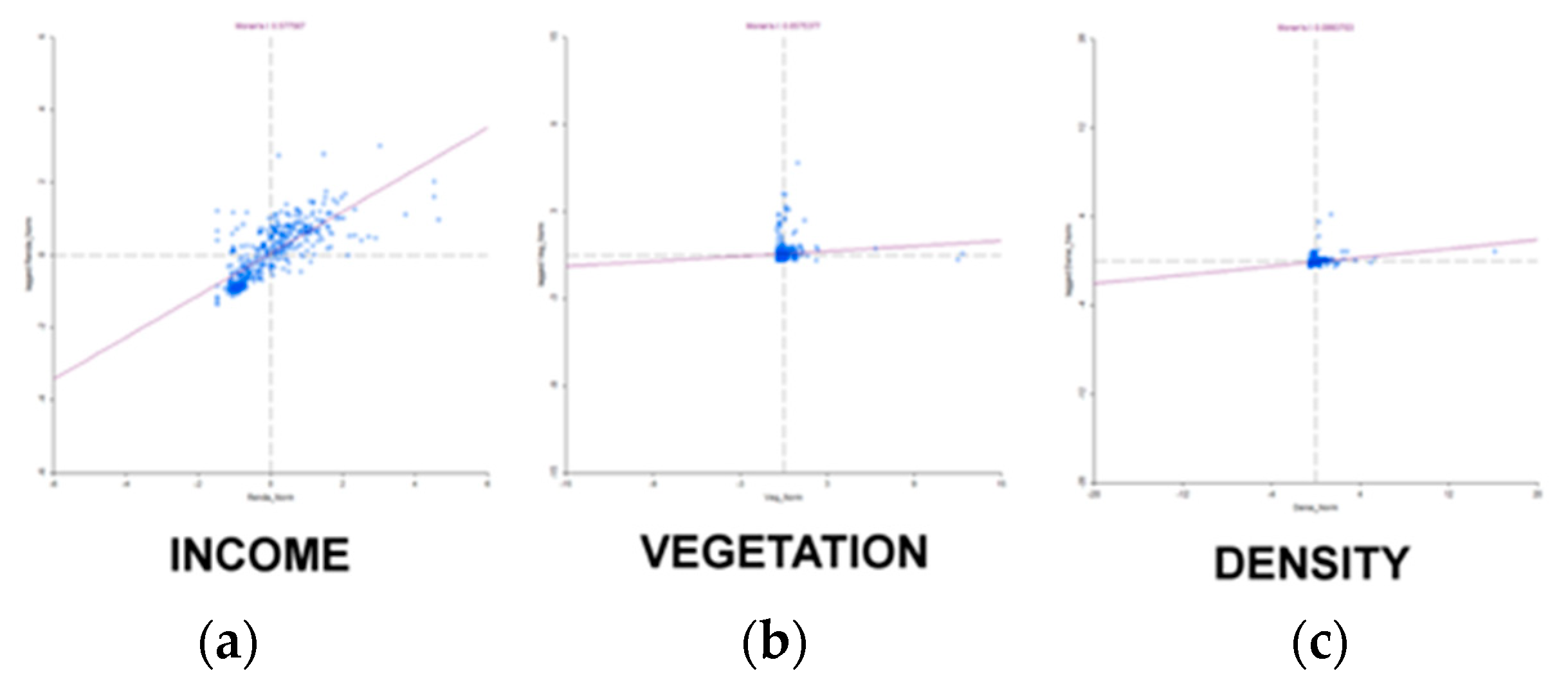
The result of Moran global index for univariate analysis (just the isolated variable) shows that income is the variable that presents the highest positive autocorrelation (
Figure 14a—Moran global index of 0.578), followed by population density (
Figure 14c—Moran global index of 0.099) and vegetation (Moran global index of 0.057) (
Figure 14b). In all variables, there is a positive autocorrelation index, which means that when the variable presents a high level in a part of the territory, its surroundings are also of high values, when there are low values, the neighborhood is of low value. But as all the indexes were not very high, there are also situations of high/low and low/high values. (
Figure 14).
In general, the values of the Moran Global index are not high in the positive sense, which reveals that there is no strong or total similarity between the analyzed phenomenon and its spatial occurrence. However, it is important to note that spatial randomness was not observed for any variable. Values close to zero must be observed, because they mean almost a condition of spatial randomness or spatial independence for the univariate analysis of the population density and vegetation variables. The income variable presents higher spatial correspondence between high values and its surroundings and low values and its surroundings, meaning spatial concentration of social conditions.
On the other hand, the same intensity of the Moran Global index is not observed for vegetation and population density. This means that the variable occurs in space but its spatial pattern of occurrence is tenuous. The result shows that there is not a large spatial concentration of vegetation and population density in the studied region.
3.3.2. Moran Global Index per Bivariate Analysis
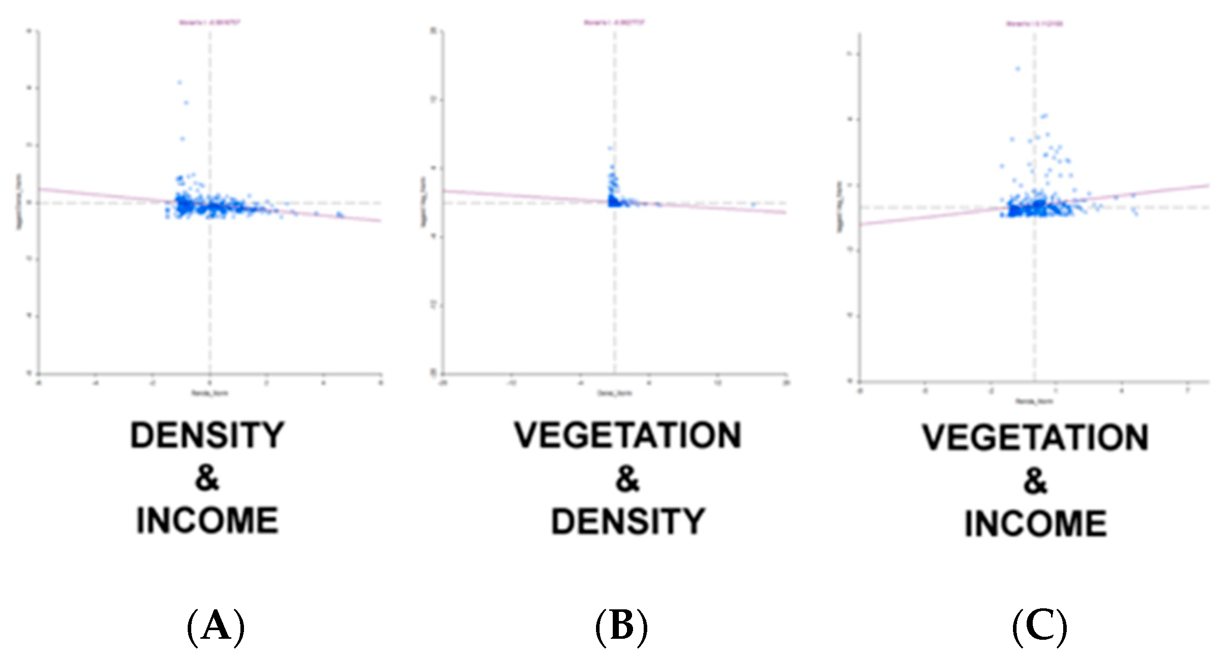
The bivariate analysis evaluates whether there are spatial correlations between variable pairs. Population density was combined with income (
Figure 15A), vegetation with population density (
Figure 15B) and vegetation with income (
Figure 15C), promoting all possible combinations (
Figure 15). The result is that the relation between population density and income presents a negative autocorrelation (Moran global index of −0.092), which means that where income is high, population density is low. The relation between vegetation and population density also resulted as a negative spatial autocorrelation (Moran global index of −0.062), which means that the area is characterized by high concentration of vegetation in areas of low population density. In both cases, the indexes are not very expressive. The index is a little bit more expressive in the relation between income and vegetation, which presented a positive autocorrelation (Moran global index of +0.112).
In none of the autocorrelations the indexes were high, probably because of the high heterogeneity of the area. If some sectors were studied separately, according to homogenous areas, there would be a possibility of achieving higher values. Nonetheless, the indexes confirmed our initial perception and the next step is to study the area in detail, using local indexes (LISA).
Regarding the analysis of the bivariate Moran Global index, the values were close to zero, once again showing a low spatial trend of autocorrelation between the variables. Despite the low values, the expected relationship of negative spatial autocorrelation between population density and income was observed.
In the analysis of population density and the amount of vegetation, there was also negative spatial autocorrelation, showing that the increase in population density puts pressure on the vegetation fragments and their consequent suppression. However, the low value of the Moran index shows the low spatial expression of the relationship, that is, it occurs but it is not spatially evident.
The relationship between vegetation and income resulted in positive spatial autocorrelation, which demonstrates the tendency to preserve fragments of vegetation in areas of higher income and the risk of their suppression in areas of low income. Urban parameters can be used to explain this, since in high-income areas the lots are bigger and proportionally there will be more areas destined for vegetation cover. It was also observed a relationship between low income and the increase in population density and, consequently, greater pressure on vegetation cover.
3.4. Moran Local Analysis
Moran local analysis, LISA (Local Index of Spatial Association), has the goal to evaluate if there are clusters of high values with high values, of low values with low values or even the presence of outliers (high with low values or low with high values). The index also evaluates if these local clusters or the outliers are statistically significant. The results are maps that distribute the values in quadrants (high-high, low-high, low-low and high-low) and identify the territorial units in which the outcomes were not significant (in which there is no defined behavior) and maps that show, in the territorial units that presented expressive results in the previous step, how significant the result was. The studies can be done in univariate or in bivariate mode.
3.4.1. LISA—Moran Local Index, Univariate Analysis
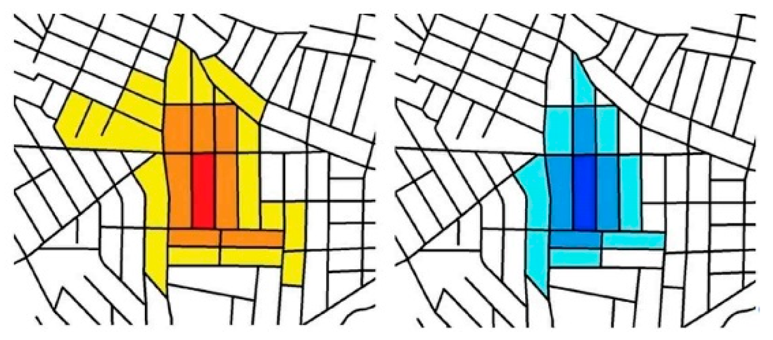
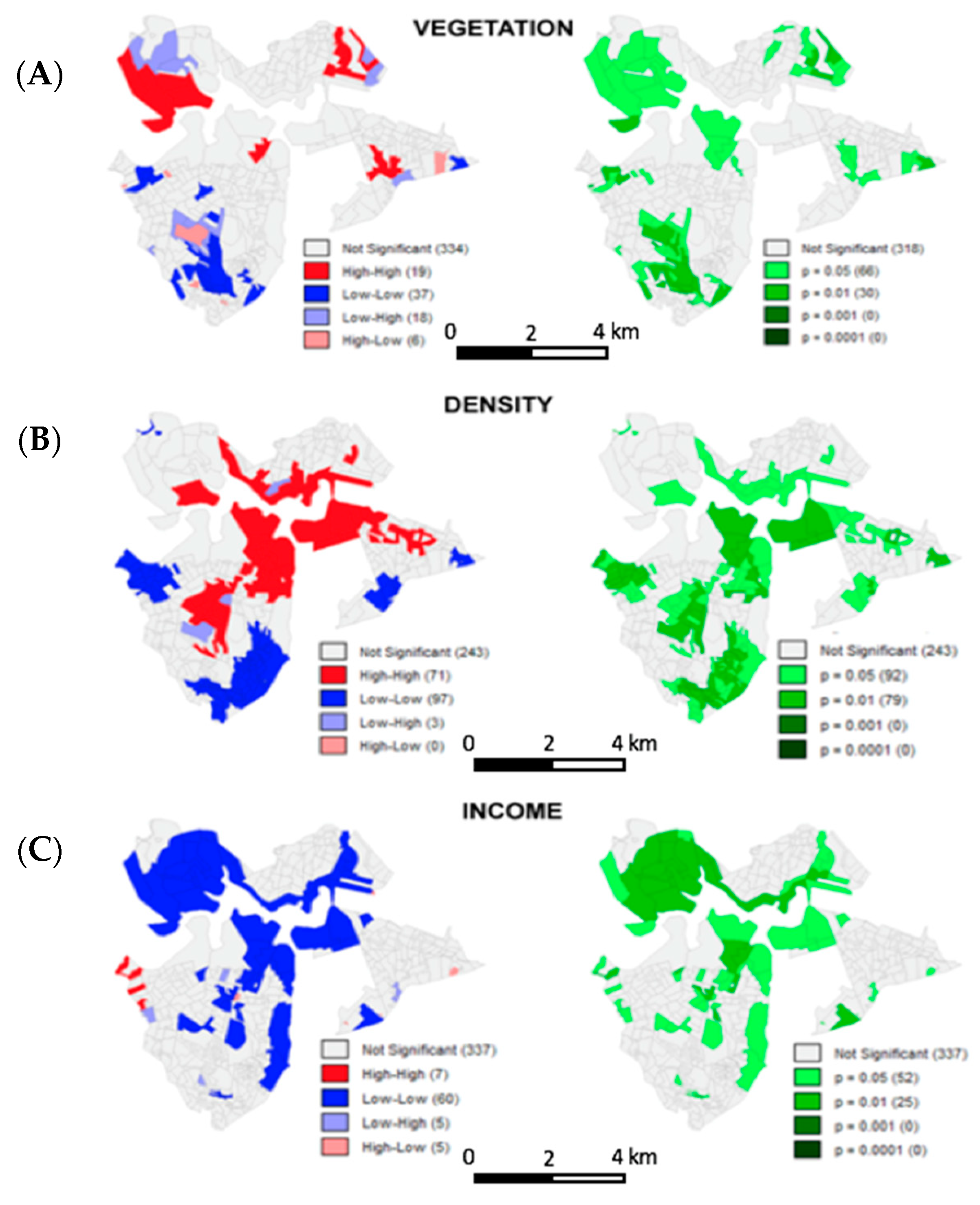
In the case study, it was observed that the income variable presented spatial autocorrelation in two portions of the area, presenting territorial units of high income with neighbors of high income (red, high/high) and units of low income with neighbors of low income (blue, low/low). There are no situations of high income associated with neighbors of low income and there are very few units with low income in areas of high income and the existing ones are slums (light blue, low/high). Analyzing the significance of the observed combinations, the majority is high or medium to high, which supports the results of the analysis. However, most territorial units do not present positive spatial autocorrelation. Two agglomerations of high income and of low income in the area are observed but in the rest of the area there is a lot of heterogeneity. (
Figure 16A–C).
The vegetation distribution analysis (
Figure 16A) presents an expressive number of territorial units with non-significant autocorrelation but it also presents two areas quite defined—a high vegetation level with neighbors with the same condition and another area of a low vegetation level with neighbors of a low level. The areas with low vegetation values call our attention, surrounded by areas of high values. In this case, investments in policies and projects can be done to these areas, so that they can follow local trends and make efforts to improve vegetation cover. Most of the classifications present a high significance.
In the population density analysis, the distribution that stands out is the presence of territorial units of low density inserted in neighborhoods of low density (
Figure 16B) and an expressive number of units where there are no significant spatial autocorrelation and the spatial distribution is random. The significance of the results where spatial autocorrelation was observed is medium high to high.
3.4.2. LISA—Moran Local Index, Bivariate Analysis
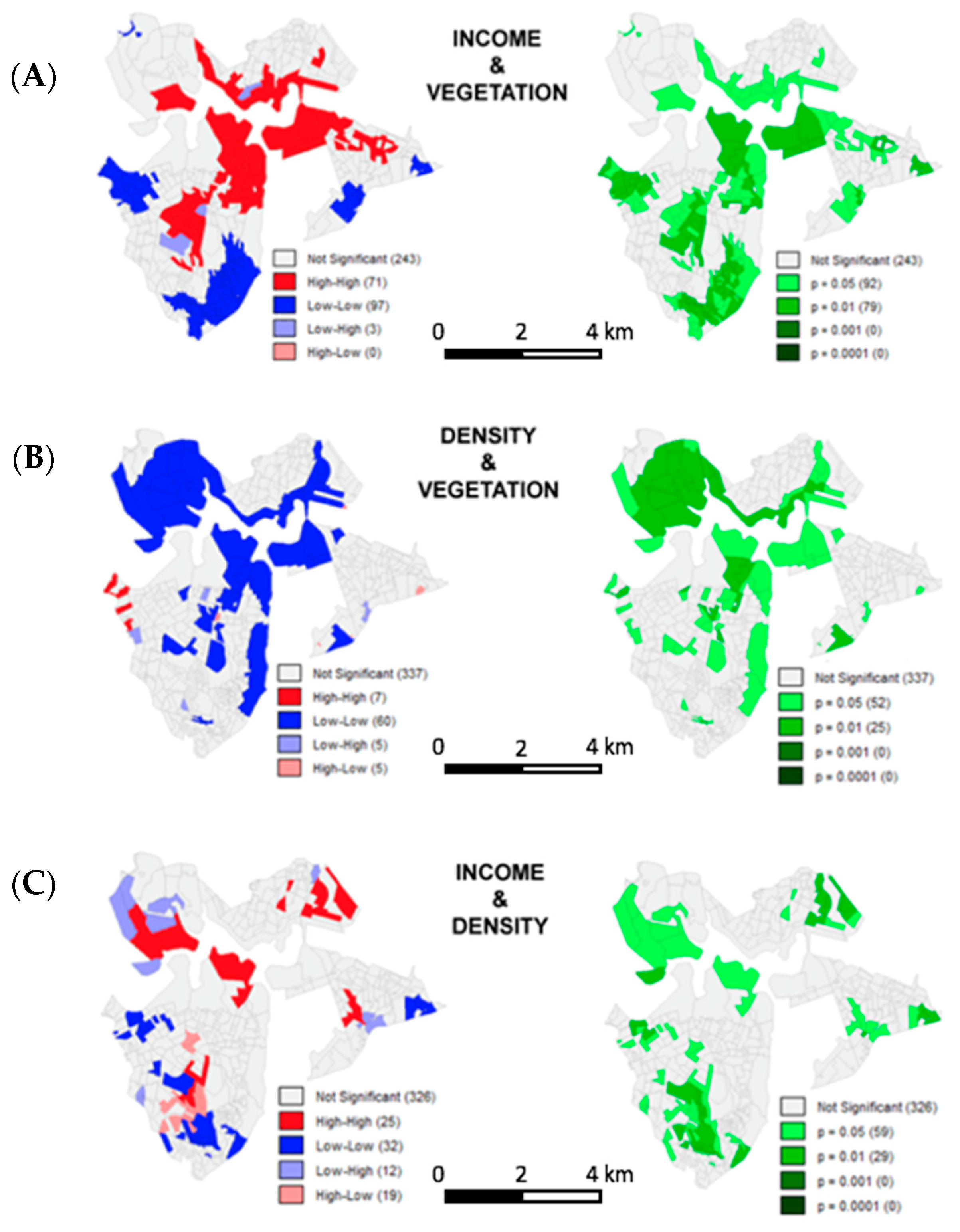
The comparison between income and vegetation resulted that, even though we had many territorial units with non-significant results, there are parts of the area with high income surrounded by parts of high vegetation cover and parts with low income surrounded by parts with low vegetation cover (
Figure 17A) and these two combinations presented significant results. This means that yes, the high income is associated with high presence of vegetation and low income is associated with low presence of vegetation cover.
4. Discussion
The first analysis about LISA bivariate, comparing income and vegetation, made us have the interest to investigate if population density was also correlated, in a negative sense, with vegetation cover (
Figure 17B). The result is an expressive number of territorial units without autocorrelation, with non-significant results but there are parts of the territory with low population density surrounded by neighbors of high vegetation cover and parts of low population density with neighbors of low vegetation, both with significant results.
Pampulha is predominantly a low-density and very green area of the city. This is part of its genius loci and must be considered in public policies and in the management of land use of the area. The relation between income and population density shows that what predominates is the autocorrelation of high income surrounded by low population density followed by low income surrounded by low population density, with a level of significance from medium to high (
Figure 17C).
From the analysis developed, it is possible to affirm that Pampulha has an expressive number of territorial units without spatial autocorrelation, with random characteristic compositions. However, from maps and indexes interpretation it was also possible to see that big zones in the area, especially those composed by big parcels, present significant spatial autocorrelation. These autocorrelations result in the main image of the area, its genius loci, which is expressive vegetation cover, low population density and high income. In face of these characteristics, it is important to maintain this quality of urban environment but also to create policies and projects that can extend this quality to the sectors of low income. It is also very important to observe the risks of transformation into high population density, because, if it happens, it will certainly change the genius loci of the area.
The main limitation about applying ESDA is related to existing limitations in spatial analysis in a general sense—the definition of territorial units of analysis and the aggregation of data, considered scale (resolution) and form (regularity) [
50,
51].
The territorial unit is a reference to collect, organize and analyze data. The ideal reference is a regular grid with high resolution, which means the discretization in very small portions of land cover. There are references to better define this resolution, that has to do with cartographic precision of the base map or of data capture. The smallest territorial unit is the minimum dimension of data capture or the resolution of 0.5mm in the scale of the base map, according to cartographic standard accuracy of class “A” maps [
52,
53]. As an example, using a base map produced in the scale of 1:5000, the minimum element can be 2,5m. Nevertheless, sometimes the users define the minimum grid value according to expectancy of territorial analysis, which means minimum spatial information. As an example, if the user needs to interpret the results by lot or block, he can use a regular grid measuring 10 m or 100 m.
In ESDA it is important to define not only the spatial resolution but also if it is possible to use a regular grid, because it depends on how the data was collected. The better the data collection was distributed, the more precise the analysis will be. Regular grids, considering also the importance of neighborhood definition, can be proposed in tessellations that cover the area of study and consider possible connections from spatial locations. In some cases, it is not possible to use a regular grid, because the data was captured and summarized according to territorial sample units that follow geographic references. Examples of these irregular grids are the use of blocks, districts, census tracts and municipalities. It is possible to convert these very irregular polygons into ones that reduce complexity but keep the proportional distribution of areas, considering a central point of the original polygon. Using the centroid of the original polygon, Thiessen polygons can be designed, with the goal to generalize spatial representation but keeping somehow the report of spatial dimension and neighborhood contacts.
In the case study discussed in this paper, data about vegetation cover was produced from images of high resolution, regular grid of pixels. It was possible to develop a very detailed analysis but the goal was to explore the relation through income and population density to vegetation cover, to predict vulnerabilities and potentialities to the maintenance of this value and to give support to policies in territorial management. Unfortunately, in Brazil, socioeconomic data about income and population are available summarized in census tracts and that defined the spatial resolution of the analysis.
In some cases, as it generally happens in Brazil, the definition of these irregular tracts follow administrative goals (the number of questionnaires by census taker) and not geographic goals (limits and regular dimensions of polygons) and result in lack of precision and possibilities of misunderstandings results. However, there is a possibility, in the future, to work with a better spatial resolution for data collection, by street segment, which will allow different aggregations and a more detailed interpretation.
5. Conclusions
The case study resulted as a useful instrument to work with quantitative and qualitative approach, because it presents the quantitative support to demonstrate a perception that inhabitants from Belo Horizonte have about the district of Pampulha. This makes the analyses supported by defensible and reproducible criteria.
The exploratory studies of spatial data have been used for over one decade in research about socioeconomic aspects, mainly to prove lack of distribution of facilities in the territory, which is being called equity. The contribution of this paper is to focus on the role that a neighborhood can have in behavior factors related to collective conscious or non-conscious decisions.
We defend that the observation of what is happening in the surroundings has an impact on the adoption of values and this can result in increment or decrement of common conditions of life quality to the group. We believe that behaviors produce tendencies, tendencies create values and values structure culture.
Observing those areas in the neighborhood that keep the vegetation cover is an incentive to adopt this practice as a value or as culture but it is important to say that policies and public projects must help to face the challenges of low income and the risks of population density growth. To plan policies and designs, it is very useful to observe each territorial unit, to identify those that have potential to receive interventions, according to their characteristics and neighborhoods. The expectation is that those units have the potential to spread the effects of an intervention, as catalysts, so that from punctual actions we can have effects of irradiation of results. With that knowledge, with less we can do more.
It is also important to consider the limitations and potentialities about ESDA studies. As ESDA is a model, represented from a mathematical and geometrical logic, it is a point of view, a simplification of reality. A model reduces the complexity of reality according to conceptual values, to methodological delimitation, to temporal restriction and to spatial delimitation. As a model, ESDA will never cover all of the reality complexity but it is a point of view. It works as a support to understand occurrences and phenomena, to make the users convert data into information and information into knowledge.
As it is “exploratory,” the goal is to make users change references and parameters to test the behavior of main variables and to test the connections between variables. The main purpose is to provide a tool to explore decision making, considering generalizations. It must be understood as a relative reality portrait and not as an absolute index or report. If the model is understood just as this support to explore the behavior of variables, it is very useful in spatial analysis, mainly to decide about green infrastructure in urban planning.
The importance of identifying zones and spatial typologies is very clear to studies in physical geography, because it is the base of geographic classifications, applied in landscape descriptions and in spatial taxonomies. However, the awareness about this aspect of neighborhood is of interest, particularly, to research about behaviors and social values, because of spatial diffusion and spread of conditions, in which some parts of the territory influence its neighborhoods, which results in dynamic transformation. This means to identify behaviors that can result into tendencies that can construct new values that, already installed, will form a new culture (
Figure 18). As a further development of this study, it is planned to understand what people think about green areas and how green infrastructure is seen in their daily life, with the goal to increase the behavior, tendencies, values and culture about environmental resources, as “nimby” behavior (
Not In My Back Yard, expression to describe opposition to certain controversial projects or those that may be harmful to the environment) is still something to be overcome.


