Article

Performance of Alternative Estimation Procedures of the Implied Equity Duration in a Small Stock Market

1
Facultad de Empresa y Comunicación, Universidad Internacional de La Rioja, 26006 Logroño, Spain
2
Facultad de Ciencias Empresariales, Universidad de Huelva, 21002 Huelva, Spain
*
Author to whom correspondence should be addressed.
Sustainability 2020, 12(5), 1886; https://doi.org/10.3390/su12051886
Submission received: 23 January 2020 / Revised: 19 February 2020 / Accepted: 26 February 2020 / Published: 2 March 2020
(This article belongs to the Special Issue Financial Risk Management and Sustainability)

Abstract

:
This paper is focused on the measurement of interest rate risk of nonfinancial firms. The measurement is the initial step in the risk management, which, in the context of financial risks, it is expected to lead to better levels of enterprises’ financial sustainability. Concretely, we checked the performance of alternative estimation procedures of the implied equity duration as a measure of the exposure to interest rate risk of firms listed on a small stock market. Previous evidence in the US stock market shows that when the implied equity duration is computed using industry-specific parameters instead of market parameters, significant differences arise in their absolute and relative values and even in their ranking. In this paper, we checked the robustness of these results when we moved to a smaller stock market. To do so, we replicated previous analyses carried out in the Spanish stock market but using alternative estimation procedures. We conclude that significant differences arise in the implied equity duration estimations when we consider industry-specific parameters instead of market parameters. This finding in a small stock market is in line with previous evidence found for the US stock market.
JEL Classification:
G12; G14; M41

1. Introduction

The measurement of financial risks is the core of their management, which is essential to achieve the necessary financial security that guarantees the sustainability of the enterprises and contribute to the sustainability of the economic growth. In this context, this paper focuses on nonfinancial firms’ interest rate risk measurement. Concretely, our research is based on the concept of implied equity duration (IED), initially proposed by Dechow, Sloan, and Soliman (DSS) [1].
The IED is a measure of equity interest rate risk developed by adapting the well-known expression of Macaulay bond duration. DSS [1] show evidence that there is a significant association between the IED and the earnings-to-price ratio, the book-to-market ratio, and the sales growth rate, but not to capitalization, thus excluding the presence of a size effect in line with [2]. Their results support the relation of IED-related effects with the Fama and French high-minus-low (book-to-market ratio) factor [3], suggesting that the latter is subsumed in an IED-related factor.
However, as conceded by DSS [1], improvements in their procedures should lead to more accurate and useful estimates of the measure. Concerning this, Fullana, Nave, and Toscano [4] estimated the DSS [1] implied equity duration measure for the US market, but using industry-specific parameters for forecasting and discounting the future cash flows of listed firms as opposed to the market-estimated parameters used previously by DSS [1]. These authors showed that when they move to IED estimations based on industry-specific parameters, significant differences arise in absolute, relative, and rank terms. They also provide evidence that their more refined procedures improve the ability of the IED to measure stock price risk.
Fullana et al. [4] sought the source of this improvement in the context of the market asset-pricing model. These authors found that industry-specific IED better captures all the components of stock price risk in this valuation model, and, as it is expected, higher differences in the duration estimations imply higher improvements in price risk measurements. Furthermore, their results show the highest improvements by using industry parameters-based IED when the original IED has poor performance. Thus, they concluded that the cost of being parsimonious in estimating firms’ duration is high on average and also quite variable across firms, both quantitatively and qualitatively. Moreover, this cost is large enough to reverse the duration-based ranking order of firms and to result in estimated durations without the ability to measure price risk.
In the context of small stock markets, we only found in the previous literature one article in which the DSS [1] approach is applied: Fullana and Toscano [5] computed and analyzed the IED of the Spanish listed firms. Concretely, they estimated the IED for the nonfinancial companies listed in the Continuous Market of the Spanish Stock Exchanges at the end of 2011. In their work, they compared their results with those of DSS [1] for the US market, performed sector and size analyses, and looked for the relationships of the IED with other variables commonly used as firms’ price risk proxies. The authors used the exact DSS [1] methodology to compare their results with the evidence reported by DSS [1] in the context of the US stock market.
The aim of this paper is to check whether the effects, both qualitative and quantitative, of using industry-specific parameters when computing the IED of US firms also occur when we compute the IED of firms listed in a small stock market. Our central hypothesis is that, in a small stock market, there is less variety in the firms listed and perhaps the parsimony of DSS [1] procedures may actually result in greater precision in the IED estimates, or at least sufficient for adequately ranked listed companies To achieve it, we built this paper on the Fullana and Toscano [5] research by applying to their data new procedures to estimate the parameters involved in IED computation as in [4].
We also performed an industry analysis and a size analysis of the differences between and within these firms’ subsamples that arise when we apply the two alternative procedures. To conduct these analyses, we used the industry allocation of firms made by the Spanish Stock Exchange and the composition of Spanish Stock Exchange size indices. Finally, we determined whether the new IED (IEDn) maintains the relationships that IED has with alternative variables used in the previous literature as firms’ price risk proxies.
Our results support that the evidence found by Fullana et al. [4] in the US stock market is also in a small stock market as the Spanish. The use of industry-specific parameters instead of market parameters leads to significant changes in the firms’ IEDs. These changes are large enough not only to modify the ranking the relative risk among companies based on duration but to modify their own risk profile. On the other hand, we also observed that the differences between the IED and IEDn induce significant changes within industries that have a significant impact on the industry analysis by increasing the differences between industries. However, the results show that differences found in the size analysis and in the relationships with alternative variables are not significant.
The rest of this paper is structured as follows. Section 2 is devoted to presenting the implied equity duration developed by DSS [1] and the industry-specific procedures introduced by Fullana et al. [5], and also to describe primary data, the multivariate outlier detection process and the time-series procedure to estimate the autocorrelation coefficients. In Section 3, we conducted the analyses and discuss the results. Section 4 presents the main conclusions.

2. Materials and Methods

2.1. Alternative Estimations of Implied Equity Duration

The history of duration concept takes us back to the seminal work of Macaulay [6]. He defined it “as the weighted average of the time until bondholders should receive the cash flows promised by a bond”. This concept has been the cornerstone of the fixed-income portfolio and bank interest rate risk management [7,8]. Hicks [9] came to the same concept computing the semi-elasticity of bond prices to their yield to maturity. However, while prices of basic coupon bonds only depend on a unique risk factor (their yield-to-maturity) [10], equity valuation is more complex as it includes many risk factors, among which are interest rates, which affect both future cash flows and the discount rate applied in the equity valuation [11].
This is the main handicap, but not the only one, to get an analytic definition of equity duration. Perhaps because it is not straightforward, in the literature we found some authors who approached this concept through the “stock duration” [12,13,14] that was computed for individual firms later by Leibowitz, first in [15], and then in [16,17,18,19,20,21].
In this context, DSS [1] proposed their implied equity duration measure but using the Macaulay’s duration framework. They grouped equity cash flows by maturity into an initial finite period and a subsequent terminal period. Then, they assumed that the actual value of the terminal equity cash flows is the difference between present value of the finite period cash flows and the market capitalization. Thus, the following expression for the IED arises:
I E D = t = 1 T t C F t ( 1 + r ) t P + ( T + 1 + r r ) P t = 1 T C F t ( 1 + r ) t P
where CFt are the future firm cash flows for the finite period (0,T], P denotes the market capitalization of equity, and r is the expected return on equity. As DSS [1] showed, to compute a firm’s cash-flow forecast for period t, we need forecasts of the firm’s return on equity (ROE) and the firm’s equity growth rate (EGR) in period t, and the book value of equity (BV) in period t–1, since:
C F t = B V t 1 · ( R O E t E G R t )
Based on previous results of Stigler [22], Penman [23], and Nissim and Penman [24], DSS [1] modeled ROE as a slowly mean-reverting process:
R O E t = α · R O E t 1 + ( 1 α ) · r + ε t
where α is the ROE long-run autocorrelation coefficient and r is the long-run mean of ROE.
On the other hand, based on the results in [24], they used the sales growth rate (SGR) as a proxy for EGR, forecast from an autoregressive process of first order:
S G R t = α · S G R t 1 + ( 1 α ) · g + ε t
where α’ is the SGR long-run autocorrelation coefficient, and g is the long-run mean of SGR.
Note, as Fullana et al. [4] did, that the IED estimation per se does not require market parameters. However, DSS [1] used for all firms the same historical market averages of ROE and SGR estimated autocorrelation coefficients and the same historical market averages of return-on-equity and GDP growth as proxies of the long-run autocorrelations and long-run means, respectively. As DSS [1] acknowledged, this approach “while parsimonious, is relatively crude”. Thus, “improvements in the procedure should lead to more accurate and useful measures of equity duration”.
Fullana et al. [4] focused their analysis on the measurement of the quantitative and qualitative impact of using industry-specific parameters instead of market parameters in the forecasting and the discounting procedures to compute IED. They estimated industry-specific autocorrelation coefficients of ROE and EGR using pooled data of ROE and SGR over the sample period. In addition, they used the expected cost of capital and growth for a portfolio of firms estimated by the method developed by Easton and Sommers [25] to compute their long-run means.
Fullana et al. [4] highlighted that their “goal is not to find the most accurate estimation of the IED, but to show that by using industry-specific parameters, you can achieve a more accurate estimation of the implied equity duration than by using market parameters”. Therefore, the authors explicitly assumed model risk biases in their expected cost of capital and growth estimations. They also argued that the selection of the “Easton and Sommers [25] estimation method of the implied cost of capital” is because, in their opinion, “it has all the features needed to achieve their objectives and produce results comparable with those of DSS [1]: (i) it is an industry-level method; (ii) it estimates the implicit cost-of-capital and expected growth simultaneously; (iii) it does not require any forecast as input; and (iv) it does not require realized data in addition to those used by DSS”.
The Easton and Sommers [25] methodology permits to estimate the price-implied expected cost of capital and expected growth based on current accounting data from the following regression relation:
E P S t E P S t 1 = δ 0 + δ 1 · P t B P S t B P S t 1 + ε t
where Pt is the price per share of the firm, EPSt is the earning per share and BPSt is the book value per share in period t. δ0 = r is the estimation of the implied cost of capital, and δ1 = (r − g)/(1 + g).
These industry-specific parameters permit modeled ROE as a process that reverts to the industry long-run expected cost of capital, and EGR as a process of the SGR that reverts to the industry long-run expected EGR, both with industry-specific autocorrelation coefficients. Therefore, four industry-specific parameters are needed to forecast each firm’s cash flows.
Fullana et al. [4] used all the firms in the sample to also compute, through the Easton and Sommers [25] methodology, the expected cost of capital and growth of the whole market, which they then used as constant long-run rates in DSS [1] procedures. They noted that this fact effectively avoids the criticism that differences in industry-specific estimations with respect to the estimations à la DSS “are simply a product of the way in which the expected return and growth” are measured. Finally, they also used estimates of the industry cost of capital from the Easton and Sommers [25] method as industry-specific discount rates.

2.2. Data

In Table 1, the sample selection procedure is summarized in Panel A, and the financial variables and data sources are shown in Panel B. For the purposes of comparability with the Fullana and Toscano (2014) results, the initial sample we used includes all nonfinancial firms with accounting data available, listed in the Continuous Market of the Spanish Stock Exchanges at the end of 2011, for a total of ninety firms. Cross-section accounting data at the end of 2011 and 2010 were obtained from Compustat Global Vantage. Specifically, we collected data for the following financial variables: Book value of equity, earnings before extraordinary items, and firm sales. From Bolsas y Mercados Españoles (BME), the operator of all stock markets and financial systems in Spain, we obtained each firm’s end-of-year capitalization for 2011.
From this data, we computed firm-specific ROE and SGR. Figure 1 shows the pair of ratios for each of the ninety firms. Then, we removed twenty-eight outside atypical values of these pairs of ratios, which are selected by the minimum covariance determinant method for multivariate outlier detection as performed by Verardi and Dehon [26]. Our final sample included sixty-two firms, whose pairs of ROE and SGR are shown in Figure 2.
From BME, we also obtained the industry classification of firms in the final sample. The sixty-two nonfinancial firms were grouped into five industries: Oil and Energy (6), Commodities, Industry, and Construction (16), Consumer Goods (24), Consumer Services (11), and Technology and Communications (5). We also use the composition of BME indices constructed by firms’ capitalization, among other factors, IBEX 35, IBEX MEDIUM CAP, and IBEX SMALL CAP, to classify a subsample of forty-six firms by capitalization into large (eighteen firms), medium (eleven firms), and small (seventeen firms). IBEX indices are selective, so not all the listed firms are included in them. Panel C of Table 1 summarizes these classifications and their intersection.
We used Compustat Global Vantage data from 1991 to 2011 to estimate both the ROE autocorrelation coefficient and the SGR autocorrelation coefficient of each of the sixty-two firms included in the final sample and with at least ten consecutive years of available data, using equations (3) and (4). Then, we computed the industry-specific parameters as an average of the available firm-specific coefficients of firms belonging to each sector. Similarly, we computed the overall sample parameters as an average of all available firm-specific coefficients.

3. Results and Discussion

To compute IED using Equation (1), we started by estimating the required four forecast parameters. In Table 2, we show r—the long-run equity return, and g—the equity growth rate, estimated by cross-sectional regression for the overall sample using Equation (5). Next, we conducted the same estimations for each industry with the aim of computing the IEDn. We can observe outstanding differences in the long-run equity return between industries, and between industries and the overall sample. There are three industries that have an r-value close to the overall sample value: Oil & Energy, Commodities, and Consumer Services. However, one of the industries, Consumer Goods, has an r-value close to half the value of the overall sample, and another one, Technology, has an r-value close to twice the value of the whole sample. The implied equity growth estimates show more variability among industries and correctly cluster them depending on their growth-value feature.
Table 2 also shows ROE and 
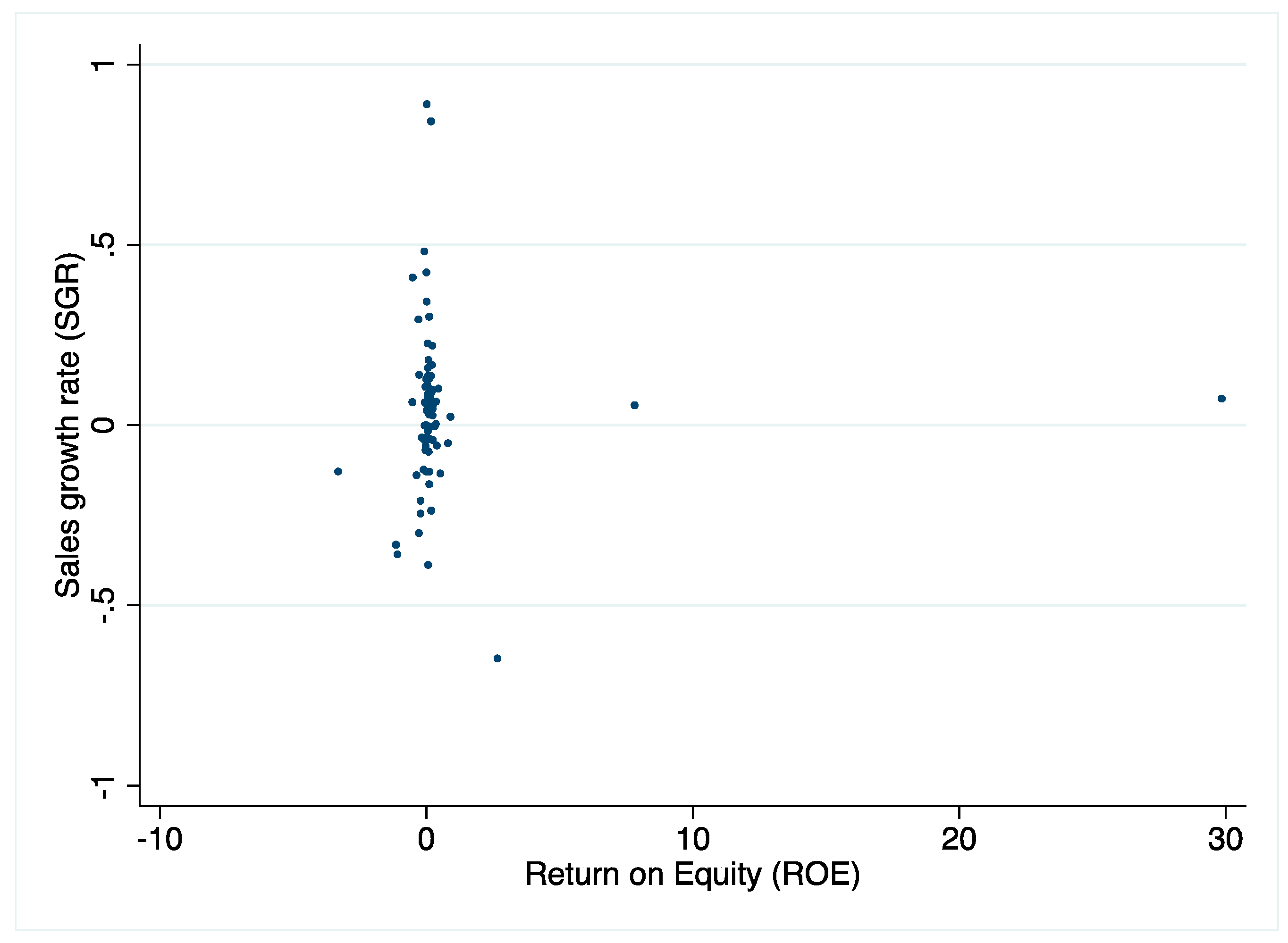
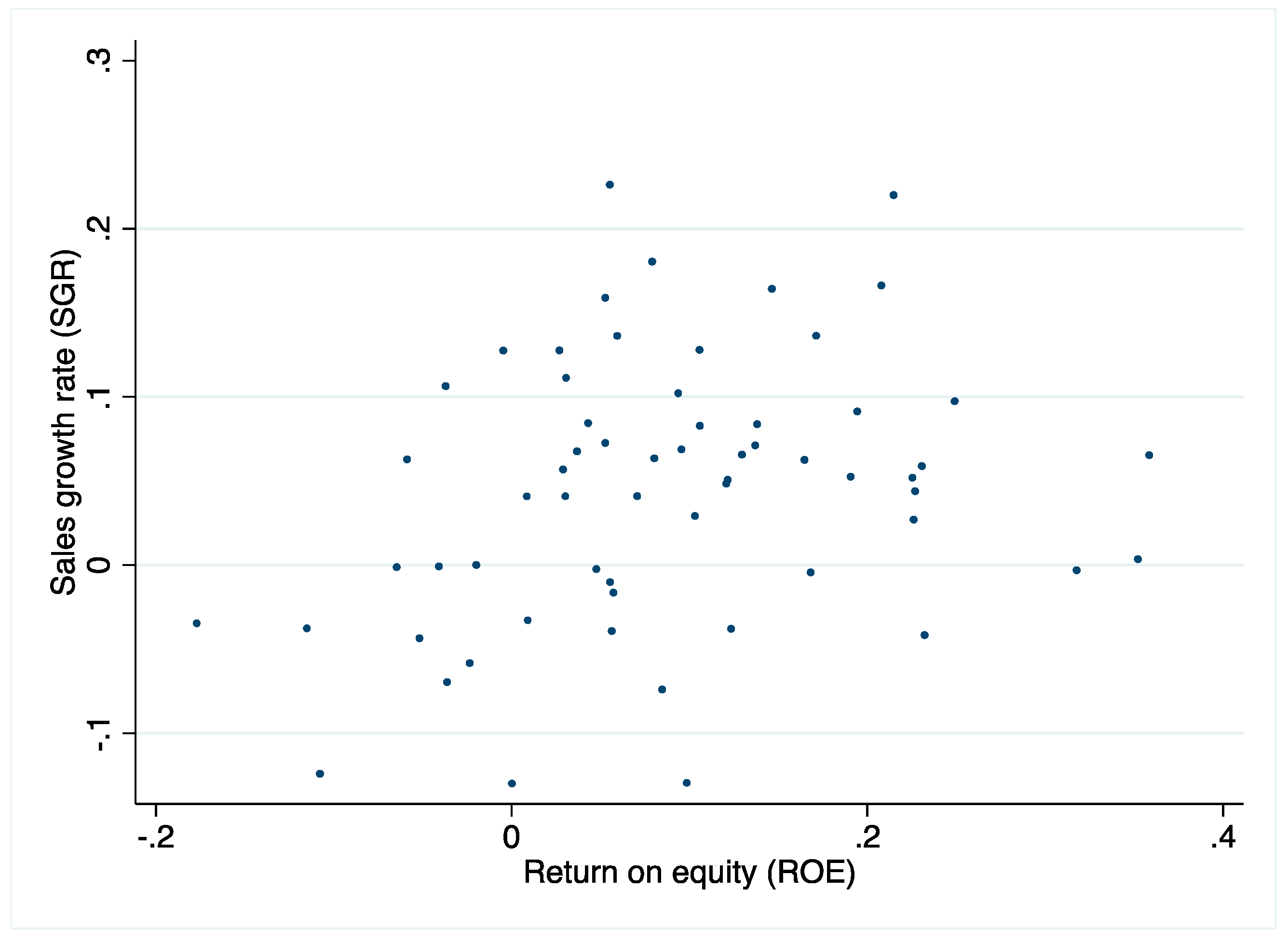
SGR autocorrelation coefficients for the overall sample and each industry. They are averages of time-series estimations of firms performed as we have detailed in the previous section. In this case, important differences also appear around the overall sample values. These parameters set the speed of the firms’ cash-flow reversion to their long-run means, so that equity duration values are very sensitive to them, i.e., a small difference may result in an important variation in the equity duration estimate.
For all the sample firms at the end of 2011, we computed the IED à la DSS using the whole sample parameters, and the IEDn using industry-level parameters. As DSS [1] and Fullana et al. [4], we used a 10 years prediction time period, allowing SGR and ROE to revert to their means. Panel A of Table 3 shows the summary statistics for these results. In the same panel, we report the summary statistics of other variables, computed at the same time, which are usually used as risk proxies: the earning-to-price ratio, the book-to-market ratio, the market capitalization and the annual sales growth rate.
The average of firms’ IED is 19.02 years and their standard deviation is 6.33 years. The lowest quartile and the superior one are defined by 16.37 and 1.90 IED values, respectively. Finally, the IED minimum and the maximum values are 1.61 years and 38.95 years, respectively. These results are slightly different from those obtained by Fullana and Toscano [5], also for the Spanish Continuous Stock Market at the same time. The differences may arise through two ways: the first one is that we updated the initial data sample using Compustat Global Vantage, and the second one is that we have used a more restricted outlier detection methodology, which reduces the standard deviation significantly and refines the market implicit cost of equity and growth rate. The IEDn mean is greater than the IED mean by 2.64 years; however, a higher standard deviation arises when the IEDn measure is implemented, showing that it achieves a better capture of variability among industries.
In Table 3, Panel B, we report the Pearson linear correlation coefficients (below the diagonal) and Spearman’s linear correlation coefficients (above the diagonal) between the duration measures and with the other risk proxies. The correlations between the IED and IEDn are positive, but only between 50% and 60%; thus, even though the main statistics of the two measures do not differ too much, their correlation suggests that they are actually two different measures. On the other hand, the lower correlation of IEDn with these risk proxies than with IED might indicate that the industry-specific measure captures different explanatory risk factors than IED.
The next step in our analysis is to check the effect that the two duration measures produce in the firms’ risk classification based on them. In Table 4, Panel A, we run the analysis by deciles, and we can observe than only approximately 16% do not change decile with respect to the original measure. Thus, in about 84% of the cases, a change in the risk classification of at least one decile occurs. Half of the firms change their risk classification by three deciles or more. In addition, close to 8% of firms change from the lowest five risk deciles to the highest five risk deciles or vice versa.
We also show the results of an analysis by quartiles in Table 4, Panel B. Concretely, we classify firms by their risk level measured by IED and IEDn: from high-risk companies included in the fourth quartile, to low-risk companies when they belong to the first quartile. Between them, we consider companies in the third quartile as those with acceptable risk and companies in the second quartile as those with moderate risk. In Table 4, Panel B, for the full sample, we summarized the quartile changes of the ranges of firms between the IED and the IEDn ranks. This contingency matrix shows that, although 35% of the firms remain in the same quartile, in 65% of the cases, a change of risk quartile occurs. Moreover, in 20% of the cases, the firms change in two quartiles or more. Finally, we observe even one change of three quartiles, i.e., one high-risk company, classified by its IED, is considered a low-risk firm when it is classified based on its IEDn.
In Table 5, we show the summary statistics of the IED and IEDn estimations by industry (Panel A) and by size (Panel B). Concerning industry analysis, we observe that the major differences in the mean appear for Consumer Goods (approximately 10 years), followed by Technology, which is close to (minus) 7 years. Consumer Services has the minimum mean difference of less than (minus) 2 years. Thus, when we advanced to a deeper analysis by sector, the absolute difference that arises between both measures is higher in most industries than for the whole sample. Qualitatively, note that only for the Technology industry the correlation coefficient does not reach fifty percent, indicating a very different rank of firms. For the remainder of the industries, the correlation coefficient between the IED and IEDn are above 90%, so although the quantitative mean differences reported, the firms’ ranks derived from them are quite similar.
When we carried out our analysis by size, the maximum difference occurs for the smallest firms included in the IBEX SMALL CAP, being close to four years on average, while the impact in the largest firms included in the IBEX 35 index is practically naught. In general, results show a quantitative effect lower in the size clusters than in industries. However, from a qualitative point of view, important differences arise. All correlation coefficients, especially the correlation coefficient for the medium firms included in the IBEX MED CAP index, which is slightly less than 32%, are quite low, suggesting that although unrelated to the size, a quite different rank of the firms arises when we move from IED to IEDn.
To check whether differences by industry and by size groups between the IED and IEDn are statistically significant, we conducted a within analysis by medians difference tests. In Table 6, Panel A, in the diagonal, we show by industry the IED and IEDn median differences and, below them, the respective asymptotic significance for the Wilcoxon nonparametric test. All of the median differences are significant at the 1% confidence level, except for the Consumer Services industry, which is not significant. In the diagonal of Panel B, the results by size groups are shown. The median difference is significant at the 10% confidence level only for the smallest firms, and no pattern is drawn by the median differences of the three size groups. This fact corroborates the previous evidence based on correlation coefficients between firms’ duration measures and firms’ capitalizations: When we move from the IED to the IEDn, a clear relation with firms’ sizes does not arise.
To deepen the characterization of the sample firms through their IED versus IEDn, we conducted sectorial and size between analyses in a way that is similar to Fullana and Toscano [5]. This analysis allows us to show evidence of potential firms’ growth options and size effects. Table 6 shows the median differences between industries and indices, followed by the asymptotic significance for the Wilcoxon nonparametric test. Below the diagonals, we show the differences between the group IED medians, and above the diagonals, we show the differences between the IEDn medians. In these results, we can appreciate in a very clear manner that, when we used the IED, the differences between industries shown in Panel A are generally smaller than when we used IEDn. Moreover, most of the differences between industries become significant when we move to IEDn. Concretely, when we used IED, three differences are significant at the 5–10% confidence level, while when we used IEDn, there are six significant differences at the 10%, with five of them at the 1% confidence level. Again, the size analysis results shown in Panel B do not provide evidence of significant differences.
Finally, given the relationships between the IED and EPR and between the IED and BtM that have been analytically proved by DSS [1], and given the previous evidence in [5] that empirically confirms these relations for the Spanish stock market, we performed a cross-sectional regression analysis based on our previous correlation analysis between the IED and IEDn as dependent variables and the EPR, the BtM, and the SGR as independent variables, including CAP as a control variable. Table 7, Panel A shows the results for the IED regression. As in [5], the significance of the BtM and SGR in explaining the IED is significant, and CAP is not likely because the BtM withdraws its effect, as noted by Chen [2]. However, now the EPR turns out not to be significant, which is probably related to the use in this work of a new initial database and a newfangled outliers’ detection. When we moved to IEDn, the explanatory power of the independent variables decreases with respect to IED, and the EPR is close to being significant at the 10% level. In these regression results, shown in Table 7, Panel B, the expected signs remain invariant, but BtM and SGR are less significant, suggesting that the IEDn is a more orthogonal risk measure to the independent variables than the IED.

4. Conclusions

Based on Macaulay bond duration, the implied equity duration was developed by Dechow, Sloan, and Soliman [1] in their seminal paper with the aim of capturing an important common risk factor in stock returns. However, their measure has been underutilized in the subsequent literature, perhaps because as they estimate it, the measure did not have significant added value in financial valuation and risk analysis. Recently, Fullana, Nave, and Toscano [4] demonstrated that, when we move to an industry-specific estimation approach, significant differences arise in the estimates in absolute, relative, and rank terms. Fullana et al. [4] also provided evidence for the US stock market that their procedures improve the performance of the implied equity duration to capture stock price risk and its two components in the market model, the market risk and specific risk.
This work also focused on analyzing the effects of using the industry-specific estimation procedures in the computation of the implied equity duration, but for the nonfinancial companies listed in the Spanish stock market. We are simultaneously interested in the robustness of both the Fullana et al. [4] results when we move to a smaller stock market and the Fullana and Toscano [5] results for the Spanish stock market when we move to an industry-specific estimation approach. We conducted a sector analysis and a size-groups analysis and took a close look at the differences between and within these firms’ groups for both estimation approaches, as originally applied and adapted for the industry-specific case.
Our results show significant changes in the implied equity duration of the firms listed on the Spanish stock market when we moved to the industry-specific approach that manages to change the firms’ risk classification. These results are in line with the previous evidence for the US stock market and, in same way, question the previous implied equity duration estimations for the firms listed on the Spanish stock market. Our regression results also confirm both the poor relation between firms’ sizes and durations for the Spanish stock market and the most relevant fact that, when we move to an industry-specific estimation approach, the implied equity duration becomes a more orthogonal risk measure with respect to other usual price risk measures.
Regarding the size analysis, the results confirm the light relation between firms’ sizes and durations shown by the regression analysis, but the low correlation coefficients found suggest that the industry-specific estimation approach results in an actual new duration measure. On the other hand, the industry analysis shows how the industry-specific estimation approach induces more variability among industries. However, the high correlation coefficients between the two duration measures within industries suggest that, as Fullana et al. [4] claimed, more accurate estimation procedures can be applied to capture more of the firms’ variability within industries.
For all that, we can conclude in favor of the use of industry-specific estimation procedures in the computation of the implied equity duration, also in the small markets such as the Spanish stock market. This better measurement of the nonfinancial firms’ interest rate risk will contribute to its management, allowing enterprises to achieve better levels of financial sustainability.

Author Contributions

All the authors contributed to the conceptualization, formal analysis, investigation, methodology, writing of the original draft, and writing review and editing. All authors have read and agreed to the published version of the manuscript.

Funding

This research was funded by MINECO | FEDER grant number ECO2015-65826-P.

Acknowledgments

The authors are grateful for the comments and suggestions from Alan Duboisée, Eloise de Jager, Juan M. Nave, Kenneth Roskelley and two Sustainability anonymous referees. The authors also thank feedback from participants in the V World Finance Conference in Venice; XXIII Finance Forum in Madrid; and seminars at Universidad de Castilla–La Mancha, University of Liverpool, University of Leeds, and Mississippi State University. This paper was partly written when Olga Fullana was visiting the Universidad de Huelva.

Conflicts of Interest

The authors declare no conflict of interest.

References

  1. Dechow, P.M.; Sloan, R.G.; Soliman, M.T. Implied Equity Duration: A New Measure of Equity Risk. Rev. Account. Stud. 2004, 9, 197–228. [Google Scholar] [CrossRef]
  2. Chen, H.J. Firm life expectancy and the heterogeneity of the book-to-market effect. J. Financ. Econ. 2011, 100, 402–423. [Google Scholar] [CrossRef]
  3. Fama, E.F.; French, K.R. Common Risk Factors in the Returns on Stocks and Bonds. J. Financ. Econ. 1993, 33, 3–55. [Google Scholar] [CrossRef]
  4. Fullana, O.; Nave, J.M.; Toscano, D. The Implied Equity Duration When Discounting and Forecasting Parameters are Industry Specific. Account. Financ. 2018, 58, 179–209. [Google Scholar] [CrossRef]
  5. Fullana, O.; Toscano, D. The implied equity duration for the Spanish listed firms. Span. Rev. Financ. Econ. 2014, 12, 33–39. [Google Scholar] [CrossRef]
  6. Macaulay, F.R. Some Theoretical Problems Suggested by the Movements of Interest Rates, Bond Yields, and Stock Prices in the United States since 1856; NEBER Books: Cambridge, UK, 1938. [Google Scholar]
  7. Lee, H.W.; Xie, Y.A.; Yau, J. The impact of sovereign risk on bond duration: Evidence from Asian sovereign bond markets. Int. Rev. Econ. Financ. 2011, 20, 441–451. [Google Scholar] [CrossRef]
  8. Duan, J.; Sealey, C.W.; Yan, Y. Managing banks′ duration gaps when interest rates are stochastic and equity has limited liability. Int. Rev. Econ. Financ. 1999, 8, 253–265. [Google Scholar] [CrossRef]
  9. Hicks, J.R. Value and Capital; Oxford University Press: Oxford, UK, 1939. [Google Scholar]
  10. Ferrer, R.; Bolós, V.J.; Benítez, R. Interest rate changes and stock returns: A European multi-country study with wavelets. Int. Rev. Econ. Financ. 2016, 44, 1–12. [Google Scholar] [CrossRef]
  11. Peiró, A. Stock prices and macroeconomic factors: Some European evidence. Int. Rev. Econ. Financ. 2016, 41, 287–294. [Google Scholar] [CrossRef]
  12. Lintner, J. Corporate Growth under Uncertainty. In The Corporate Economy; MacMillan: London, UK, 1971. [Google Scholar]
  13. Boquist, J.A.; Racette, G.C.; Schlarbaum, G.G. Duration and Risk Assessment for Bonds and Common Stocks. J. Financ. 1975, 30, 1360–1365. [Google Scholar] [CrossRef]
  14. Livingston, M. Duration and risk assessment for bonds and common stocks: A note. J. Financ. 1978, 33, 293–295. [Google Scholar]
  15. Leibowitz, M. Total Portfolio Duration: A New Perspective on Asset Allocation. Financ. Anal. J. 1986, 42, 18–29. [Google Scholar] [CrossRef]
  16. Leibowitz, M.L.; Sorensen, E.H.; Arnott, R.D.; Hanson, H.N. A Total Differential Approach to Equity Duration. Financ. Anal. J. 1989, 30–37. [Google Scholar] [CrossRef]
  17. Cohen, R.D. The relationship between the equity risk premium, duration and dividend yield. Wilmott Mag. 2002, 6, 84–97. [Google Scholar] [CrossRef] [Green Version]
  18. Hamelink, F.; MacGregor, B.; Nanthakumaran, N.; Orr, A. A comparison of UK equity and property duration. J. Prop. Res. 2002, 19, 61–80. [Google Scholar] [CrossRef]
  19. Lewin, R.A.; Sardy, M.J.; Satchell, S. UK measures of firm-lived equity duration. Int. Financ. Rev. 2007, 7, 335–347. [Google Scholar]
  20. Shaffer, S. Equity duration and convexity when firms can fail or stagnate. Financ. Res. Lett. 2007, 4, 233–241. [Google Scholar] [CrossRef]
  21. Leibowitz, M.L.; Bova, A.; Hammond, P.B. Real Return Tents and Equity Durations. In The Endowment Model of Investing: Return, Risk, and Diversification; John Wiley and Sons: Hoboken, NJ, USA, 2010; pp. 213–223. [Google Scholar]
  22. Stigler, G.J. Capital and Rates of Return in Manufacturing Industries; Princeton University Press: Princeton, NJ, USA, 1963. [Google Scholar]
  23. Penman, S.H. An Evaluation of Accounting Rate-of-Return. J. Account. Audit. Financ. 1991, 6, 233–256. [Google Scholar] [CrossRef]
  24. Nissim, D.; Penman, S.H. Ratio Analysis and Equity Valuation: From Research to Practice. Rev. Account. Stud. 2001, 6, 109–154. [Google Scholar] [CrossRef]
  25. Easton, P.D.; Sommers, G.A. Effect of analysts′ optimism on estimates of the expected rate of return implied by earnings forecasts. J. Account. Res. 2007, 45, 983–1015. [Google Scholar] [CrossRef]
  26. Verardi, V.; Dehon, C. Multivariate outlier detection in Stata. Stata J. 2010, 10, 259–266. [Google Scholar] [CrossRef] [Green Version]
Figure 1. Return on equity versus sales growth rate for 90 firms in the initial sample.
Sustainability 12 01886 g001
Figure 2. Return on equity versus sales growth rate for 62 firms in the final sample.
Sustainability 12 01886 g002
Table 1. Sample selection, financial variables, and market classifications.
Panel AFirm Sample Selection
Listed firms on 31/12/2011123
Financial sector companies29
Accounting data not available4
Outliers removed28
Number of firms in the final sample62
Panel BFinancial Variables and Database
Book value of equityCompustat
Earnings before extraordinary itemsCompustat
Firm salesCompustat
Market capitalizationBME
Panel CSummary of Final Sample Firms by Size Index and Industry
Industries#IBEX 35IBEX MCIBEX SC
Oil & Energy65--
Commodities16625
Consumer Goods24259
Consumer Services11233
Technology531-
Totals62181117
Data from Compustat Global Vantage and Bolsas y Mercados Españoles (BME). Firms listed in the Continuous Market of the Spanish Stock Exchanges. Industry classification and size indices composition are from BME. Firms in IBEX 35 are selected among the largest listed firms. IBEX (MC) MEDIUM CAP includes selected medium capitalization firms. IBEX (SC) SMALL CAP includes the smallest capitalization selected firms.
Table 2. Forecasting and discounting parameters.
Autocorrelation
IndustriesrgROESGR
Oil & Energy0.07700.07670.35630.9098
Commodities0.07420.01830.51620.8058
Consumer Goods0.04530.02730.52700.8062
Consumer Services0.08580.01940.68840.8745
Technology0.16780.15320.40090.7591
Whole sample0.08810.07630.49770.8311
The long-run equity return (r) and the long-run equity growth rate (g) estimated by cross-section using the Easton and Sommers (2007) methodology.
Table 3. Descriptive statistics and correlations for risk measures.
Panel A. Descriptive Statistics
MeanSdMinMaxQ1MedianQ3
IED19.026.331.6138.9516.3719.8521.90
IEDn21.668.39−1.1843.6316.3920.1027.90
EPR0.050.18−0.990.630.010.080.11
BtM1.241.050.075.570.510.941.52
CAP3.329.290.0361.100.150.481.93
SGR0.050.08−0.130.230.000.050.09
Panel B. Correlations (Pearson/Spearman)
IEDIEDnEPRBtMCAPSGR
IED 0.51700.0800−0.27350.10380.8633
IEDn0.5968 −0.0087−0.2559−0.10540.3628
EPR0.23670.0063 − 0.10330.13410.3241
BtM−0.2365−0.1823−0.4409 −0.5272−0.0865
CAP0.0419−0.0860.0648− 0.1725 0.0283
SGR0.74430.34510.2822− 0.10770.0029
IED: implied equity duration using market parameters. IEDn: implied equity duration using industry-specific parameters. EPR: earning–price ratio. BtM: book-to-market ratio. CAP: market capitalization in thousands of millions of euros. SGR: sales growth rate [(Salest-Salest-1)/Salest-1]. Pearson’s linear correlation coefficients appear in Panel B below the diagonal, and Spearman’s linear correlation coefficients are above the diagonal. In bold, coefficients are significant at 5%.
Table 4. Changes in risk ranking by IED.
Panel A. Ranking by Absolute Deviations between IED and IEDn Deciles
DifferencesFrequencyPercentageCumulative
0 deciles10 firms16.13%16.13%
1 decile13 firms20.97%37.10%
2 deciles8 firms12.90%50.00%
3 deciles15 firms24.19%74.19%
4 deciles11 firms17.74%91.94%
5 deciles4 firms6.45%98.39%
8 deciles1 firm1.61%100.00%
Total62100.00%
Panel B. Changes in Risk Ranking between from IED to IEDn by Quartiles
From / toRisk ranking by IEDn
By IEDHighAcceptableModerateLowObs
High risk572115
Acceptable risk725216
Moderate risk326415
Low risk052916
Obs.1516151662
IED: the implied equity duration with market parameters; IEDn: the implied equity duration with industry-specific parameters. In Panel B, risk ranking is obtained by quartiles, being Q4: High risk, Q3: Suitable risk, Q2: Prudent risk, and Q1: Low risk.
Table 5. Descriptive statistics for IED and IEDn by sector and by index.
Panel A. By Sector#MeanSdMinQ1MedianQ3Max
Oil & Energy621.232.6616.4420.0622.0123.0823.77
(0.9259) 24.654.1019.0521.2824.8728.3129.52
Commodities1618.777.211.6116.2719.0722.6032.82
(0.9249) 16.117.38−1.1815.1217.7920.4124.15
Consumer Goods2417.105.362.1914.2518.5720.5427.33
(0.9681) 26.978.236.5522.1328.6831.1743.63
Consumer Services1120.968.445.6517.5120.9025.9338.95
(0.9530) 19.366.0312.2315.3017.4823.6632.69
Technology522.123.5119.2219.5220.7523.5127.62
(0.4973) 15.451.1514.2314.5915.5215.7417.18
Whole sample6219.026.331.6116.3719.8521.9038.95
(0.5968) 21.668.39−1.1816.3920.1027.9043.63
Panel B. By Indices#MeanSdMinQ1MedianQ3Max
Ibex351820.333.5614.2918.2919.8223.0827.29
(0.5734) 20.706.0512.8715.3019.5426.3031.64
Medium1118.744.1110.9916.3120.3821.3323.51
(0.3178) 21.425.7516.3917.1819.2324.4933.74
Small1717.778.171.6113.3618.9821.1032.82
(0.7180) 21.6811.25−1.1816.9423.6629.4643.63
Whole subsample4619.005.791.6116.3719.8222.0932.82
(0.6207) 21.248.15−1.1816.4420.0826.3043.63
Above, the main statistics of the implied equity duration using market parameters (IED). Below in italics, the main statistics of the implied equity duration with industry-specific parameters (IEDn). Below, sector labels appear in brackets, Pearson correlation coefficients between IED and IEDn. #: Number of observations.
Table 6. Test differences of medians.
Panel A. By IndustryOil &EnergyCommoditiesConsumer GoodConsumer ServicesTechnology
Oil & Energy−2.86617.0786−3.80827.39529.3528
0.00720.00640.27620.05620.0062
Commodities2.93131.2812−10.88680.31662.2742
0.33790.00190.00020.65700.1604
Consumer Goods3.43180.5005−10.106111.203413.1609
0.02580.49010.00000.00860.0086
Consumer Services1.1043−1.8271−2.32763.42491.9575
0.61530.34850.09490.13450.1567
Technology1.2553−1.6760−2.17650.15115.2313
0.99800.24770.04960.77700.0086
Panel B. By IndexIbex35 Medium Small
Ibex350.3565 −0.0082 −4.4417
0.9429 0.4952 0.3614
Medium−0.8023 1.1506 −4.4335
0.6893 0.1633 0.6550
Small0.6000 1.4023 −4.6851
0.5018 0.6893 0.0562
Below the diagonal are the median differences by sectors and indices for IED à la Dechow, followed by asymptotic significance for the Wilcoxon nonparametric test. Above the diagonal are the median differences by sectors and indices for industry-specific IED, followed by asymptotic significance for nonparametric tests in brackets (Wilcoxon). In the diagonal, in italics are the median differences between IED à la Dechow and IED industry-specific for each sector and index.
Table 7. IED and IEDn cross-sectional regression against other corporate risk proxies.
Panel A. IEDCoefficientSdt-Valuep-Value
EPR−2.27243.3770−0.67000.5040
BtM−1.27600.5769−2.21000.0310
CAP0.00000.00000.09000.9300
SGR58.97837.03638.38000.0000
Constant18.02211.035217.41000.0000
Panel B. IEDnCoefficientSdt-Valuep-Value
EPR−9.29186.3226−1.47000.1470
BtM−2.01191.0801−1.86000.0680
CAP0.00000.0000−0.97000.3380
SGR39.678313.17363.01000.0040
Constant23.15461.938111.95000.0000
The coefficients in the table are estimated by linear regression through the equation:
IEDi or IEDni = Constant + b1 ·EPRi +b2 ·BtMi +b3 ·CAPi +b4 ·SGRi +et
The following is the standard deviation of the t-statistic coefficient and its significance. The F statistic obtained for four degrees of freedom was 20.61, the R-squared of 59.13% and adjusted R-squared of 56.26% for IED, and 3.22 (F), 18.43% (R-squared), and 12.71% (adjusted R-squared) for IEDn. EPR: 2011 year-end earning-to-price ratio as annual earnings over market capitalization. BtM: book-to-market ratio calculated as year-end 2011 book value of equity over market capitalization. CAP: market capitalization at year-end 2011 in millions of euros. SGR: sales growth rate as sales annual difference over the previous period sales [(Salest−Salest−1)/Salest−1.

