Temporal–Spatial Distribution of Ecosystem Health and Its Response to Human Interference Based on Different Terrain Gradients: A Case Study in Gannan, China

Abstract

The exploitation, utilization, and protection of land resources are some of the great social problems during the process of rapid urbanization in China. The status of land use directly affects ecosystem health (ESH). The evaluation of ESH and the spatial correlations between urbanization caused by human interference help us to analyze the influence of urbanization on ecosystems and also provide new insight into reasonable and scientific resource management. In this study, we evaluated the ESH of Gannan, in Jiangxi Province, China, based on ecosystem service values (ESV) and selected a series of indicators to detect the impact of urbanization on ecosystem health in 1990, 1995, 2000, 2005, 2010. and 2015. Remote sensing (RS) and the Geographic Information System (GIS) were used as processing tools to calculate basic data and to map the results based on different terrain gradients. The results show that ecosystem health suffered a downward trend from 1990 to 2015. Especially, the area proportion at an unhealthy level and average health (ave-health) level increased prominently, and the area of a well state decreased. Further, the results indicate that urbanization had a negative impact on ESH. The degree of a negative correlation increases with the process of urban sprawl. In addition, we found that from 1990 to 2015, the area proportion of a degraded level and unhealthy level was the highest on the first terrain gradient, and as the terrain gradient increased, this area proportion also decreased. However, the high interference region occupies a higher proportion in the lower terrain gradient. Consequently, the results could reveal the impact of urbanization on ecosystem health and could provide an even more effective service for a sustainable development.

1. Introduction

With the rapid development of urbanization in China, human activities have significant impact on the structure and function of ecosystems [1,2,3], which have caused serious degradation to the ecosystem [4]. At present, how to balance the development of ecosystem health and human interference is the subject of extensive research, including in China [5,6]. The degree of human interference is a measure of human impact on the ecosystem, and its level depends on the extent to which human activities hinder the natural development of the ecosystem [7,8]. The rapid development of the contemporary society and economy leads to urban sprawl, which is thought to be a critical contributor to ecosystem change and deterioration [9]. Therefore, the research on urbanization and the ecological environment system has become a hot topic in the academic field. Fang et al. [10] created the theoretical framework of the interaction coupling effect between urbanization and the ecological environment. Liu et al. [11] revealed the stress effect of urbanization by human activities on the ecological environment and the constraint effect of the ecological environment on urbanization. Thus, the relationship between ecosystems and human interference has become closer [3]. China is currently experiencing the process of urbanization, and this rapid urbanization process will continue to develop in the future [12]. Therefore, it is very important to balance the relationship between urban development and ecosystem health, whereas monitoring the states of ecosystem health (ESH) and analyzing the effects of urbanization on the ecosystem provides an effective way of urban sustainable growth.

Ecosystem health indicates the ability of self-organization, self-maintenance, and recovery from stress over time [13]. Maintaining a healthy ecosystem is the fundamental guarantee for the sustainable development of urban areas, because a healthy ecosystem can provide a material basis and ecological services for human activities and wildlife [14]. Ecosystem health is closely related to human beings, so we need to evaluate ecosystems in a certain way to understand the health status. Many studies have assessed the health of different aquatic and terrestrial ecosystems, such as coastal ecosystems [15] river/stream ecosystems [16], agricultural ecosystems [17], and forest ecosystems [18]. The three most common analytical frameworks for ecosystem health assessments are subsystem evaluation; pressure–state–response (PSR); and vigor, organization, resilience, and ecosystem service (VORS) [19]. Each of the three evaluation models has its own advantage. Early studies focused on the inclusion subsystem, such as the resource-environment-socio-economic composite subsystem [20]. The PSR model focuses on the causal relationship between ecosystem quality and human activities, and selects various indicators for evaluation [21]. Those two evaluation models only consider the external pressure and state of an ecosystem, ignoring the ecosystem service function. Whereas the VORS framework integrates both natural ecosystems and human ecological services, which is a relatively comprehensive evaluation model [19]. In order to obtain scientific and reasonable evaluation results, we need to have a comprehensive and objective understanding of the ecosystem quality, including its function and structure.

Gannan is a typical mountainous and hilly region with abundant forest resources, which has an important ecological function and value in China. Consequently, with the continuous development of urbanization, it is important to further analyze the response of ESH to human interference. The complex topographic conditions lead the changes of ESH and human interference in the whole region to show significant spatial differences. Therefore, we analyzed the problem from the perspective of terrain gradient. In this study, taking Gannan region as an example, the whole region was divided into five terrain gradients, and we analyzed land use/land cover change law, spatiotemporal differences in ESH, and spatial responses to human interference based on terrain gradients during 1990 to 2015. We calculated and processed data collected from 1990 to 2015, and the results were analyzed by hotspot map and spatial clustering. In addition, the results were combined with a terrain gradient map and administrative zoning map for further analysis, which are conducive to improving the designated ecological environment and formulating reasonable regional development policies.

2. Materials and Methods

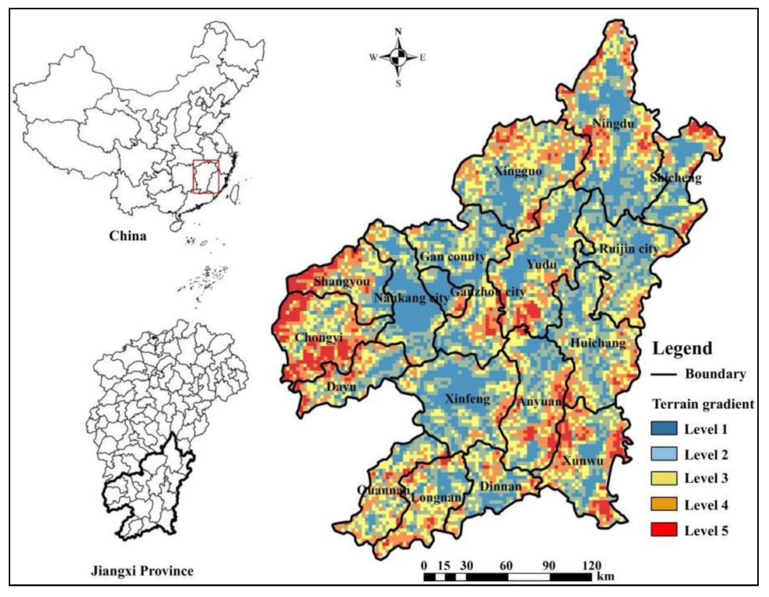
2.1. Study Area

The Gannan region is located in the south of Jiangxi Province, between 24°29′ to 27°09′ N and 113°54′–116°38′ E (Figure 1). The whole area of Gannan is 39,347 km², accounting for 23.6% of the whole area of Jiangxi Province, and is the largest administrative region of Jiangxi Province. The area is rich in resources of forestry, with a forest coverage rate as high as 75%—far higher than the national level at the same time. The rich forestland resources and well protected native ecosystem in this area play an important role in regional climate regulation. This area belongs to the mountainous hilly area. The mountainous hilly area occupies a total area of 80.98%. The terrain is relatively complex, so the development of all counties is quite different. Chongyi County (Figure 1) in the west and some counties in the south have a higher terrain gradient, which is the main distribution area of the forest. The central and northeastern counties have a lower overall terrain gradient and better topographic conditions. The spatial evaluation and spatial clustering analysis on the degree of ecosystem health and human interference in this region can help to identify the areas where human interference and ecosystem health clustering have occurred, so as to optimize the regional development and promote the sustainable development of the regional economy.

2.2. Data Collection

Land use data of 1990, 1995, 2000, 2005, 2010, and 2015 was used for this study. It comes from the Data Center for Resources and Environmental Sciences (The Chinese Academy of Sciences, Beijing, China) (http://www.resdc.cn/). Its spatial resolution is 1 km. The spatial elevation data comes from the Geospatial data cloud (The Chinese Academy of Sciences, Beijing, China) (http://www.gscloud.cn/). Its spatial resolution is 30 m.

In this paper, a 2 km grid [22,23] was used as the basic evaluation unit to calculate the ecosystem health and human interference degree in Gannan. The data were preprocessed using “ArcGIS” (version 10.4) and “Fragstats” (version 4.2) software.

2.3. Methods

In order to analyze the problem based on the terrain status, we classified the terrain gradient in Gannan. Then we used the corresponding evaluation model to facilitate the quantification of indicators. The specific method is described as follows.

2.3.1. Terrain Gradient Classification

The terrain niche index is a topographic value for the comprehensive description of elevation and slope [24]. It can fully display a certain point’s topographic condition and it is usually used to analyze the differences between land use structure and ecosystem health value on various topographic conditions. The site with lower elevation and slope has a lower terrain niche index. The site with high elevation but low slope or with low elevation but high slope has a medium terrain niche index [24]. This study firstly calculated the terrain niche index with the formula in each grid, and then the study area was divided into 5 terrain gradients according to the calculation results and the Jenks natural break method [25]. Terrain gradient level 1 to 5 corresponded to the terrain niche index as follows: 0.2022–0.6972, 0.6972–1.1326, 1.1326–1.5463, 1.5463–2.0312, 2.0312–3.7107 (Figure 1). The terrain niche formula is as follows:

$$T=\ln \left[\left(\frac{E}{E_0}+1\right)\times \left(\frac{S}{S_0}+1\right)\right]$$

(1)

where T refers to the terrain niche index, E is the altitude of a point, S is the slope of a point, E₀ represents the average altitude of the entire study area, and S₀ represents the average slope of the entire study area.

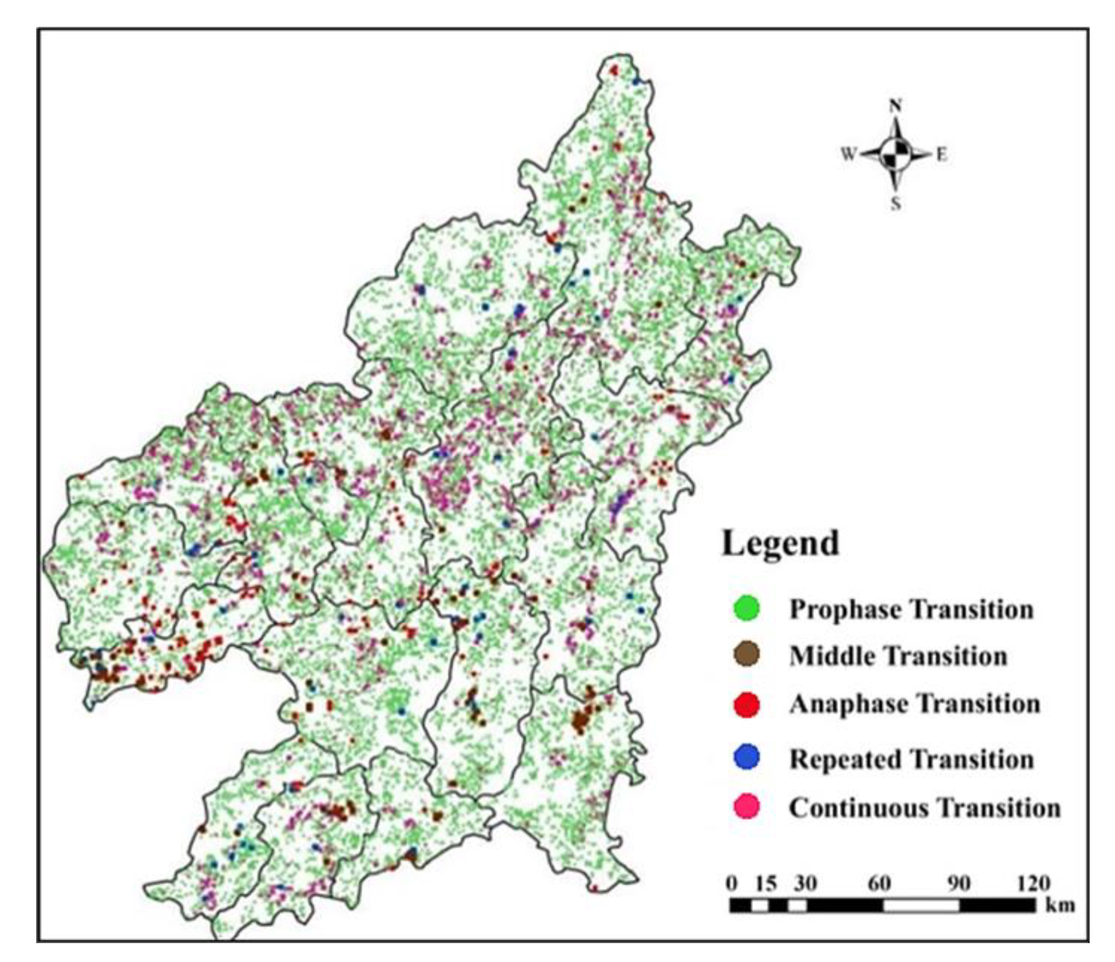
2.3.2. Geo-information Tupu Change Analysis

Geo-information Tupu is an effective method to study land use pattern and evolution [26]. Tupu is based on remote sensing (RS), geographic information system (GIS) and computer mapping, which is capable of uniting the “Tu referring to space unit characteristics” and “Pu referring to the starting point and process of events” as one to reveal the development and change rule of geographic things [27]. Based on the theory of Geo-information Tupu, combined with land use data of six periods and supported by ArcGIS 10.4, to conduct map algebraic operation and build Tupu models for land use change of Gannan region. The calculation formula is [28]

$$\mathrm{T}={\mathrm{Y}}_1\times 10^{\mathrm{n}-1}+{\mathrm{Y}}_2\times 10^{\mathrm{n}-2}+\cdots +{\mathrm{Y}}_{\mathrm{n}}\times 10^{\mathrm{n}-\mathrm{n}}$$

(2)

where T is the Tupu unit code value representing the Tupu model characteristics at the research stage; Y_n is a representation of the code value of the land use unit in a given year; n is the number of land use type. Based on this formula, conducting map algebraic operation can obtain the Tupu of land use change of Gannan process during 1990–2000, 2000–2010, and 2010–2015. In order to further analyze the spatiotemporal characteristics of land transition process, this paper builds classification system of the land transition mode Tupu during 1990–2015 [29].

2.3.3. LCDM Model

The land use change direction model (LCDM) involves a primitively assessment of the impact of land use changes on ecosystem functions [30]. It represents the direction of land use change in the research area. And the analytic hierarchy process (AHP) is used to obtain the weights of each type [31]. Each weight value represents the comprehensive ecological level of land use types, and the ecological levels of different land use types can be referred [31]. The formula is as follows:

$$LCDM= \frac{{{\displaystyle \sum }}_{i=1}^n\left[A_{ij}\times \left(D_j-D_i\right)\right]}{A}\times 100\%$$

(3)

where LCDM refers to the value of land use change, i∈[1,n]; i refers to the i-th land use cover; j reflects j-th land use cover transformed from the i-th land cover; A_ij refers to the value of land use change area from i-th to j-th; Di represents the ecological level [31] of the land use types before the land use cover change. D_j represents the ecological level [31] of the land use types after the land use cover change. A refers to the total conversion area of all land use types throughout the research area during the study period.

2.3.4. Ecosystem Health Assessment

In this paper, we use VORS model to evaluate ecosystem health. Ecosystem health assessment includes four indicators: vigor, organization, resilience and ecosystem services value [13,14,32] (

Table 1. Index system of ecosystem health assessment and data source.

Objective	Indicator	Factor	Data Source
Ecosystem health index (EHI)	Ecosystem vigor (EV)	Vegetation cover index	Land use data of 1990, 1995, 2000, 2005, 2010, and 2015 in Gannan
	Ecosystem organization (EO)	Landscape heterogeneity index
		Landscape connectivity index
		Patch connectivity index
	Ecosystem resilience (ER)	Ecosystem resilience index
	Ecosystem service (ES)	Ecosystem service value

). The ecosystem health index formula is as follows [33]:

$$EHI=\sqrt{PHI\times ESV}$$

(4)

$$PHI=\sqrt[3]{EV\times EO\times ER}$$

(5)

where EHI and PHI respectively represent ecosystem health value and ecosystem physical health status. And EV, EO, ER, and ESV respectively represent ecosystem vigor, ecosystem organization, ecosystem resilience and ecosystem services value. In order to eliminate the different dimensions of the index, EHI, PHI, EV, EO, ER, and ESV are normalized from 0 to 1 [34]. The natural break point method in GIS is used to divide the health level of the ecosystem into five levels: Degraded, Unhealthy, Average Health, Suboptimal Health, and Highest Health.

Natural ecosystem vigor generally indicates the primary productivity, metabolic capacity and activity capacity of the ecosystem [35]. In this paper, vegetation cover index based on land use types is used to express the vigor of ecosystem [36].

Organizational factors represent the structural stability of ecosystem, including spatial heterogeneity, landscape connectivity and landscape morphology [37]. The index equation of ecosystem organization was obtained by referring to relevant literature [19].

The ecosystem resilience value reflects an ecosystem’s ability to maintain its construction and pattern in the face of external disturbances [38]. The sum of the area-weighted ecosystem resilience coefficients of each land use type is used to measure the ecosystem resilience [19]. The calculation formula of ecosystem resilience index was obtained by referring to relevant literature [19].

Based on the measurement model proposed by Costanza (1997) [39] and the value per unit area of ecosystem services in China proposed by Xie et al. (2008) [40], which is an universal way to calculate the value of ecosystem services (ESV). We used Xie’s table to obtain ESV in Gannan during 1990–2015. The calculation formula of ESV is as follows:

$$ESV = {\displaystyle \sum }_{i=1}^n{A}_i \times P_i$$

(6)

where ESV refers to the total ecosystem service values of per unit, A_i refers to the area of land use type i, and P_i refers to the values per unit area of land use type i.

2.3.5. Human Interference Assessment

Hemeroby index quantifies the degree of human interference by considering the level of disturbed landscapes or habitats against natural landscapes or habitats within a study area. The hemeroby index equation refers to previous studies [41], as follows:

$$D=\frac{{{\displaystyle \sum }}_{i=1}^{m}H{I}_i·S_i}{S}$$

(7)

where D represents the human interference degree of a grid, HI_i represents the interference index of i-th landscape type, S_i is the area of i-th landscape type, and S is the total area of grid unit.

2.3.6. Spatial Correlation Analysis between Ecosystem Health and Human Interference

We use spatial correlation analysis to explore the spatial relationship and agglomeration model between ecosystem health and human interference in Gannan. Moran’s I index indicates the spatial correlation proposed by Moran (1950), reflecting the similarity of the spatially adjacent regional unit value. In this study, global bivariate Moran’s I index and local bivariate Moran’s I index in GeoDa spatial analysis software are used to analyze the spatial relationship. Global bivariate Moran’s I is used to explore spatial correlations between ESH and human interference level of Gannan, while local bivariate Moran’s I shows spatial correlations within different spatial units [42]. The formula used are as follows:

$$I=\frac{N{{\displaystyle \sum }}_i^N{{\displaystyle \sum }}_{j\ne i}^N{W}_{ij}{Z}_i{Z}_j}{\left(N-1\right){{\displaystyle \sum }}_i^N{{\displaystyle \sum }}_{j\ne i}^N{W}_{ij}}$$

(8)

$$I_{kl}^i=Z_k^i{{\displaystyle \sum }}_{j=1}^N{W}_{ij}{Z}_l^j$$

(9)

$$Z_k^i=\frac{X_k^i-{\overline{X}}_k}{{\sigma }_k}$$

(10)

$$Z_l^j=\frac{X_l^j-{\overline{X}}_l}{{\sigma }_l}$$

(11)

where $I$ is the global bivariate Moran’s I for ESH and human interference, $I_{kl}^i$ is the local bivariate Moran’s I for ESH and human interference level, $N$ represents the total number of spatial units, $W_{ij}$ is spatial weight matrix for measuring spatial correlation between the i and j spatial unit [43], $Z_i$ is the deviation between the attribute of i spatial unit and the average of attribute, $Z_j$ is the deviation between the attribute of j spatial unit and the average of attribute, $X_k^i$ is the value of attribute k of spatial unit i, ${\overline{X}}_k$ is the average of attribute k, ${\sigma }_k$ is the variance of attribute k, $X_l^j$ is the value of attribute l of spatial unit j, ${\overline{X}}_l$ is the average of attribute l, and ${\sigma }_l$ is the variance of attribute l.

The values of $I$/$I_{kl}^i$ range from −1 to 1. A positive $I$/$I_{kl}^i$ value demonstrates a positive spatial correlation between ESH and human interference, which signifies that a unit with high ESH level is surrounded by units with high interference level. Conversely, a negative $I$/$I_{kl}^i$ indicates a negative spatial correlation, showing that a unit with high ESH level is surrounded by low interference level units. The high absolute value of $I$/$I_{kl}^i$ indicates that the spatial correlation is strong. In this study, we used permutation tests (9999 permutations) to evaluate the statistical significance of bivariate Moran’s I [42]. In order to get credible results, we set the statistically significance value at 0.1% level for spatial correlation between ESH and human interference.

3. Results

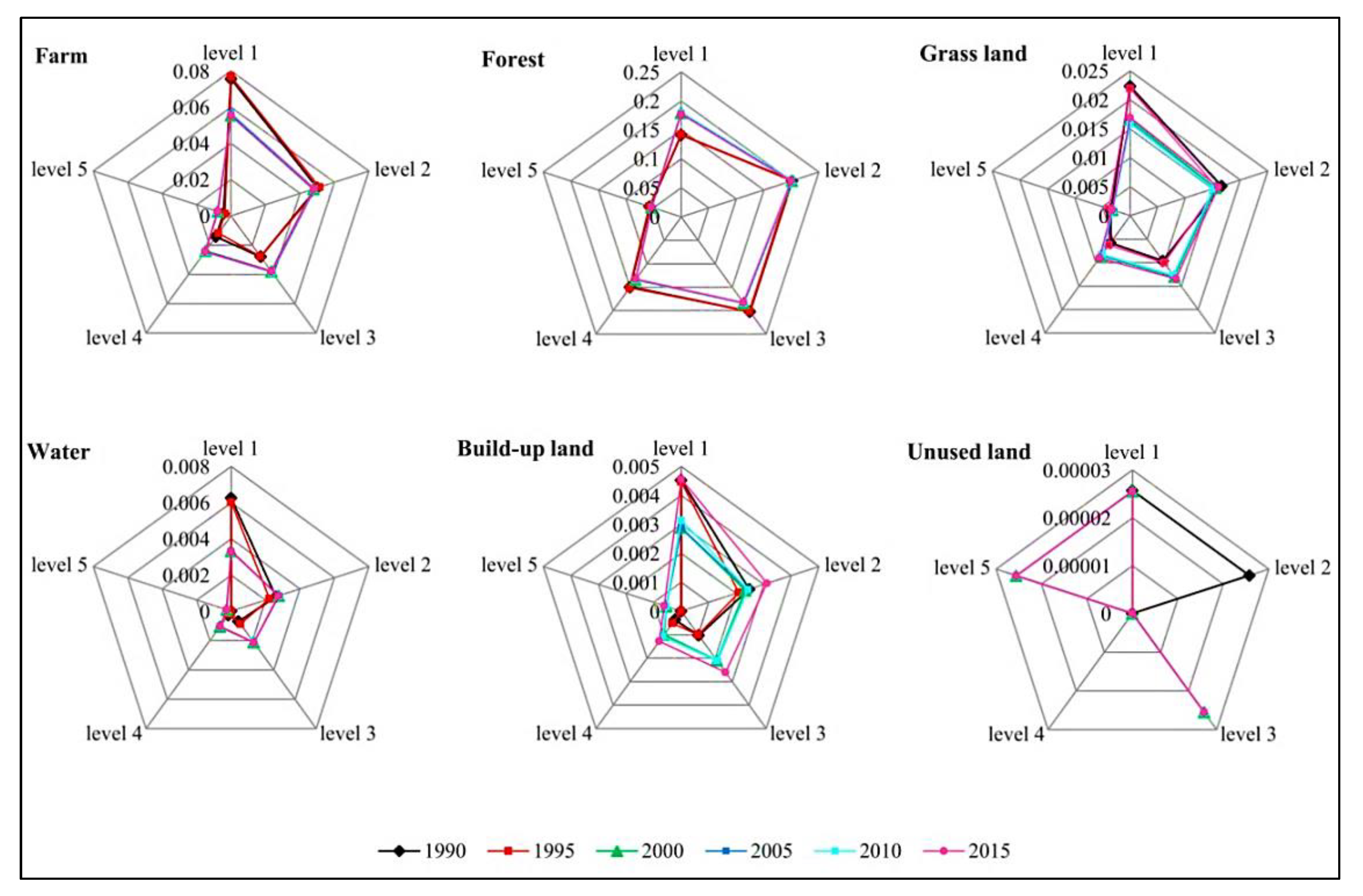
3.1. Temporal–Spatial Variation of Land Use Based on Terrain Gradient

The area proportion of land use types at different terrain gradients are presented in Figure 2. In this study, land types change significantly along the terrain gradient. The area proportion of farm, grassland, water and build-up land gradually decreased with the increase of the terrain gradient during 1990 to 2015. The area of forest reached the maximum on the third terrain gradient, and then gradually decreased during 1990 to 2015. The unused land varied irregularly with the increase of the terrain gradient. The spatial distribution was randomly scattered during 1990 to 2015.

Based on the study of land use change with different terrain gradients, we further analyzed the land use types of conversion in the study area from 1990 to 2015 by using Tupu (Figure 3). The conversion area of farm, forest, and grassland accounted for more than 85% of the whole research area, so the transformation of these three types of land use is representative.

Through the land transition mode Tupu of Gannan during 1990 to 2015 we know that changing the type Tupu unit at a prophase stage (1990–2000) has the largest quantity and area in all types. Most of the forest was converted into farm and grassland at the prophase stage. The area proportion of the middle (2000–2010) and repeated type is the lowest. This indicates that the conversion area of the three land types is relatively small. In addition, the land transition of Anaphase (2010–2015) and the continuous type are mainly concentrated in urban and low terrain gradient areas. Similarly, most of the forest was converted into farm at the Anaphase stage.

To study land use change direction, we calculated the LCDM values of five stages in 1990–2015. The results are as follows: LCDM_1990–1995 = 1.64%, LCDM_1995–2000 = −6.18%, LCDM_2000–2005 = −4.96%, LCDM_2005–2010 = 3.18%, LCDM_2010–2015 = −7.47%. The results of LCDM show that the LULC conversion was beneficial only in 1990–1995 and 2005–2010. However, from 1990 to 2000 and 2000 to 2010, the overall LCDM value of Gannan decreased. Moreover, the most serious period was between 2010 and 2015. In general, from 1990 to 2015, the LCDM value of the whole region gradually decreased. This also indicates that the land use status in Gannan is gradually deteriorating. The corresponding analysis results of land use changing and Tupu are mainly due to the increase of the proportion of farm and building land, and mainly concentrated on the lower terrain gradient. This trend suggests that human activity is increasing at lower terrain gradients.

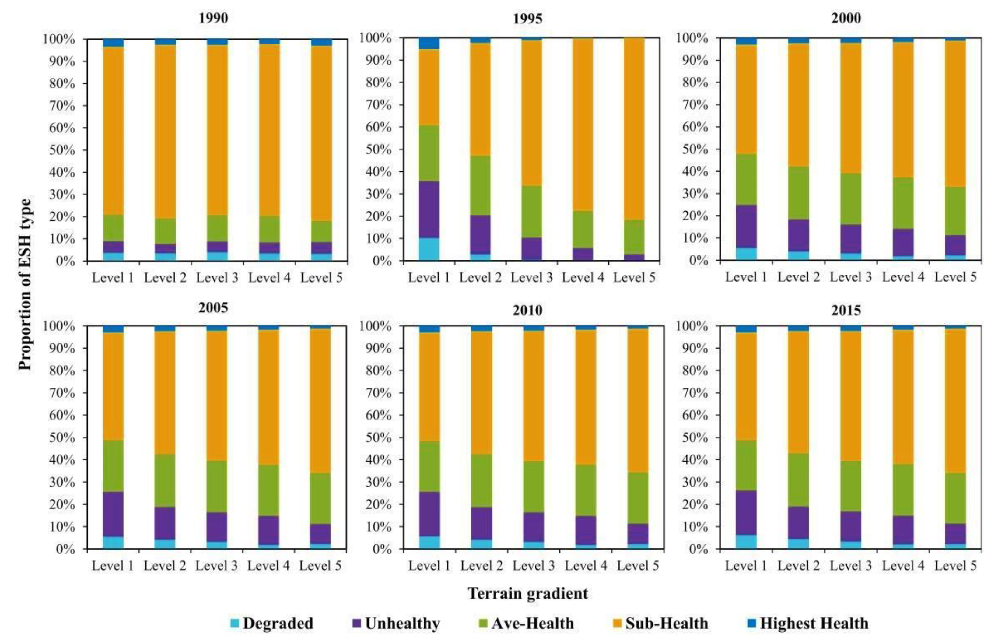
3.2. Assessment of Ecosystem Health

In order to detect the trend of ESH, five levels of ESH were divided based on the Jenks natural break method: highest health, sub-health, average health (ave-health), unhealthy, and degraded. Figure 4 shows the dynamics of the proportion of areas with different ESH levels from 1990 to 2015.

Overall, from 1990 to 2015, an obvious change could be found at different terrain gradients. The areas of unhealthy level and degraded level increased with a decrease in the terrain gradient during the study period. The result is shown in Figure 4.

During 1990 to 2000, the areas with an ave-health level and unhealthy level increased significantly while the areas with a sub-health level decreased, while the areas with a degraded level and the highest health level only experienced little change. During 2000 to 2015, the areas with an unhealthy level increased by 152 km²; the areas with a sub-health level decreased by 260 km². Furthermore, the areas of the highest health level decreased by 8 km².

The results show that the ecosystems of Gannan were in a sub-health level during 1990 to 2015. Compared to 1990, in 2015, the area with the highest health level decreased by 0.48%, while the area with an unhealthy level increased by 10.17%. Moreover, the areas with a degraded level increased by 0.41%. These results suggest that the ecosystem health in Gannan deteriorated from 1990 to 2015.

The changes in different terrain gradient with five ecosystem health levels showed that areas with lower terrain gradients have a relatively weak level of ecosystem health. From 1990 to 2015, the area with a degraded ecosystem health level on the first terrain gradient accounted for 40.52% of the whole region. Additionally, ecosystems in Gannan were healthy in 1990 and then experienced a rapid deterioration from 1995. The proportion of areas with a sub-health level and the highest health level was less than 60% after 1995, with 57.9% in 2015. This result shows that the decrease in an ecosystem health level in a human inhabit district mainly happened between 1995 and 2015, which was related to the rapid urbanization.

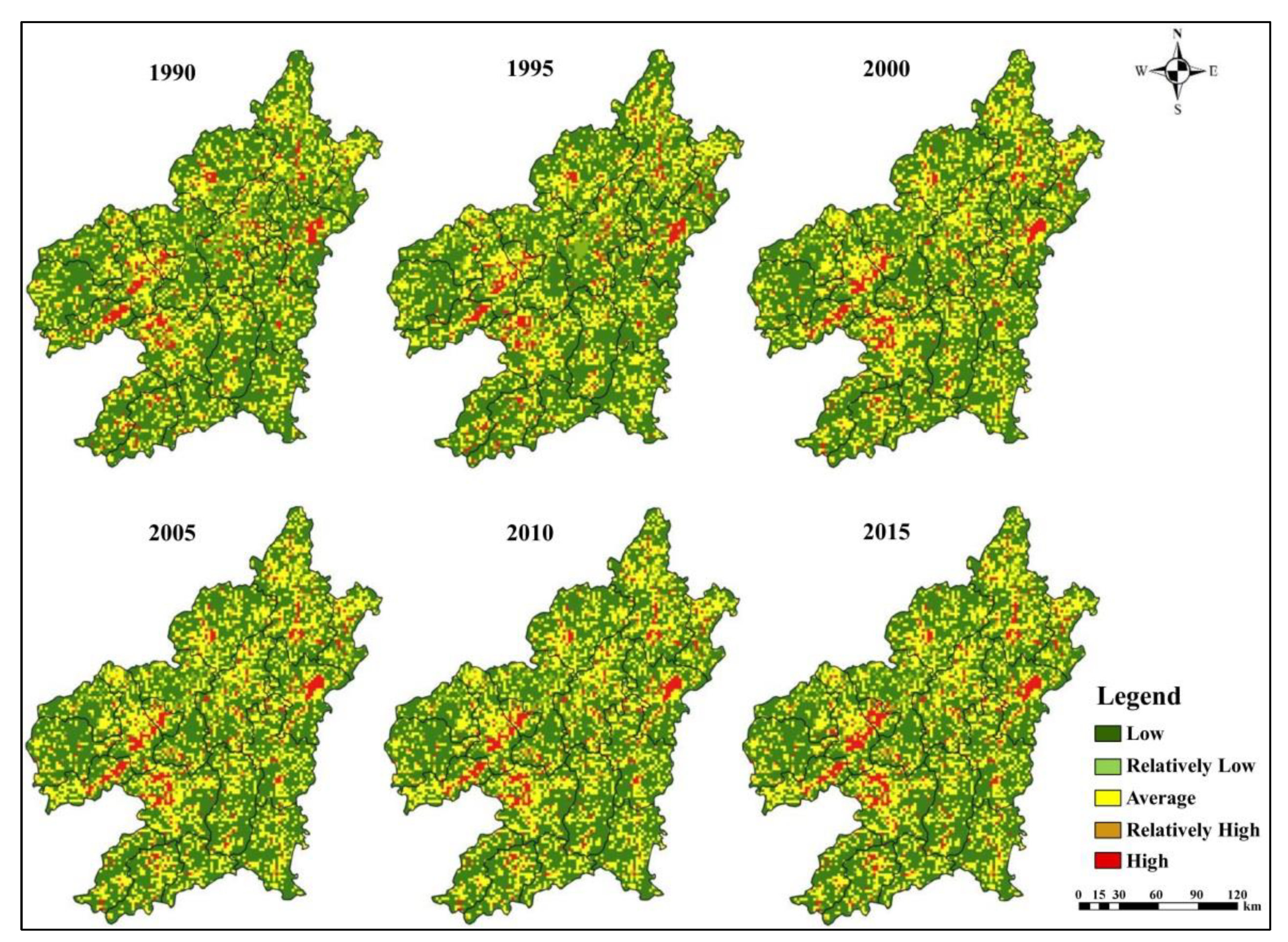
3.3. Ecosystem Health Heterogeneity by Hot Spots Mapping

In order to study spatial heterogeneity of ESH at different terrain gradients, we explored results by performing a Getis-Ord Gi* test to visualize the concentrations of high or low values within the dataset (Figure 5) (

Table 2. Grid number of cold spots and hot spots from 1990 to 2015.

	1990	1995	2000	2005	2010	2015
Cold Spots	990	1146	1155	1151	1148	1136
Hot Spots	374	339	365	365	363	356
Not significant	8648	8527	8492	8496	8501	8520
Total	10,012	10,012	10,012	10,012	10,012	10,012

). Overall, the proportions of the hot spot areas are 0.0374, 0.0339, 0.0365, 0.0365, 0.0362, and 0.0356, respectively, for the six years, showing a declining tendency. The proportions of the cold spot areas are 0.0989, 0.1146, 0.1154, 0.1150, 0.1147, and 0.1129, respectively. Furthermore, the proportions of non-significance spots are 0.8639, 0.8517, 0.8476, 0.8480, 0.8485, and 0.8510, respectively. The result shows that the area with a poor ecosystem health level was expanding and the area with a good health level was decreasing.

From a spatial perspective, there is significant ESH heterogeneity in the study area. After superimposing the distribution map of cold and hot spots with the terrain gradient, we found that almost all the areas where cold spots gather are located on the first and second terrain gradients. On the contrary, hot spots are concentrated in areas with higher terrain gradients. In addition, the distribution of cold spot areas is basically consistent with that of high-population areas. This shows that cold spots are mainly concentrated in cities, such as Ruijin City, Ganzhou City and Nankang City. The distribution of hot spot areas is mainly concentrated in Chongyi County, Shangyou County, and Xingguo County. These areas may have high terrain features, so these areas are not suitable for construction extension.

3.4. The Spatial Distribution of Human Interference in Different Terrain Gradient

To verify the relationship between rapid urbanization and ESH, we detected the spatial patterns of urbanization levels. The values of human interference in the study period were as follows: 0.5845, 0.5842, 0.5848, 0.5856, 0.5856, and 0.5863. The results show that the degree of human interference in the whole study area increased significantly from 1990 to 2015.

The spatial distribution characteristics of the human interference degree were obtained by calculating and interpolating the human interference index by grid (Figure 6) (

Table 3. Grid number table for different degree of human interference from 1990 to 2015.

	1990	1995	2000	2005	2010	2015
Low	5900	5928	5831	5821	5785	5760
Relatively Low	118	109	118	114	112	120
Average	3185	3149	3242	3251	3267	3249
Relatively High	459	483	461	458	475	471
High	350	343	360	368	373	412
Total	10,012	10,012	10,012	10,012	10,012	10,012

). It can be seen that a relatively high interference state and a high interference state are mainly concentrated in cities with a large population. For example, the areas with a high interference are concentrated in Ganzhou City, Nankang City, Ruijin City, Dayu County, Xinfeng County, and Xingguo County. Furthermore, the trend of expansion became even more pronounced after 2000.

The superposition analysis of the high interference area and the terrain gradient map shows that the areas with a high interference primarily cluster on the first and second gradient. The proportion of a high interference grid number on the first and second gradient in the total high interference grid number of the study area from 1990 to 2015 was calculated as follows: 0.8571, 0.8758, 0.6316, 0.6315, 0.6373, and 0.6449. The results show that the high interference region occupies a higher proportion in the lower terrain gradient. This is mainly because the lower terrain gradient has a lower elevation and a smaller slope. The area is more suitable for human development and construction. With the increase of the terrain gradient, the degree of human interference also decreases.

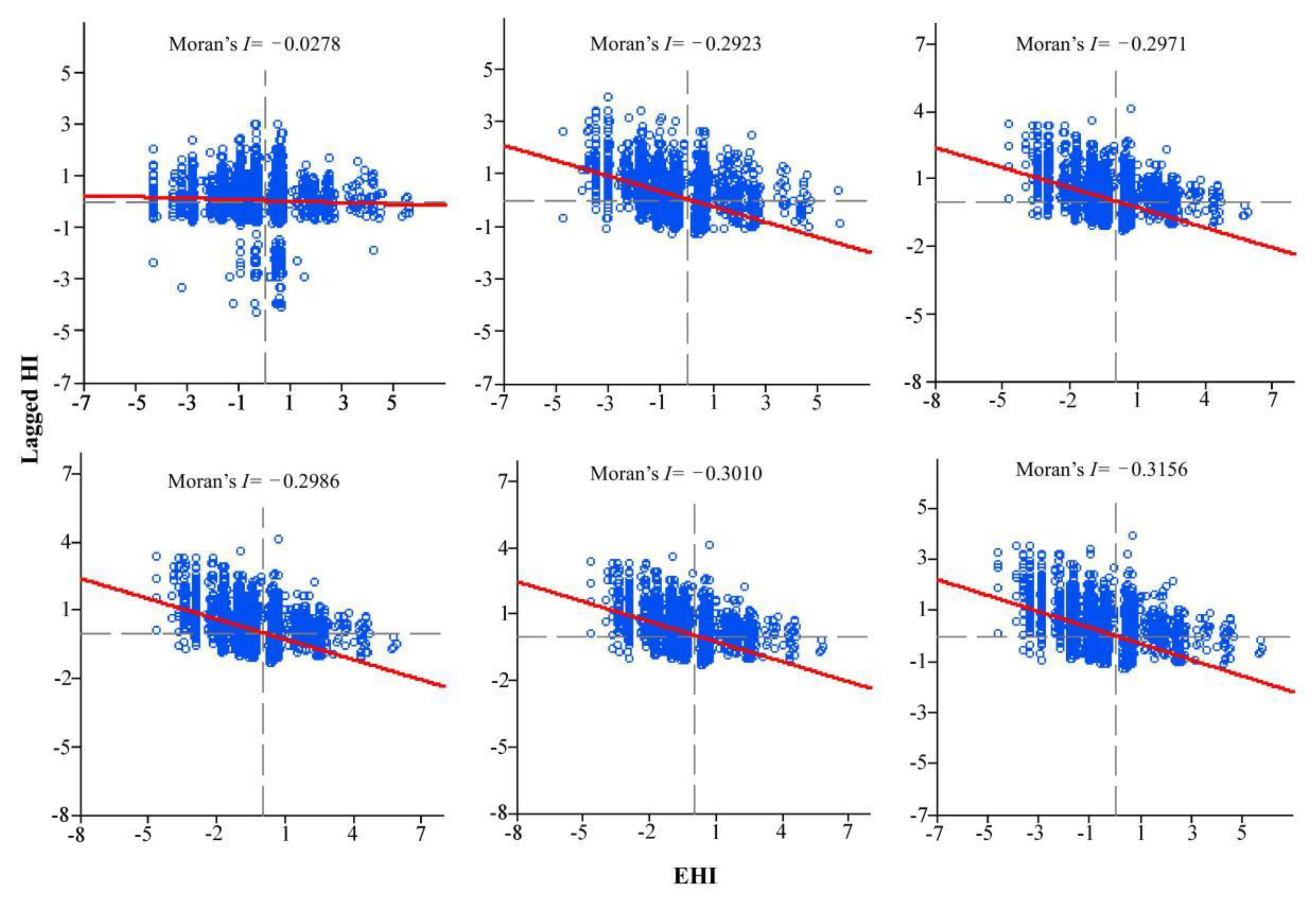
3.5. Spatial Correlation Between ESH and Human Interference in Gannan

In order to further study the spatial response of ecosystem health to human interference in the study area, we conducted spatial global correlation analysis and local correlation analysis for these two variables.

The global spatial correlation between ecosystem health and human interference is shown in

Table 4. Moran’s I Index of ecosystem health (ESH) and human interference and the significant level in Gannan from 1990 to 2015.

Index	1990	1995	2000	2005	2010	2015
I	−0.0278	−0.2923	−0.2971	−0.2986	−0.3010	−0.3156
P	0.0001	0.0001	0.0001	0.0001	0.0001	0.0001
Z	−5.4322	−42.2877	−42.4991	−42.7673	−42.9032	−44.9600

The value I in the table represents Moran’s index; The p-value is the probability, which reflects the probability of an event happening, p < 0.05 indicated a statistical difference, p < 0.01 indicated a statistically significant difference, and p < 0.001 indicated a more statistically significant difference; A z-score is a multiple of the standard deviation that reflects the dispersion or aggregation of the data, |Z| > 2.58, corresponding p < 0.01, indicating a significant statistical difference.

and Figure 7. The global bivariate Moran’s I in Gannan from 1990 to 2015 are −0.0278, −0.2923, −0.2971, −0.2986, −0.3010, and −0.3156. The results indicate that there is a strong negative correlation between ecosystem health and human interference in Gannan, and the Moran’s I index increased significantly from 1990 to 2015. According to Table 1, the null hypothesis is accepted when the absolute value of Z value is greater than 2.58 in the case of 99% confidence. The results of the local spatial correlation analysis are shown in the LISA map (Figure 8). The number of grids with a spatial clustering effect in Gannan accounted for more than 14% under a 95% confidence, and showed a significant upward trend in 25 years. Moreover, the number of Low–High type and High–Low type grids accounts for the largest proportion in the grid with agglomeration effect. Additionally, we found that the effect of Low–High type clustering is more significant at lower terrain gradients. We superimposed the terrain gradient with the Low–High region and found that most of this type aggregate on the first and second gradient. From 1990 to 2015, the number of Low–High grids in Gannan gradually increased, which indicated that the ecosystem health gradually declined with the increase of human interference, and produced a very significant agglomeration effect in space.

Comparing the spatial agglomeration map with the administrative zoning map of Gannan (Figure 1), we found that the Low–High aggregation type is distributed in Ganzhou City, Ruijin City, Nankang City, Dayu County, Huichang County, Xinfeng County, Ningdu County, etc. Among them, the most significant agglomeration effect is located in Nankang City, Dayu County, and Xinfeng County. Additionally, these cities and counties are generally located on the first and second terrain gradient. This trend proves that at lower terrain gradients, the higher the degree of human interference, the worse the health of the ecosystem.

On the contrary, agglomeration effect is of a High–Low type. It is obviously concentrated in Chongyi County and Shangyou County. Consequently, based on the main function zoning of Gannan and the relevant investigation data, we know that Chongyi County belongs to the national key ecological function zone. The ecological environment quality of Chongyi County is splendid with high quality water resources. Moreover, we found that Chongyi County is surrounded by high mountains; hence, the whole area is on higher ground. This leads to a lower degree of human interference, so the topography reduces the external stressors for ecosystem health. Because of its high elevation and slope, this area is not suitable for farming and urban sprawl. Consequently, although Chongyi’s economic development is not the best in the study area, its GDP per capita is among the best. The development mode of Chongyi County is in line with the local actual situation, which not only develops the economic industry but also protects the local environmental resources.

4. Discussion

4.1. Temporal–Spatial Relationship Between ESH and HI

Urban growth has always faced the question of how to balance the relationship between economic development and ecological conservation. For instance, the function of an ecosystem in cities degraded because of urbanization. The regions with a degraded and unhealthy level were all located in areas with a lower terrain gradient. These regions are located in cities or counties with a concentrated population, and the ecological environment problems in these areas are more prominent. For example, various environmental pollution and serious destruction of resources often occur in or around cities with concentrated population [4]. This may be the stress effect of urbanization on the ecological environment as demonstrated by many previous studies [10,11]. With the increase of a terrain gradient, the ecosystem health condition gradually improved. This may be caused by the low degree of human interference in the area with a higher terrain gradient. In higher terrain gradient areas, many production and construction activities are restricted by various geomorphic and climatic conditions. This also reflects the constraint effect of environmental factors on urbanization [11]. As urbanization in the study area is highly dependent on local ecological resources, the contradiction between ecosystem health and human interference is increasing.

This study offers an effective way to understand the impact of urbanization on ESH. From 1990 to 2015, the degree of human interference in the whole region gradually increased, while the health level of the ecosystem gradually decreased. Obviously, the ecosystem health in Gannan is opposite to that of human interference. Moreover, similar previous studies in other areas have come to the conclusion that human interference has a negative impact on ecosystems [44,45]. In addition, the areas with a strong Low–High agglomeration effect were still on the regions with a lower terrain gradient (Figure 8). The result indicates that human interference has a direct negative effect on the ecosystem health in Gannan and has a significant spatial response. However, land use is the most direct way that human interference affects ecosystem health [46]. According to the results of land use change in Gannan, most forest areas and grassland areas were converted to farm land at the highest frequency on the first gradient in 1990–2015. With the rapid urbanization, the increase of building land leads to the loss of more green area, which leads to the continuous deterioration of Gannan’s status. Therefore, scientific land use planning policies involving continuous ESH evaluation and monitoring should be considered by decision makers. However, and this issue is often ignored.

4.2. Spatial Relationship Between ESH and Urbanization for Ecosystem Management

Urban sprawl caused by human activities means a great threat to the health of regional ecosystems and gradually deteriorates ecosystems [47]. In this study, we also obtained the same results. Therefore, how to balance urban development and ecological environment protection is a realistic problem for urban planners and environment managers. Some researches may simply assess the health status of local ecosystems without analyzing the mechanisms of impact and making recommendations [34], for instance, the reasons why ecosystem health is affected in the process of urbanization and the reasons for the spatial heterogeneity of ecosystem health. From this perspective, this study provides some references for the sustainable development of urban growth and the natural environment in Gannan. For example, the higher terrain areas that are rich in forest resources can vigorously develop ecological tourism and continue to protect good ecological resources. In view of the lower terrain areas with a dense population, relevant departments should reduce the exploitation of environmental resources and develop green economy.

The Gannan region is mountainous and hilly, and the terrain condition is also the internal reason for the formation of a ESH pattern. For lower terrain gradient regions, it has a smaller slope and elevation suitable for urban development and construction, so the population is also relatively concentrated. This part of an area has the worst ESH level. For such areas, we suggest a transformation to develop green economy and increase green infrastructure to enhance the supply of ecosystem services [48], instead of blindly pursuing urban expansion and economic development. In addition, these regions should also compare the gap between their own development and that of other prefectures and cities to identify the core issues, so as to achieve precise protection. For urban areas, intensive land development activities should be restricted, which are significant to maintain a sustainable ecosystem. For higher terrain gradient regions, the population distribution is dispersed and the natural ecological environment is in good condition. For such areas, we suggest that appropriate policies should be adopted to prevent a high degree of human interference. For example, regional authorities are actively creating safeguards to prevent major ecological damage and environmental pollution. Such regions with good ecological protection should continue to maintain their development advantages and maintain the awareness of an ecological crisis. In addition, part of the study area can refer to the economic development model of Chongyi County and choose the appropriate economic development path according to the local environmental conditions, so as to realize the balanced development of economic construction and environmental protection.

In this research, the temporal–spatial relationship between ecosystem health and human interference was studied from an original perspective, which provides a database for ecological conservation and ecological management.

5. Conclusions

In this study, we selected multiple indicators to measure ESH at different terrain gradients, and we explored the spatial correlations between urbanization and ESH by heterogeneity and hotspot analysis. Ecosystems are complex and fragile in urban agglomeration, and easily affected by human activities. In view of the impact of urbanization on the ecosystem health in Gannan, government departments are required to conduct reasonable ecological planning according to the actual situation, so as to contribute to the sustainable development of the whole region. In this article, the results showed the following: The urbanization caused by human interference in Gannan indirectly affects ESH by changing land use patterns. Moreover, the ESH and human interference in Gannan had distinct differentiation characteristics on different terrain gradients from 1990 to 2015. In the lower terrain gradient area, urbanization was more serious, the degree of human interference was higher, and the ESH was worse. Through spatial correlation analysis, we know that human interference had a significant negative effect on ESH, and this negative effect gradually increased from 1990 to 2015. In addition, this negative effect was the most significant on the lower terrain gradient according to the LISA map. The results of this study clearly showed the temporal–spatial distribution change law of ESH in Gannan. Therefore, different measures could be taken to change the health status in different terrain gradients according to the actual situation.

References

1. Li, B.; Chen, D.; Wu, S.; Zhou, S.; Wang, T.; Chen, H. Spatio-temporal assessment of urbanization impacts on ecosystem services: Case study of Nanjing City, China. Ecol. Indic. 2016, 71, 416–427. [Google Scholar] [CrossRef]
2. Li, H.; Peng, J.; Yanxu, L. Urbanization impact on landscape patterns in Beijing City, China: A spatial heterogeneity perspective. Ecol. Indic. 2017, 82, 50–60. [Google Scholar] [CrossRef]
3. Qiu, B.; Li, H.; Zhou, M. Vulnerability of ecosystem services provisioning to urbanization: A case of China. Ecol. Indic. 2015, 57, 505–513. [Google Scholar] [CrossRef]
4. Manuel-Navarrete, D.; Gómez, J.J.; Gallopín, G. Syndromes of sustainability of development for assessing the vulnerability of coupled human–environmental systems. The case of hydrometeorological disasters in Central America and the Caribbean. Glob. Environ. Chang. 2007, 17, 207–217. [Google Scholar] [CrossRef]
5. Su, M.; Fath, B.D.; Yang, Z. Urban ecosystem health assessment: A review. Sci. Total Environ. 2010, 408, 2425–2434. [Google Scholar] [CrossRef]
6. Zeng, C.; Deng, X.; Xu, S. An integrated approach for assessing the urban ecosystem health of megacities in China. Cities 2016, 53, 110–119. [Google Scholar] [CrossRef]
7. Brentrup, F.; Küsters, J.; Lammel, J.; Kuhlmann, H. Life cycle impact assessment of land use based on the hemeroby concept. Int. J. Life Cycle Assess. 2002, 7, 339–348. [Google Scholar]
8. Fehrenbach, H.; Grahl, B.; Giegrich, J.; Busch, M. Hemeroby as an impact category indicator for the integration of land use into life cycle (impact) assessment. Int. J. Life Cycle Assess. 2015, 20, 1511–1527. [Google Scholar] [CrossRef]
9. Wu, Y.; Wu, Z. Quantitative assessment of human-induced impacts based on net primary productivity in Guangzhou, China. Environ. Sci. Pollut. Res. Int. 2018, 25, 11384. [Google Scholar] [CrossRef]
10. Fang, C.L.; Liu, H.M.; Li, G.D. International progress and evaluation on interactive coupling effects between urbanization and the eco-environment. J. Geogr. Sci. 2016, 26, 1081–1116. [Google Scholar] [CrossRef]
11. Liu, Y.B.; Li, R.D.; Song, X.F. Correlation analysis between regional urbanization and ecological environment coupling in China. Acta Geogr. Sin. 2005, 2, 237–247. [Google Scholar]
12. Chen, J. Rapid urbanization in China: A real challenge to soil protection and food security. Catena 2007, 69, 1–15. [Google Scholar] [CrossRef]
13. Rapport, D.J. What constitutes ecosystem health? Perspect. Biol. Med. 1989, 33, 120–132. [Google Scholar] [CrossRef]
14. Rapport, D.J. Eco-cultural health, global health, and sustainability. Ecol. Res. 2011, 26, 1039–1049. [Google Scholar] [CrossRef]
15. Kim, Y.O.; Xu, F.L. Marine ecosystem health assessments in Korean coastal waters. Ocean Sci. J. 2014, 49, 249–250. [Google Scholar] [CrossRef] [Green Version]
16. Wu, W.; Xu, Z.X.; Zhan, C.S.; Yin, X.W.; Yu, S.Y. A new framework to evaluate ecosystem health: A case study in the Wei River basin, China. Environ. Monit. Assess. 2015, 187, 460. [Google Scholar] [CrossRef]
17. Wang, X.B.; Liu, W.N.; Wu, W.L. A holistic approach to the development of sustainable agriculture: Application of the ecosystem health model. Int. J. Sustain. Dev. World 2009, 16, 339–345. [Google Scholar] [CrossRef]
18. Styers, D.M.; Chappelka, A.H.; Marzen, L.J.; Somers, G.L. Developing a land-cover classification to select indicators of forest ecosystem health in a rapidly urbanizing landscape. Landsc. Urban Plan. 2010, 94, 158–165. [Google Scholar] [CrossRef]
19. He, J.; Pan, Z.; Liu, D.; Guo, X. Exploring the regional differences of ecosystem health and its driving factors in China. Sci. Total Environ. 2019, 673, 553–564. [Google Scholar] [CrossRef]
20. Meng, Z.Q.; Long, L.B.; She, Q.N.; Cheng, D.Y.; Liu, M. Assessment of ecological conditions over China’s coastal areas based on land use/cover change. J. Appl. Ecol. 2018, 29, 3337–3346. [Google Scholar]
21. Sun, T.; Lin, W.; Chen, G.; Guo, P.; Zeng, Y. Wetland ecosystem health assessment through integrating remote sensing and inventory data with an assessment model for the Hangzhou Bay, China. Sci. Total Environ. 2018, 566, 627–640. [Google Scholar] [CrossRef] [PubMed]
22. Tong, C.; Wu, J.; Yong, S.; Yang, J.; Yong, W. A landscape-scale assessment of steppe degradation in the Xilin River Basin, Inner Mongolia, China. J. Arid Environ. 2004, 59, 133–149. [Google Scholar] [CrossRef]
23. Wang, D.G.; Hu, B.Q.; Rao, Y.X.; Li, W.H. Research on functional zoning of karst land system at county regional scale based on the methods of lattice and ANN. Res. Soil Water Conserv. 2012, 19, 131–136. [Google Scholar]
24. Gong, W.; Wang, H.; Wang, X.; Fan, W.; Stott, P. Effect of terrain on landscape patterns and ecological effects by a gradient-based RS and GIS analysis. J. For. Res. 2017, 28, 1061–1072. [Google Scholar] [CrossRef]
25. Jenks, G.F. The data model concept in statistical mapping. Int. Year Book Cartogr. 1967, 7, 186–190. [Google Scholar]
26. Wang, Z.M.; Zhang, B.; Zhang, S.Q. Estimates of loss in ecosystem service values of Songnen Plain from 1980 to 2000. J. Geogr. Sci. 2005, 15, 82–88. [Google Scholar] [CrossRef]
27. Ye, Q.H.; Liu, G.H.; Lu, Z.; Gong, Z.H. Research of TUPU on land use/land cover change based on GIS. Prog. Geogr. 2002, 21, 349–357. [Google Scholar]
28. Wang, J.L.; Shao, J.A.; Li, Y.B. Geo-spectrum based analysis of crop and forest land use change in the recent 20 years in the three gorges reservoir area. J. Nat. Resour. 2015, 30, 235–247. [Google Scholar]
29. Lu, X.; Shi, Y.Y.; Huang, X.J.; Sun, X.F.; Miao, Z.W. Geo-spectrum characteristics of land use change in Jiangsu Province, China. Chin. J. Appl. Ecol. 2016, 27, 1077–1084. [Google Scholar]
30. Zubaida, M.B.; Xia, J.X.; Polat, M.; Shi, Q.D.; Zhang, R. Spatiotemporal changes of land use/cover from 1995 to 2015 in an oasis in the middle reaches of the Keriya River, southern Tarim Basin, Northwest China. Catena 2018, 171, 416–425. [Google Scholar]
31. Tayfun, T.; Mevlut, U. Evaluation of reallocation criteria in land consolidation studies using the analytic hierarchy process (AHP). Land Use Policy 2013, 30, 541–548. [Google Scholar]
32. Costanza, R.; Norton, B.G.; Haskell, B.D. Ecosystem Health: New Goals for Environmental Management; Island Press: Washington, DC, USA, 1992. [Google Scholar]
33. Kang, P.; Chen, W.; Hou, Y.; Li, Y. Linking ecosystem services and ecosystem health to ecological risk assessment: A case study of the Beijing-Tianjin-Hebei urban agglomeration. Sci. Total Environ. 2018, 636, 1442–1454. [Google Scholar] [CrossRef] [PubMed]
34. Liu, D.; Hao, S. Ecosystem health assessment county-scale using the pressure-state-response framework on the loess plateau, China. Int. J. Environ. Res. Public Health 2016, 14, 2. [Google Scholar] [CrossRef] [PubMed] [Green Version]
35. Phillips, L.B.; Hansen, A.J.; Flather, C.H. Evaluating the species energy relationship with the newest measures of ecosystem energy: NDVI versus MODIS primary production. Remote Sens. Environ. 2008, 112, 3538–3549. [Google Scholar] [CrossRef]
36. Cui, E.; Ren, L.; Sun, H. Evaluation of variations and affecting factors of eco-environmental quality during urbanization. Environ. Sci. Pollut. Res. Int. 2015, 22, 3958. [Google Scholar] [CrossRef] [PubMed]
37. Xiao, R.; Liu, Y.; Fei, X.; Yu, W.; Zhang, Z.; Meng, Q. Ecosystem health assessment: A comprehensive and detailed analysis of the case study in coastal metropolitan region, Eastern China. Ecol. Indic. 2019, 98, 363–376. [Google Scholar] [CrossRef]
38. Costanza, R. Ecosystem health and ecological engineering. Ecol. Eng. 2012, 45, 24–29. [Google Scholar] [CrossRef] [Green Version]
39. Costanza, R.; D’Arge, R.; De Groot, R.; Farber, S.; Grasso, M.; Hannon, B.; Limburg, K.; Naeem, S.; O’Neill, R.V.; Paruelo, J. The value of the world’s ecosystem services and natural capital. Nature 1997, 387, 253–260. [Google Scholar] [CrossRef]
40. Xie, G.D.; Zhen, L.; Lu, C.X.; Xiao, Y.; Chen, C. Expert knowledge based valuation method of ecosystem services in China. J. Nat. Resour. 2008, 23, 911–919. [Google Scholar]
41. Chen, A.; Zhu, B.; Chen, L.; Wu, Y.; Sun, R. Dynamic changes of landscape pattern and eco-disturbance degree in Shuangtai estuary wet land of Liaoning Province, China. Chin. J. Appl. Ecol. 2010, 21, 1120–1128. [Google Scholar]
42. Anselin, L. Local indicators of spatial analysis—LISA. Geogr. Anal. 1995, 27, 93–115. [Google Scholar] [CrossRef]
43. Amaral, P.V.; Anselin, L. Finite sample properties of Moran’s—Test for spatial autocorrelation in Tobit models. Pap. Reg. Sci. 2014, 93, 773–781. [Google Scholar] [CrossRef]
44. Liang, L.; Chen, F.; Shi, L. NDVI-derived forest area change and its driving factors in China. PLoS ONE 2018, 13, e0205885. [Google Scholar] [CrossRef] [PubMed]
45. Wang, S.; Ma, H.; Zhao, Y. Exploring the relationship between urbanization and the eco-environment—A case study of Beijing-Tianjin-Hebei region. Ecol. Indic. 2014, 45, 171–183. [Google Scholar] [CrossRef]
46. Mitchell, M.G.E.; Suarez-Castro, A.F.; Martinez-Harms, M. Reframing landscape fragmentation’s effects on ecosystem services. Trends Ecol. Evol. 2015, 30, 190–198. [Google Scholar] [CrossRef] [Green Version]
47. Gordon, A.; Simondson, D.; White, M. Integrating conservation planning and land use planning in urban landscapes. Landsc. Urban Plan. 2009, 91, 183–194. [Google Scholar] [CrossRef]
48. Wang, J. Environmental costs: Revive china’s green GDP programme. Nature 2016, 534, 37. [Google Scholar] [CrossRef]
Figure 1. Location of the study area.
Sustainability 12 01773 g001
Figure 2. Proportion of land use area in Gannan region on the basis of terrain gradients. Level 1–5 represents five terrain gradients. Except for unused land, trends for all years (1990–2015) in the remaining land use types are shown on five gradients. The variation trend of farm from 2000 to 2015 was similar, which caused the overlap between the lines. Unused land had no value on all gradients in 1995, and had values on gradient 1, 3, and 5 in 2000–2015.
Sustainability 12 01773 g002
Figure 3. Pattern Tupu of three land use types change during 1990–2015 in Gannan.
Sustainability 12 01773 g003
Figure 4. Changes of ecosystem health in Gannan based on temporal and terrain gradients.
Sustainability 12 01773 g004
Figure 5. Distribution of hotspots for ecosystem health in Gannan from 1990 to 2015.
Sustainability 12 01773 g005
Figure 6. Spatial distribution of human interference in Gannan from 1990 to 2015.
Sustainability 12 01773 g006
Figure 7. Moran’s I Index of ecosystem health index (EHI) and human interference (HI) in Gannan from 1990 to 2015.
Sustainability 12 01773 g007
Figure 8. Spatial aggregation of ESH and human interference in Gannna from 1990 to 2015.
Sustainability 12 01773 g008