Global Sensitivity Analysis of the Standardized Precipitation Evapotranspiration Index at Different Time Scales in Jilin Province, China

Abstract

The Standardized Precipitation Evapotranspiration Index (SPEI) has been widely applied, due to its multi-scalar features and the ability to identify different drought types. However, its sensitivity to climatic variables still remains unclear, especially at different time scales. Therefore, this study investigates the sensitivity of SPEI to average temperature (T_mean), diurnal temperature ranges (T_delta), relative humidity (RH), solar radiation (Rs), wind speed (U₂), geothermal flux (G), and precipitation (P) from 1957 to 2017 using the extended Fourier Amplitude Sensitivity Test at different time scales in Jilin Province, China. Jilin Province experienced a significant rise in T_mean, and a sharp decrease in T_delta, Rs, and U₂. P is undoubtedly the most influential factor to the SPEI among the meteorological variables, which explained 59.9%–97.9% of the total variability, especially during the main crop growing season (from May to September). While T_mean, RH, or U₂ observably affect the SPEI and cannot be neglected during the nongrowing season. In terms of spatial distribution, the SPEI was mainly affected by P in the eastern region, while it was also influenced by T_mean, RH, and U₂ as well in the western region. The sensitivity of the SPEI differs in time scales: P > T_mean > RH > U₂ > Rs > G > T_delta (1 to 6 month), P > U₂ > RH ≈ T_mean > G > Rs > T_delta (7 to 18 month), and P > U₂ > G > T_mean > RH > Rs > T_delta (more than 24 month time scale), respectively. The results have the potential to provide a reference for agricultural production and management in Jilin Province, China.

1. Introduction

Increasing global temperatures are associated with a rise in the frequency and intensity of extreme weather events, including severe drought and high temperatures [1], particularly in Eurasia [2,3,4] and Africa [5,6]. This has resulted in regional drought research becoming more intricate. In order to accurately monitor drought, scholars and government departments around the world have proposed a series of drought indicators, including the Chinese Z Index (CZI), the Palmer Drought Severity Index (PDSI), the Water Stress Index (WSI) and the Standardized Precipitation Index (SPI). Among them, the widely used SPI is simple to calculate, flexible, and effective. However, indices such as the SPI and CZI fail to account for evapotranspiration. Moreover, recent studies have demonstrated that the increased evapotranspiration caused by rising temperature cannot be ignored [7,8]. Thus, the use of more comprehensive indicators is becoming more popular. In particular, the SPEI, put forward by Vicente-Serrano et al. (2010), is not only highly sensitive to changes in evaporation, but is also characterized by a simple calculation and its ability to consider multiple time scales. Due to a broad range of meteorological variables in the context of global warming, the SPEI is able to comprehensively identify different drought types [7,9,10,11,12]. Thus, the SPEI has proved to be highly effective in the detection, monitoring, and exploration of drought [7].

Numerous studies have applied the SPEI in order to evaluate drought characteristics and atmospheric drought mechanisms, and to perform drought assessments and monitoring [9,13,14,15,16,17,18]. For example, Chen et al. [8] used the SPI and SPEI to analyze the characteristics of drought occurrence in Liaoning Province from 1960 to 2015. They determined that the SPEI was able to better explain yield variation in major cereal crops (39%–78%) due to its accounting of P and reference evapotranspiration (ET_o). Peña-Gallardo et al. [19] quantified drought using the SPEI and observed that inter-annual changes in crop yields were strongly correlated to drought time scales. Over the past 50 years, empirical models have been developed to estimate ET_o based on different combinations of climatic variables, an important parameter also used for the SPEI calculation, such as the Hargreaves [20], the Priestley–Taylor [21], and the FAO-56 Penman–Montieth (PM) [22] methods. Among these, the FAO-56 PM method was identified as superior for the SPEI calculation [23,24,25,26], due to its ability to accurately estimate drought trends [8].

Sensitivity analysis is effective in the identification of the dominant mechanisms in model behavior [27] and any relationship between variables [28]. It is able to analyze the main role of meteorological variables in regional ET_o assessments [29]. Thus, sensitivity analysis of drought indices to meteorological variables can be applied to analyze the relationship between meteorological variables and drought events [30]. In recent years, the PM equation has been widely used in the sensitivity analysis of ET_o [31,32,33]. Yao et al. [34] observed distinct sensitivities of P and reference evapotranspiration (ET_o) to the SPEI in Xinjiang, and drought condition was mainly determined by the ET_o in the arid zone. Vicente-Serrano et al. [35] also pointed out that precipitation and ET_o had the same sensitivity to SPEI. Despite the large amount of research on the SPEI [36,37], the contribution of each meteorological variable to SPEI fluctuations, as well as the sensitivity of the SPEI to meteorological variables, still remain unclear.

In order to provide a more in-depth investigation of meteorological variable sensitivities to the SPEI, this study applied the Extended Fourier Amplitude Sensitivity Test (EFAST) method [38] to analyze the SPEI global sensitivity. More specifically, T_mean, T_delta, RH, Rs, U₂, G, and P at different time scales were used as the independent variables, and the SPEI was used as the dependent variables. The objectives of this study are to (a) identify the existence of a possible tendency of each of the climatic variables; (b) explore the sensitivity of SPEI to T_mean, T_delta, RH, Rs, U₂, G, and P; and (c) identify the response of the sensitivity of the SPEI to time scales.

2. Materials and Methods

2.1. Description of Study Site

Jilin Province (121°38′–131°19′ E, 40°50′–46°19′ N) is located in the central part of northeast China, with a total area of 187,4000 km² (Figure 1). It exhibits a high altitude in the southeast and low altitude in the northwest. Jilin Province can be divided into two regions: the mountainous terrain in the east and plains in the mid-west [39]. The province has an annual T_mean within the range of 2–6 °C, and a frost-free period for approximately 100–160 d. Mean annual P are higher in the mountains and lower in the western plains, with the average annual P of the whole province being 400–600 mm, more than 80% of which is received in summer.

2.2. Meteorological Data

Meteorological data were collected from the China surface climate data daily dataset (V3.0) released by the National Meteorological Information Center of China (http://data.cma.cn/). The surface climate data daily dataset covering 28 meteorological stations (Figure 1) includes daily precipitation, air temperature (maximum, minimum, and average), atmospheric pressure, relative humidity, wind speed at 10 m above ground, and sunshine hours in Jilin Province from 1957 to 2017. The Inverse Distance Weighted (IDW) method was used to interpolate the daily meteorological data to account for any gaps in the dataset. In addition, the homogeneity and reliability of the meteorological data were tested and controlled by adopting the method described by Liu et al. [40].

2.3. Reference Evapotranspiration

The Penman–Monteith reference evapotranspiration method was selected to estimate seasonal ET_o on the basis of monthly interval in this study:

$$E{T}_{\mathrm{o}}=\frac{0.408\Delta \left(R_n-G\right)+\gamma \frac{900}{T+273}{W}_s\left(e_s-e_a\right)}{\Delta +\gamma \left(1+0.34W_s\right)}$$

(1)

where ET_o is monthly average daily reference evapotranspiration, mm d⁻¹; T is monthly average daily temperature, °C; G is monthly soil heat flux, MJ m⁻² d⁻¹; R_n is the monthly average daily net radiation, MJ m⁻² d⁻¹, computed from actual duration of daily sunshine hours; γ is the psychrometric constant, kPa °C⁻¹; e_s is monthly average of the daily mean saturation vapor pressure (kPa), e_a is monthly average of the daily actual vapor pressure (kPa), $\Delta$ is the slope of saturation vapor pressure curve, kPa °C⁻¹; and w_s is monthly average daily wind speed at height 2 m, m s⁻¹.

Since daily maximum and minimum air temperature are often correlated, the average daily temperature and diurnal temperature ranges are calculated by averaging the mean of the daily maximum and minimum temperature, the difference of the daily maximum and minimum temperature, respectively [41]. The monthly or other time-scale accumulative climatic variables, P and Rs, were estimated by summing the daily data, while the monthly or other timescale mean climatic variables, T_mean, T_delta, RH, and U₂, were estimated by averaging the daily data. When assuming a constant soil heat capacity of 2.1 MJ m⁻³ °C⁻¹ and an appropriate soil depth of 2 m, the soil heat flux at different time periods G can be approximated as [22]:

$$G=2.1\times \frac{T_i-T_{i-1}}{30.5\times m}\times 2=\frac{0.138(T_i-T_{i-1})}{m}$$

(2)

where T_i and T_i−1 is the monthly or other timescale mean temperature (°C) at time i, i − 1; m is the number of months within a specific time scale.

2.4. Trend Analysis

The Mann–Kendall method (MK) [42] was adopted for the detection of trends for the climatic variables. Prior to this, the trend-free prewhitening method was applied in order to eliminate the autocorrelation of data sequences [43]. Following the MK test, the Theil–Sen method [40,44] was used to calculate the magnitude of trends. The MK trend test and Theil–Sen estimator were both implemented by the R package RKT [45].

2.5. Standardized Precipitation Evapotranspiration Index (SPEI)

The SPEI was proposed by Vicente-Serrano et al. [7] for identifying drought episodes. The SPEI was computed using the difference between P and ET_o as the water surplus/deficit indicator. The calculation procedures for the SPEI are as follows:

(1) The water surplus/deficit equation

$$D_i=P_i-E{T}_{\mathrm{o}i}$$

(3)

where $P_i$ is monthly precipitation, ET_oi is potential evapotranspiration and $D_i$ is water surplus/deficit at month i.

(2) log-logistic distribution

Assuming a three-parameter log-logistic distribution, the probability density function of D_i was calculated by the following equation:

$$f\left(x\right)=\frac{\beta }{\alpha }{\left(\frac{x-\gamma }{\alpha }\right)}^{\beta -1}{\left[1+{\left(\frac{x-\gamma }{\alpha }\right)}^{\beta }\right]}^{-2}$$

(4)

while the cumulative probability density function was determined as follows:

$$F\left(x\right)={\left[1+{\left(\frac{\alpha }{x-\gamma }\right)}^{\beta }\right]}^{-1}$$

(5)

where α, β, and γ are the shape, scale, and position parameters, respectively.

(3) The SPEI index series was subsequently derived from the fitted values through the transform of the standardized normal distribution. The equation used for the calculation is as follows:

$$SPEI=W-\frac{C_0+C_{1}W+C_2{W}^2}{1+d_{1}W+d_2{W}^2+d_3{W}^3}$$

(6)

where $W=\sqrt{-2\ln (P)}$ and $P$ is the probability of exceeding a determination value of D. In particular, for p ≤ 0.5, and p = 1 − F(x), while for p > 0.5, P = 1 − P and the sign of the SPEI is reversed. The variables C₀, C₁, C₂, d₁, d₂, and d₃ are constants. A detailed description of the calculation method can be found in [7,46], whereby the specific values of C₀ = 2.515517, C₁ = 0.802853, C₂ = 0.010328, d₁ = 1.432788, d₂ = 0.189269, and d₃ = 0.001308 can be derived.

2.6. Extended Fourier Amplitude Sensitivity Test (EFAST)

The theory of global sensitivity analysis (GSA) was initially proposed by Cukier et al. [47,48,49]. All GSA variables change simultaneously within the value ranges. Hence, the GSA always identify not only the impact of each variable on the variance of the response variable, but the interaction effects of all variables. It can also overcome the shortcomings of local sensitivity analysis, such as calculating one variable at a time, analyzing the change of one variable while maintaining other variables constant, and the lack of interaction effect analysis [50,51]. Numerous GSA methods have been applied in the literature, such as the Extended Fourier Amplitude Sensitivity Analysis (EFAST) [50], the Sobol method [52], and the Morris method [53]. In particular, EFAST is one of the most powerful techniques, and has been recommended by many scholars [38,50]. The underlying method of EFAST global sensitivity analysis is to allow for the input variables of the model to oscillate at different frequencies. In addition, EFAST is able to assess the importance of each variable by evaluating the Fourier coefficients of the model outputs. The basic theory can be described as follows:

Define $y=f\left(x_1,x_2,\dots ,x_k\right)$, and variable X as the k-dimensional space of input variable,

$${\mathsf{\Omega }}^k=\left(x|0\le x_i\le 1\right); i=1,2,\cdots ,k$$

(7)

whereby y is converted to y = f(s) by variable function $G_i(i=1,2,\dots ,k)$, $f(s)=f(G_{\mathrm{1}}(s),G_{\mathrm{2}}(s),\dots ,G_k(s))$. then $x_i=G_i(\sin ({\omega }_{i}s+{\phi }_i)),{\forall }_i=1,2,\dots ,k$. Here, s is the scale variable, ω_i is the frequency variable associated with variable x_i and G_i is the transform function. Assume that φ_i is a phase-shift chosen uniformly within the range [0, 2π], which allows for a change in the starting point of the scheme. Then we have

$$G_i\left(Z\right)=F_i^{-1}\left(\frac{1}{\pi } arcsin\left(Z\right)+\frac{1}{2}\right)$$

(8)

Based on Lu and Mohanty [54], the variable function takes the form, where $F_i^{-1}$ is the inverse cumulative distribution function of the probability distribution function of X_i. Thus the values of x_i are computed as follows:

$$x_i=F_i^{-1}\left(\frac{1}{\pi }arcsin(sin({\omega }_{i}s+{\phi }_i))+\frac{1}{2}\right), x_i={\forall }_i=1,2,\dots ,k$$

(9)

where ${\forall }_i$ is the partial variance generated by the interaction of all orders between X and other variables φ_i, F⁻¹(P) = a + p(b − a) is evenly distributed in [a, b], and $0 < \mathrm{P} < 1$. Variable $x_i$ oscillates periodically at a frequency of ${\omega }_i$, function f is the periodic function of s, with the period of s taken as less than 2π. Following this, f can be expanded into a Fourier series in the integer frequency domain as follows:

$$f\left(x\right)=\sum _{l=-\infty }^{+\infty }\left(A_l\cos \left(ls\right)+B_l\sin \left(ls\right)\right)$$

(10)

where $A_l$ and $B_l$ are Fourier coefficients defined as:

$$\begin{array}{l}{A}_l=\frac{1}{2\pi }\underset{-\pi }{\overset{\pi }{\int }}f\left(s\right)\cos \left(ls\right)ds\\ B_l=\frac{1}{2\pi }\underset{-\pi }{\overset{\pi }{\int }}f\left(s\right)\sin \left(ls\right)ds\end{array}$$

(11)

The spectrum of the Fourier series expansion is defined as ${\mathsf{\Lambda }}_l=A_l^2+B_l^2$, which represents the amplitude of f. The total variance $Var\left(Y\right)$ can be expressed as the sum of the Fourier spectrum elements of f:

$$Var\left(Y\right)=2\sum _{l=1}^{+\infty }{\mathsf{\Lambda }}_l$$

(12)

The partial variance of Y attributed to the main effect of X_i is thus obtained by:

$$V_i=2\sum _{p=1}^{+\infty }{\wedge }_{P{\omega }_i}$$

(13)

In practice the infinite summation is not convenient. The main influence of X_i can be approximated, as described by Mesgouez et al. [50], as follows:

$${\stackrel{⌢}{V}}_i=2{\displaystyle \sum _{P=1}^M{\wedge }_{P{\omega }_{\mathrm{i}}}}$$

(14)

where M is denoted as the interference factor and is generally chosen within the range of [4,6]. Xu and Gertner [55] denoted the total effect of X_i as the maximum value of ${\omega }_{\mathrm{i}}$. In addition, $Var(E\left(Y|X~i\right),$ the sum of the partial variances, is calculated by taking the sum of the frequency spectrum elements for all frequencies between 1 and $M\max \left(\omega ~i\right)$. Note that we assume that the interaction effects ${\omega }_i$ are negligible at these frequencies. The total and partial variances of Y attributed to the total effect of $X_i$ are thus obtained as follows:

$$\widehat{V} =2\sum _{l=1}^{M{\omega }_i}{\wedge }_l$$

(15)

$$\widehat{\mathrm{VT}}=2\sum _{l=1}^{M{\omega }_i}{\wedge }_l-2\sum _{l=1}^{M max\left({\omega }_{~i}\right)}{\wedge }_l=2\sum _{l=M max\left({\omega }_{~i}\right)}^{M{\omega }_i}{\wedge }_l$$

(16)

However, improved results can be obtained by using $N=2M{\omega }_i+1$, $N=4M{\omega }_i+1$ [38]. In general, the effective simulation of partial variance is a function of the interference factor M and the frequency set ${\omega }_{~i}$. In this study, the R package “sensitivity” available on the comprehensive r archive network (CRAN) was used [56].

3. Results

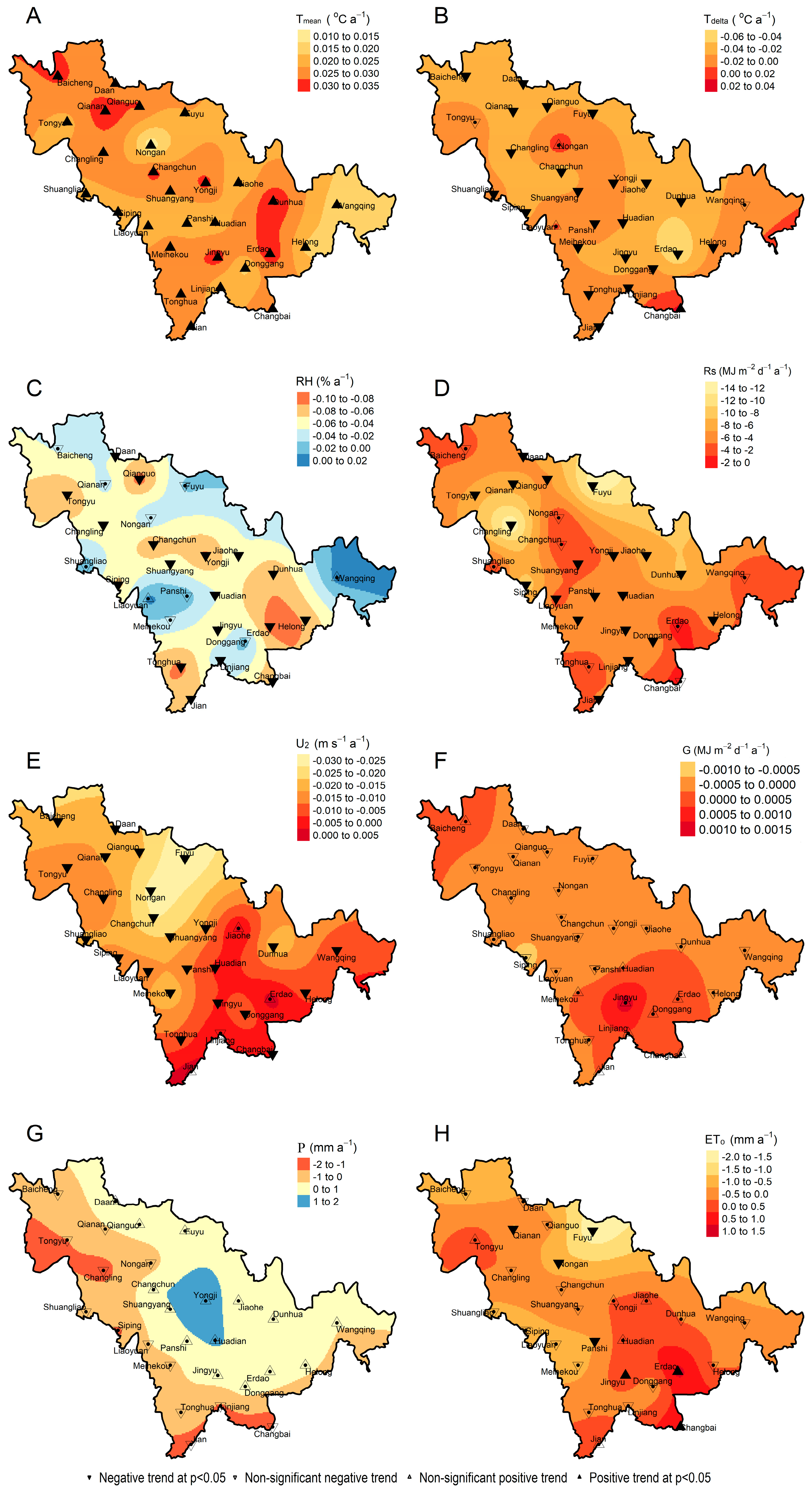
3.1. Meteorological Variable Trend Analysis

Figure 2 presents the spatial distribution of the trend of meteorological variables in Jilin Province, China, over the past 60 years, including T_mean, T_delta, RH, Rs, U₂, G, and P. The Mann–Kendall test demonstrated that T_mean, T_delta, RH, Rs, U₂, and ET_o each exhibited a significant change (p < 0.05) over the past 60 years. Fluctuations were observed for annual P and G, although there was no significant trend detected (p < 0.05).

The T_mean in Jilin Province showed a significant increase (p < 0.05) over the study period (Figure 2A), which is consistent with the global warming general trend. In particular, the maximum increase in T_mean was observed at Dunhua station (0.35 °C/10 a), and the minimum at Nong’an station (0.11 °C (10a)⁻¹). The average increasing rate of T_mean was 0.26 °C (10a)⁻¹, indicating that T_mean increased by 1.56 °C during the past 60 years in Jilin Province, China. Despite the rise in mean temperature, T_delta declined (Figure 2B). The T_delta in 89% of the stations demonstrated a decreasing trend, of which 82% was significant (p < 0.05), as shown in Figure 2B. Averaging the selected 28 stations, T_delta decreases at the rate of 0.19 °C (10a)⁻¹, and decreased by 1.15 °C over the past 60 years. The only three exhibiting an upward trend were at Changbai (significant increase), Liaoyuan, and Nong’an. These results indicate that the T_mean significantly increases over the study period in Jilin Province, while the increases in maximum and minimum temperature are not synchronized, showing a significant negative trend in T_delta.

The RH in Jilin Province generally showed a downward trend, with a mean tendency rate of −0.47% (10a)⁻¹. Among the 28 meteorological stations, 26 stations exhibited a decreasing trend in the RH, and 69.2% of the stations significantly decreased (p < 0.05). Spatially, the maximum positive trend in RH trend (0.08% (10a)⁻¹) was witnessed in Wangqing station in eastern Jilin, and the lowest negative trend was detected in Qiangguo (−0.92% (10a)⁻¹) (Figure 2C). The annual Rs and average U₂ generally demonstrated a significant downward trend, with the mean tendency rate being −52.1 MJ m⁻² d⁻¹ (10a)⁻¹ and −0.12 m s⁻¹ (10a)⁻¹, respectively (Figure 2D,E). The Rs and U₂ decreased by 313 MJ m⁻² d⁻¹ (10a)⁻¹ and 0.72 m s⁻¹ (10a)⁻¹, respectively, over the past 60 years. Among the selected 28 meteorological sites, both Rs in 100% of the stations and U₂ in 89.3% of the stations showed a province-wide decreasing trend, which was consistent with the findings of Wang et al. [57]. This trend was significant at 71.4% of the stations for Rs and 96.0% for U₂, respectively (p < 0.05). The U₂ exhibited an evident spatial variation tend, with a decreasing trend observed from the southeast to northwest. The maximum positive trend reached 0.03 m s⁻¹ (10a)⁻¹ at Erdao station in southeast Jilin, while the minimum negative trend (−0.30 m s⁻¹ (10a)⁻¹) was observed at Fuyu station. Changes in G and annual precipitation over the past 60 years were relatively small compared to those of annual Rs and average U₂ (Figure 2F,G). Though the G of most stations (67.9%) exhibited a downward trend and the annual precipitation of 53.6% of the stations showed an upward trend, but the changes were not significant at the p < 0.05 significant level.

There was a clear spatial distributing in the trend in the ET_o (Figure 2H). In particular, the ET_o observed in southeast Jilin exhibited an upward trend (e.g., 12.0 mm (10a)⁻¹ in Erdao, 109 mm (10a)⁻¹ in Changbai, and mm (10a)⁻¹ in Jingyu, p < 0.05). However, northwest Jilin was dominantly characterized by a negative trend (−19.1 mm (10a)⁻¹ in Fuyu, −8.6 mm (10a)⁻¹ in Qianan and −5.4 mm (10a)⁻¹ in Nong’an (p < 0.05)). This may be attributed to higher temperatures, lower P, and greater sunshine levels in northwest Jilin compared to the southeast. On average, over the past 60 years, Jilin Province experienced a decreasing trend in ET_o at a tendency rate of 1.96 mm (10a)⁻¹, with 71.4% of stations identified as having a decreasing trend, among which 20% decline at the p < 0.05 significant level.

3.2. Sensitivity Analysis of the SPEI to Meteorological Variables

3.2.1. Monthly Scale SPEI Sensitivity Analysis

In order to further clarify the sensitivity of the SPEI, T_mean, T_delta, RH, Rs, U₂, G, and P at 1 month time scale were selected as the independent variable, and the SPEI at monthly time scales were used as the dependent variable for the EFAST method. The monthly range values of the meteorological variables selected for the model at each meteorological site are reported in

Table 1. The monthly range values of T_mean, T_delta, RH, Rs, U₂, G, and P for the selected 28 meteorological stations from 1957 to 2017 in Jilin Province, China.

Station ID	Tmean	Tdelta	RH	Rs	U2	G	P
50936	−22.26~25.70	7.97~18.95	26.67~85.13	152.62~846.44	1.21~4.74	−2.30~2.16	0.00~325.30
50945	−22.98~25.85	6.79~16.79	32.23~84.03	151.49~795.14	1.24~9.11	−2.36~2.21	0.00~333.40
50948	−21.76~26.60	7.45~15.86	31.42~83.19	148.69~778.24	1.38~6.66	−2.25~2.22	0.00~310.30
50949	−23.05~26.32	5.83~16.52	31.13~84.52	142.16~850.84	0.67~4.62	−2.30~2.28	0.00~262.30
54041	−21.05~26.84	7.33~16.97	28.67~86.87	164.61~764.51	1.47~5.78	−2.23~2.17	0.00~276.80
54049	−20.89~26.10	7.05~16.05	29.63~83.71	157.83~2346.36	0.67~4.79	−2.20~2.29	0.00~343.20
54063	−23.26~24.75	7.70~16.15	33.10~87.77	139.79~836.92	0.90~5.41	−2.38~2.31	0.00~379.40
54064	−23.69~25.39	−0.84~17.25	33.39~85.16	130.70~824.90	0.91~15.22	−2.24~2.30	0.00~381.50
54142	−20.29~25.94	7.60~16.73	32.97~87.35	185.49~844.10	0.70~4.96	−2.15~2.11	0.00~316.30
54157	−17.58~25.93	7.31~15.45	32.65~85.90	170.03~787.42	0.94~4.75	−2.10~2.09	0.00~419.20
54161	−20.44~25.39	6.87~15.67	32.77~87.03	160.82~760.03	1.18~6.78	−2.25~2.22	0.00~443.60
54165	−20.35~25.20	2.68~16.33	38.87~88.03	165.17~738.14	0.83~6.87	−2.23~2.15	0.00~485.60
54171	−21.50~25.01	6.10~19.13	41.03~86.90	134.31~755.30	0.64~5.48	−2.31~2.35	0.09~677.20
54181	−22.97~24.64	7.89~19.14	46.10~87.74	136.95~742.30	0.59~4.65	−2.18~2.45	0.00~349.20
54186	−21.43~23.36	7.45~18.08	37.50~88.52	153.69~741.64	0.88~4.26	−2.09~2.26	0.10~395.70
54195	−20.51~24.17	6.40~18.43	40.63~87.97	164.72~788.11	0.38~4.56	−2.08~2.18	0.00~341.70
54260	−20.16~25.41	7.65~17.00	39.13~87.77	153.35~755.02	0.17~11.70	−2.32~2.24	0.00~398.70
54263	−22.41~24.84	−24.42~19.95	43.07~87.87	168.04~765.31	0.37~4.19	−2.33~3.50	0.00~426.30
54266	−20.66~25.25	7.27~21.85	40.87~88.10	166.90~763.23	0.77~5.02	−2.41~2.22	0.00~423.70
54273	−23.24~39.12	6.37~21.60	48.40~87.50	136.84~3374.77	0.73~3.31	−3.39~2.46	0.00~494.70
54276	−22.82~23.78	8.29~22.48	48.53~88.39	167.07~768.57	0.54~3.21	−2.33~2.43	0.60~452.60
54284	−21.19~28.43	7.47~27.74	42.03~89.84	164.07~748.64	0.90~5.66	−2.19~2.36	1.90~363.00
54285	−23.05~23.25	8.56~20.85	47.10~91.03	168.46~761.55	0.58~4.71	−2.22~2.43	0.60~267.40
54286	−16.93~23.89	4.22~17.13	34.57~95.42	148.16~754.63	0.64~4.16	−2.15~2.06	0.00~322.60
54363	−20.41~25.20	6.96~17.79	40.77~85.23	153.60~741.53	0.30~3.71	−2.37~2.18	0.50~496.50
54374	−19.54~25.96	7.59~18.02	44.77~88.87	160.49~947.62	0.05~2.06	−2.39~2.27	0.50~416.10
54377	−19.59~26.77	7.37~17.79	46.73~91.13	169.55~780.24	0.19~2.45	−2.24~2.03	0.00~520.70
54386	−21.30~22.29	7.89~18.16	45.23~88.77	176.10~717.90	0.31~3.61	−2.17~2.35	0.00~320.40

according to the historical meteorological data from 1957 to 2017 in Jilin Province, China. Moreover, the first-order sensitivity and total sensitivity indices for the meteorological variables at different months are shown in Figure 3.

The first-order sensitivity index represents the sensitivity of the SPEI to each of the selected meteorological variables (main effect), while the total sensitivity index denotes the overall contribution, including the main effect and their interaction with the other inputs [50]. When averaged over the entire Jilin Province, the first-order sensitivity indices of T_mean, T_delta, RH, Rs, U₂, G, and P are consistent with the corresponding total sensitivity indices (with a negligible difference) in different months over the past 60 years. This suggests that the main effects of the selected meteorological variables explained most of the SPEI total variability, with a relatively low contribution explained by their interactions. To the seven main effects (T_mean, T_delta, RH, Rs, U₂, G, and P), the sensitivity of the SPEI differs in different months. The main sensitivity meteorological variables (the first-order sensitivity coefficients ≥ 5%) for January were P, T_mean, RH, and U₂, with the first-order sensitivity coefficients being 65.0%, 12.9%, 9.8%, and 5.6%, respectively. The impact of T_delta, Rs, and G on the SPEI are negligible due to a relatively low amount of sensitivity coefficient (< 5%). Similarly, the main sensitivity meteorological variables for the other months were P (59.9%), T_mean (16.0%), and RH (10.8%) in February, P (60.2%), T_mean (20.1%), and RH (8.6%) in March, P (71.8%), T_mean (9.1%), RH (8.8%), and U₂ (5.6%) in April, P (87.1%) in May, P (92.3%) in June, P (97.9%) in July, P (95.3%) in August, P (94.9%) in September, P (88.8%) and RH (5.0%) in October, P (80.3%), RH (8.3%), and T_mean (5.5%) in November, P (76.3%), T_mean (7.8%), and RH (6.0%) in December. P is undoubtedly the most influential one to the SPEI among the seven selected meteorological variables, which explained 59.9%–97.9% of the SPEI total variability. In particular, P was the only sensitive variable identified during the main crop growing season (from May to September) in Jilin Province, China. However, in other months, T_mean, RH, or U₂ observably affect the SPEI and cannot be neglected (the first-order sensitivity coefficients ≥ 5%). Averaged over all the 12 months, the SPEI was the most affected by P (80.6%), followed by T_mean (6.6%), RH (5.3%), U₂ (2.8%), Rs (1.0%), and T_delta (0.1%).

3.2.2. Spatial Analysis of SPEI Sensitivity

Figure 4 and Figure 5 provide the spatial distributions of the first-order and total sensitivity indices of the SPEI to T_mean, T_delta, RH, Rs, U₂, G, and P, respectively, at the 1 month time scale over the past 60 years in Jilin Province, China. The spatial distribution of the first-order sensitivity indices is generally consistent with that of the total sensitivity indices. Therefore, the first-order sensitivity indices are only discussed.

The spatial distribution of the first-order sensitivity index to T_mean shows a significant upward trend from the southeast to northwest (Figure 4A). The sensitivity index ranges from 1.6% to 5.2%, with the minimum 1.6% located at Linjiang station, while the SPEI in northwest Jilin was much more sensitive to T_mean (10%), with the maximum of 14.8% at Baicheng station). Similarly, the first-order sensitivity to T_delta also exhibited an upward trend from the southeast to the northwest (Figure 4B). However, the first-order sensitivities to T_delta were all observed to be less than 0.5%, thus suggesting that this variable has a limited impact on the SPEI.

The spatial distribution of the first-order sensitivity to RH exhibited a similar trend to that of T_mean, increasing from the southeast to northwest (0.32%–13.73%) (Figure 4C). More specifically, the sensitivities within the southeast region were less than 5%, while in the northwest region, values were greater than 5%, where RH is one of the main sensitivity meteorological variable affecting the SPEI. There was no evident spatial distribution in the sensitivity for Rs and G (Figure 4D,F), with more than 96% of meteorological stations showing a relatively low amount of sensitivity coefficient (<5%), therefore having no significant effect on the SPEI. The sensitivities to U₂ exhibited an upward spatial distribution trend from the southeast to northwest (0.55%–5.84%) (Figure 4E). However, with the exception of Baicheng, Tongyu, and Daan stations in northwest Jilin, the sensitivity indices of the SPEI in the other stations do not show a relatively low response to U₂. The SPEI in Jilin Province was observed to be most sensitive to P. The sensitivity of P at all stations were more than 61.2% (Figure 4G), while those in the southeast were more than 80%. The spatial distribution of this variable presented a gradient downward trend from the southeast to the northwest (94.9%–61.2%), contrasting with the results of T_mean, RH, and U₂.

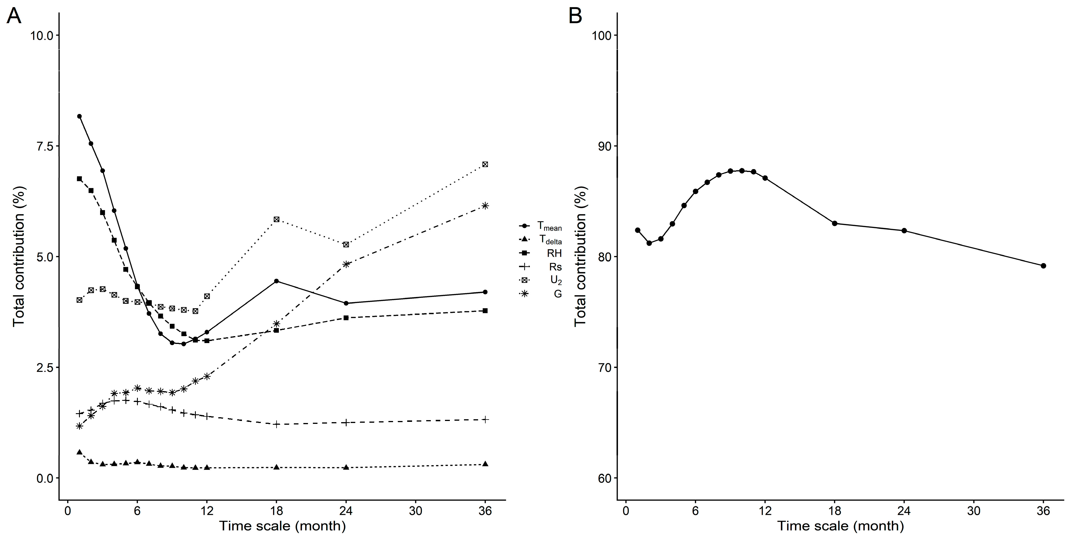
3.2.3. SPEI Sensitivity Analysis at Different Time Scales

Dynamic changes in the first-order and total sensitivity indices of the SPEI to T_mean, T_delta, RH, Rs, U₂, G, and P, respectively, as the time scale increases, are shown in Figure 6 and Figure 7. At the 1 month time scale, the first-order sensitivity values were from high to low as follows: P (80.6%) > T_mean (6.6%) > RH (5.3%) > U₂ (2.8%) > Rs (1.0%) > G (0.5%) > T_delta (0.1%). As the time scale increased, the sensitivity of T_mean experienced a rapid decline, and was followed by a slight increase. In particular, at the 1 to 12 month scale, the sensitivity to T_mean decreased rapidly from 6.6% to 3.0%, while at the 12 to 36 month scale, the T_mean increased slowly from 3.0% to 3.8% and subsequently stabilized. The sensitivity of T_delta was generally observed to be stable over the time scales, and within the range of 0–0.1%. The sensitivity of RH exhibited a similar trend to that of T_mean, with a decrease of 5.3% to 2.8% corresponding to the time scale increase from 1 to 12 month scale, and followed by a slight increase with further time scale increases up to 36 months. The sensitivity of Rs exhibited an initial increase with time scale (1 to 4 months), followed by a decrease (5 to 12 month scale), and finally stabilized (after 13 month scale). However, observed changes were relatively slight, ranging from 0.5% to 1.5% (Figure 6A). Both the first-order average sensitivities to U₂ and G exhibited a steady trend in variation with the time scale increases. At the time scale of 1 month, the sensitivity indices were 2.8% and 0.5%, and increased to 6.6% and 5.7%, respectively, at time scale of 36 months. The sensitivity index to P fluctuated between 78.4% and the maximum value of 87.2% (11 to 12 months) over all time scales, initially rising then declining. These values are much higher than those of other meteorological variables. The results suggest that the time scale has a significant impact on the sensitivity of the SPEI to meteorological variables in Jilin Province.

In summary, at the short time scale of 1 to 6 months, the order of the SPEI sensitivity was observed as follows: P > T_mean > RH > U₂ > Rs > G > T_delta. At the time scale of 7 to 18 months, the sequence was observed as: P > U₂ > RH ≈ T_mean > G > Rs > T_delta. For more than 24 months, the sequence was as follows: P > U₂ > G > T_mean > RH > Rs > T_delta.

4. Discussion

Numerous in-depth studies have recently been conducted in order to symmetrically evaluate SPEI characteristics over varying temporal and spatial scales [58,59]. However, investigations regarding the sensitivity of the SPEI are still relatively unclear. Previous findings regarding the sensitivity of the SPEI have been reported by Yao et al. [34] and Serrano et al. [35], but the variables are all limited to P and ET_o. This may be caused by the calculation of the SPEI giving a high frequency of 0 values [18] when the water is relatively balanced, which makes the nondimensional relative sensitivity coefficients (∂SPEI/∂x·x/SPEI) incalculable due to the “1/0 problem” when using the conventional-partial-derivative-based sensitivity analysis (a local sensitivity analysis method) [60,61]. In this study, a global sensitivity analysis, EFAST model, was therefore applied. The sensitivity of SPEI to meteorological variables at different temporal and spatial scales, as well as at different time scales, was discussed.

P is undoubtedly the most influential variable to the SPEI over time and space (Figure 3, Figure 4, and Figure 5). Our results suggested that P explains 59.9%–97.9% of the SPEI total variability in time from January to December, and 61.2%–94.9% in space with a gradient downward trend from the southeast to the northwest. In particular, during the main crop growing season (from May to September), P was the only sensitive variable identified (the relative sensitivity coefficient ranges from 87.1% to 97.9%), with all the other meteorological variables contributing a negligible amount of sensitivity coefficient (<5%) (Figure 3). In Tibet, China, Li et al. [62], using a multiple regression model, also reported that precipitation has the most significant influence on the variation of the SPEI. In addition, Zhang et al. [33], using the self-calibrating Palmer Drought Severity Index, confirmed our findings, and concluded that the sensitivity of precipitation was higher than that of ET_o. Our finding, the high contribution rate of P, would also be a potential evidence and explanation as to why the P-based indices like the SPI show a high level of consistency with the SPEI, and a considerable adaptability in most times and places, such as the findings of Yao et al. [34], Wang et al. [57], Chen et al. [8], and Przybylak et al. [30].

P is undoubtedly the most influential variable to the SPEI, while T_mean, RH, or U₂ observably affect the SPEI and cannot be neglected (Figure 3, Figure 4, and Figure 5). Sensitivity analysis models only involved P or P and ET_o may fail to consider the impact of T_mean, T_delta, RH, Rs, U₂, and G on drought in the context of global warming [12,35]. Our results using the EFAST model suggest that the SPEI was the most affected by P (80.6%), followed by T_mean (6.6%), RH (5.3%), U₂ (2.8%), Rs (1.0%), and T_delta (0.1%) for the Jilin Province as a whole. During the main crop growing season (from May to September), P was the only sensitive variable identified, but T_mean, RH, or U₂ observably affect the SPEI and cannot be neglected (the sensitivity coefficients ≥ 5%) during the nongrowing season (Figure 3). This result suggests that the SPEI may have an advantage over P-based indices such as the SPI and CZI, especially in the context of global warming, because other meteorological variables are not stationary, which made the assumptions of the SPI invalid [8]. The sensitivity of the SPEI to climatic variables differs not only in months, but also in spatial distribution [57]. Our findings further suggest that, in Jilin Province, the SPEI was mainly affected by P in the eastern region, while it was also influenced by T_mean, RH, and U₂ as well in the western region (Figure 4 and Figure 5). This may be due to relatively lower precipitation in the western plains where the ET₀ makes more contribution to water balance (P-ET_o), and thus explains a higher amount of the SPEI total variability. Regarding the order of sensitivities, Wang et al. [32] analyzed the impact of drought evolution on climate variables using the standardized regression coefficient and concluded that the most sensitive variable in south China, north China and the Qinghai-Tibet plateau was P, followed by U₂, T_mean, RH, and Rs. Moreover, in northwest China, the most sensitive variable was identified as U₂, followed by P, T_mean, RH, and Rs. These results are similar to those of our study, yet the order of sensitivities differs. This may be attributed to differences in the study areas and sensitivity models.

Numerous studies have demonstrated that the SPEI is both multi-scale and comprehensive. In particular, in the context of global warming, considering T_mean, T_delta, RH, Rs, U₂, G, and P, the SPEI is able to effectively identify different drought types [7,9,10,11]. However, the effects of T_mean, T_delta, RH, Rs, U₂, G, and P on the SPEI still remain unclear, especially at different time scales. Thus, we further investigated the sensitivity of SPEI with respect to meteorological variables at different time scales in Jilin Province. The specific time scales investigated were 1 to 36 months. The model was reconstructed in conjunction with the SPEI, and EFAST was applied for global sensitivity analysis on the SPEI. The EFAST model show that the sensitivity of the SPEI differs in time scales. At the time scale of 1 to 6 months, SPEI are the most sensitive to P, followed by T_mean, RH, U₂, Rs, G, and T_delta. At the time scale of 7 to 18 months, P is the most sensitive climatic variable to the SPEI, followed by U₂, RH, T_mean, G, Rs, T_delta. The order changes to P > U₂ > G > T_mean > RH > Rs > T_delta when the time scale increases up to more than 24 months. The significant response of SPEI to time scales is potentially caused by the multi-scalar phenomenon of the SPEI or drought. The SPEI at the 1 to 6 month time scale is most appropriate to monitor drought impacts with regard to meteorological and agroecological systems, while the SPEI at the 7 to 18 month time scale is appropriate for the drought identification for hydrological systems [8,9,63]. Some other authors also report that 1, 3, and 24 month time scales are used as a good proxy for meteorological, agricultural, and hydrological [30].

With more and more notable effects of global warming, the climate change impact on the SPEI is very complex. Our work focuses on a preliminary analysis of a possible tendency of climatic variables and the sensitivity of the SPEI in response to them, as well as the multi-scalar characteristics using the FAO-56 PM methods. The impact of the topographic feature on the SPEI and variations in SPEI resulting from different ET_o calculation methods, not considered in this study, should be investigated in future work.

5. Conclusions

Jilin Province experienced a significant rise in T_mean, and a sharp decrease in T_delta, Rs, and U₂ in the past 60 years. P is undoubtedly the most influential one to the SPEI among the seven selected meteorological variables, which explained 59.9%–97.9% of the total variability, especially during the main crop growing season (from May to September), while T_mean, RH, or U₂ observably affect the SPEI and cannot be neglected during the nongrowing season. In terms of spatial distribution, the SPEI was mainly affected by P in the eastern region, while it was also influenced by T_mean, RH, and U₂ as well in the western region. The sensitivity of the SPEI differs in time scales: P > T_mean > RH > U₂ > Rs > G > T_delta (1 to 6 month), P > U₂ > RH ≈T_mean > G > Rs > T_delta (7 to 18 month), and P > U₂ > G > T_mean > RH > Rs > T_delta (more than 24 month time scale), respectively. The results have the potential to provide a reference for agricultural production and management in Jilin Province, China.

References

1. Stocker, T.F.; Qin, D.; Plattner, G.; Tignor, M.; Allen, S.K.; Boschung, J.; Nauels, A.; Xia, Y.; Bex, V.; Midgley, P.M.; et al. Climate Change 2013: The Physical Science Basis; Cambridge University Press: Cambridge, UK, 2013. [Google Scholar]
2. Rojas, O.; Piersante, A.; Cumani, M.; Li, Y. Understanding the Drought Impact of El Niño/La Niña in the Grain Production Areas in Eastern Europe and Central Asia; FAO: Rome, Italy, 2019. [Google Scholar]
3. Wang, Y.; Zhao, W.; Zhang, Q.; Yao, Y. Characteristics of drought vulnerability for maize in the eastern part of Northwest China. Sci. Rep. 2019, 9, 964–969. [Google Scholar] [CrossRef] [PubMed] [Green Version]
4. Zhang, J.; Chen, H.; Zhang, Q. Extreme drought in the recent two decades in northern China resulting from Eurasian warming. Clim. Dyn. 2019, 52, 2885–2902. [Google Scholar] [CrossRef] [Green Version]
5. Abiodun, B.J.; Makhanya, N.; Petja, B.; Abatan, A.A.; Oguntunde, P.G. Future projection of droughts over major river basins in Southern Africa at specific global warming levels. Theor. Appl. Climatol. 2019, 137, 1785–1799. [Google Scholar] [CrossRef]
6. Ahmadalipour, A.; Moradkhani, H.; Castelletti, A.; Magliocca, N. Future drought risk in Africa: Integrating vulnerability, climate change, and population growth. Sci. Total Environ. 2019, 662, 672–686. [Google Scholar] [CrossRef]
7. Vicente-Serrano, S.M.; Beguería, S.; López-Moreno, J.I. A Multiscalar Drought Index Sensitive to Global Warming: The Standardized Precipitation Evapotranspiration Index. J. Clim. 2010, 23, 1696–1718. [Google Scholar] [CrossRef] [Green Version]
8. Chen, T.; Xia, G.; Liu, T.; Chen, W.; Chi, D. Assessment of Drought Impact on Main Cereal Crops Using a Standardized Precipitation Evapotranspiration Index in Liaoning Province, China. Sustainability 2016, 8, 1069. [Google Scholar] [CrossRef] [Green Version]
9. Gao, X.; Zhao, Q.; Zhao, X.; Wu, P.; Pan, W.; Gao, X.; Sun, M. Temporal and spatial evolution of the standardized precipitation evapotranspiration index (SPEI) in the Loess Plateau under climate change from 2001 to 2050. Sci. Total Environ. 2017, 595, 191–200. [Google Scholar] [CrossRef]
10. Miah, M.G.; Abdullah, H.M.; Jeong, C. Exploring standardized precipitation evapotranspiration index for drought assessment in Bangladesh. Environ. Monit. Assess. 2017, 189, 547. [Google Scholar] [CrossRef]
11. Moorhead, J.E.; Marek, G.W.; Gowda, P.H.; Marek, T.H.; Porter, D.O.; Singh, V.P.; Brauer, D.K. Exceedance Probability of the Standardized Precipitation-Evapotranspiration Index in the Texas High Plains. Agric. Sci. 2017, 8, 783. [Google Scholar] [CrossRef] [Green Version]
12. Stagge, J.H.; Tallaksen, L.M.; Xu, C.Y.; Van Lanen, H.A. Standardized precipitation-evapotranspiration index (SPEI): Sensitivity to potential evapotranspiration model and parameters. Hydrol. Chang. World 2014, 363, 367–373. [Google Scholar]
13. Wang, Q.; Shi, P.; Lei, T.; Geng, G.; Liu, J.; Mo, X.; Li, X.; Zhou, H.; Wu, J. The alleviating trend of drought in the Huang-Huai-Hai Plain of China based on the daily SPEI. Int. J. Climatol. 2015, 35, 3760–3769. [Google Scholar] [CrossRef]
14. Wang, W.; Zhu, Y.; Xu, R.; Liu, J. Drought severity change in China during 19612-012 indicated by SPI and SPEI. Nat. Hazards 2015, 75, 2437–2451. [Google Scholar] [CrossRef]
15. Tong, S.; Lai, Q.; Zhang, J.; Bao, Y.; Lusi, A.; Ma, Q.; Li, X.; Zhang, F. Spatiotemporal drought variability on the Mongolian Plateau from 1980--2014 based on the SPEI-PM, intensity analysis and Hurst exponent. Sci. Total Environ. 2018, 615, 1557–1565. [Google Scholar] [CrossRef] [PubMed]
16. Drumond, A.; Stojanovic, M.; Nieto, R.; Vicente-Serrano, S.M.; Gimeno, L. Linking anomalous moisture transport and drought episodes in the IPCC reference regions. Bull. Am. Meteorol. Soc. 2019, 100, 1481–1498. [Google Scholar] [CrossRef]
17. Zarei, A.R.; Moghimi, M.M. Modified version for SPEI to evaluate and modeling the agricultural drought severity. Int. J. Biometeorol. 2019, 63, 911–925. [Google Scholar] [CrossRef] [PubMed]
18. Beguería, S.; Vicente-Serrano, S.M.; Reig, F.; Latorre, B. Standardized precipitation evapotranspiration index (SPEI) revisited: Parameter fitting, evapotranspiration models, tools, datasets and drought monitoring. Int. J. Climatol. 2014, 34, 3001–3023. [Google Scholar] [CrossRef] [Green Version]
19. Peña-Gallardo, M.; Vicente-Serrano, S.M.; Quiring, S.; Svoboda, M.; Hannaford, J.; Tomas-Burguera, M.; Martín-Hernández, N.; Domínguez-Castro, F.; El Kenawy, A. Response of crop yield to different time-scales of drought in the United States: Spatio-temporal patterns and climatic and environmental drivers. Agric. Forest. Meteorol. 2019, 264, 40–55. [Google Scholar] [CrossRef] [Green Version]
20. Hargreaves, G.H.; Samani, Z.A. Reference crop evapotranspiration from temperature. Appl. Eng. Agric. 1985, 1, 96–99. [Google Scholar] [CrossRef]
21. Priestley, C.H.B.; Taylor, R.J. On the assessment of surface heat flux and evaporation using large-scale parameters. Mon. Weather Rev. 1972, 100, 81–92. [Google Scholar] [CrossRef]
22. Allen, R.G.; Pereira, L.S.; Raes, D.; Smith, M. Others Crop evapotranspiration-Guidelines for computing crop water requirements-FAO Irrigation and drainage paper 56. Fao Rome 1998, 300, D5109. [Google Scholar]
23. Chen, H.; Sun, J. Changes in Drought Characteristics over China Using the Standardized Precipitation Evapotranspiration Index. J. Clim. 2015, 28, 5430–5447. [Google Scholar] [CrossRef]
24. Li, X.; Sha, J.; Wang, Z. Comparison of drought indices in the analysis of spatial and temporal changes of climatic drought events in a basin. Environ. Sci. Pollut. Res. 2019, 26, 10695–10707. [Google Scholar] [CrossRef] [PubMed]
25. Trenberth, K.E.; Dai, A.; Van Der Schrier, G.; Jones, P.D.; Barichivich, J.; Briffa, K.R.; Sheffield, J. Global warming and changes in drought. Nat. Clim. Chang. 2014, 4, 17. [Google Scholar] [CrossRef]
26. Wang, Z.; Li, J.; Lai, C.; Zeng, Z.; Zhong, R.; Chen, X.; Zhou, X.; Wang, M. Does drought in China show a significant decreasing trend from 1961 to 2009? Sci. Total Environ. 2017, 579, 314–324. [Google Scholar] [CrossRef] [PubMed]
27. Reusser, D.E.; Buytaert, W.; Zehe, E. Temporal dynamics of model parameter sensitivity for computationally expensive models with the Fourier amplitude sensitivity test. Water Resour. Res. 2011, 47. [Google Scholar] [CrossRef] [Green Version]
28. Saltelli, A.; Ratto, M.; Tarantola, S.; Campolongo, F.; Commission, E. Sensitivity analysis practices: Strategies for model-based inference. Reliab. Eng. Syst. Saf. 2006, 91, 1109–1125. [Google Scholar] [CrossRef]
29. Enku, T.; Melesse, A.M. A simple temperature method for the estimation of evapotranspiration. Hydrol. Process. 2014, 28, 2945–2960. [Google Scholar] [CrossRef]
30. Przybylak, R.; Oliński, P.; Koprowski, M.; Filipiak, J.; Pospieszyńska, A.; Chorążyczewski, W.; Puchałka, R.; Dąbrowski, H.P. Droughts in the area of Poland in recent centuries. Clim. Past. Discuss. 2019, 15–16. [Google Scholar] [CrossRef]
31. Meijuan, Q.; Buchun, L.; Yuan, L.; Yueying, Z.; Xinyue, W.U.; Fuxiang, Y.; Dongni, W.; Chenying, M.U. Temporal-Spatial Variation Characteristics of Reference Crop Evapotranspiration and Its Influence Factors in Jilin Province. J. Arid Meteor. 2019, 37, 119–126. [Google Scholar]
32. Wang, Z.; Ye, A.; Wang, L.; Liu, K.; Cheng, L. Spatial and temporal characteristics of reference evapotranspiration and its climatic driving factors over China from 19792-015. Agr. Water Manag. 2019, 213, 1096–1108. [Google Scholar] [CrossRef]
33. Zhang, Y.; Li, G.; Ge, J.; Li, Y.; Yu, Z.; Niu, H. scPDSI is more sensitive to precipitation than to reference evapotranspiration in China during the time period 19512-015. Ecol. Indic. 2019, 96, 448–457. [Google Scholar] [CrossRef]
34. Yao, J.; Zhao, Y.; Chen, Y.; Yu, X.; Zhang, R. Multi-scale assessments of droughts: A case study in Xinjiang, China. Sci. Total Environ. 2018, 630, 444–452. [Google Scholar] [CrossRef]
35. Vicente-Serrano, S.M.; Van der Schrier, G.; Beguería, S.; Azorin-Molina, C.; Lopez-Moreno, J. Contribution of precipitation and reference evapotranspiration to drought indices under different climates. J. Hydrol. 2015, 526, 42–54. [Google Scholar] [CrossRef] [Green Version]
36. Manzano, A.; Clemente, M.A.; Morata, A.; Luna, M.Y.; Beguería, S.; Vicente-Serrano, S.M.; Martín, M.L. Analysis of the atmospheric circulation pattern effects over SPEI drought index in Spain. Atmos. Res. 2019, 230, 104630. [Google Scholar] [CrossRef]
37. Abbasi, A.; Khalili, K.; Behmanesh, J.; Shirzad, A. Drought monitoring and prediction using SPEI index and gene expression programming model in the west of Urmia Lake. Theor. Appl Climatol. 2019, 138, 553–567. [Google Scholar] [CrossRef]
38. Saltelli, A.; Tarantola, S.; Chan, K. A quantitative model-independent method for global sensitivity analysis of model output. Technometrics 1999, 41, 39–56. [Google Scholar] [CrossRef]
39. Wang, H.; Zhou, T.; Du, J.; Miao, Z. Application of Temperature-Vegetation Dryness Index in Monitoring Drought in the Jilin Province. Remote Sens. Technol. Appl. 2013, 28, 324–329. [Google Scholar]
40. Liu, D.; Guo, S.; Chen, X.; Shao, Q. Analysis of trends of annual and seasonal precipitation from 1956 to 2000 in Guangdong Province, China. Hydrol. Sci. J. 2012, 57, 358–369. [Google Scholar] [CrossRef]
41. Xu, Y.P.; Pan, S.; Fu, G.; Tian, Y.; Zhang, X. Future potential evapotranspiration changes and contribution analysis in Zhejiang Province, East China. J. Geophys. Res. Atmos. 2014, 119, 2174–2192. [Google Scholar] [CrossRef] [Green Version]
42. Hamed, K.H.; Rao, A.R. A modified Mann-Kendall trend test for autocorrelated data. J. Hydrol. 1998, 204, 182–196. [Google Scholar] [CrossRef]
43. Yue, S.; Pilon, P.; Phinney, B.; Cavadias, G. The influence of autocorrelation on the ability to detect trend in hydrological series. Hydrol. Process. 2002, 16, 1807–1829. [Google Scholar] [CrossRef]
44. Sen, P.K. Estimates of the regression coefficient based on Kendall’s tau. J. Am. Stat. Assoc. 1968, 63, 1379–1389. [Google Scholar] [CrossRef]
45. Marchetto, A. rkt: Mann-Kendall Test, Seasonal and Regional Kendall Tests. Available online: https://cran.r-project.org/web/packages/rkt/index.html (accessed on 12 February 2020).
46. Polong, F.; Chen, H.; Sun, S.; Ongoma, V. Temporal and spatial evolution of the standard precipitation evapotranspiration index (SPEI) in the Tana River Basin, Kenya. Theor. Appl. Climatol. 2019, 138, 777–792. [Google Scholar] [CrossRef]
47. Cukier, R.I.; Fortuin, C.M.; Shuler, K.E.; Petschek, A.G.; Schaibly, J.H. Study of the sensitivity of coupled reaction systems to uncertainties in rate coefficients. I Theory. J. Chem. Phys. 1973, 59, 3873–3878. [Google Scholar] [CrossRef]
48. Cukier, R.I.; Schaibly, J.H.; Shuler, K.E. Study of the sensitivity of coupled reaction systems to uncertainties in rate coefficients. III. Analysis of the approximations. J. Chem. Phys. 1975, 63, 1140–1149. [Google Scholar] [CrossRef]
49. Cukier, R.I.; Levine, H.B.; Shuler, K.E. Nonlinear sensitivity analysis of multiparameter model systems. J. Comput. Phys. 1978, 26, 1–42. [Google Scholar] [CrossRef]
50. Mesgouez, A.; Buis, S.; Lefeuve-Mesgouez, G.; Micolau, G. Use of global sensitivity analysis to assess the soil poroelastic parameter influence. Wave Motion 2017, 72, 377–394. [Google Scholar] [CrossRef] [Green Version]
51. Zhang, X.; Trame, M.N.; Lesko, L.J.; Schmidt, S. Sobol sensitivity analysis: A tool to guide the development and evaluation of systems pharmacology models. Cpt Pharmacomet. Syst. Pharmacol. 2015, 4, 69–79. [Google Scholar] [CrossRef]
52. Sobol, I.M. Global sensitivity indices for nonlinear mathematical models and their Monte Carlo estimates. Math. Comput. Simulat. 2001, 55, 271–280. [Google Scholar] [CrossRef]
53. Morris, M.D. Factorial sampling plans for preliminary computational experiments. Technometrics 1991, 33, 161–174. [Google Scholar] [CrossRef]
54. Lu, Y.; Mohanty, S. Sensitivity analysis of a complex, proposed geologic waste disposal system using the Fourier amplitude sensitivity test method. Reliab. Eng. Syst. Saf. 2001, 72, 275–291. [Google Scholar] [CrossRef]
55. Xu, C.; Gertner, G. Understanding and comparisons of different sampling approaches for the Fourier Amplitudes Sensitivity Test (FAST). Comput. Stat. Data Anal. 2011, 55, 184–198. [Google Scholar] [CrossRef] [Green Version]
56. Iooss, B.; Janon, A.; Pujol, G.; Broto, W.C.F.B.; Boumhaout, K.; Veiga, S.D.; Delage, T.; Fruth, J.; Gilquin, L.; Guillaume, J.; et al. Sensitivity: Global Sensitivity Analysis of Model Outputs. Available online: https://CRAN.R-project.org/package=sensitivity (accessed on 23 January 2020).
57. Wang, H.; Chen, Y.; Pan, Y.; Chen, Z.; Ren, Z. Assessment of candidate distributions for SPI/SPEI and sensitivity of drought to climatic variables in China. Int. J. Climatol. 2019, 39, 4392–4412. [Google Scholar] [CrossRef]
58. Jiang, R.; Xie, J.; He, H.; Luo, J.; Zhu, J. Use of four drought indices for evaluating drought characteristics under climate change in Shaanxi, China: 1951–2012. Nat. Hazards 2015, 75, 2885–2903. [Google Scholar] [CrossRef]
59. Zhao, H.; Gao, G.; An, W.; Zou, X.; Li, H.; Hou, M. Timescale differences between SC-PDSI and SPEI for drought monitoring in China. Phys. Chem. Earth Parts A/B/C 2017, 102, 48–58. [Google Scholar] [CrossRef]
60. McCuen, R.H. A sensitivity and error analysis of procedures used for estimating evaporation. Jawra J. Am. Water Resour. Assoc. 1974, 10, 486–497. [Google Scholar] [CrossRef]
61. Beven, K. A sensitivity analysis of the Penman-Monteith actual evapotranspiration estimates. J. Hydrol. 1979, 44, 169–190. [Google Scholar] [CrossRef]
62. Li, S.; Yao, Z.; Liu, Z.; Wang, R.; Liu, M.; Adam, J.C. The spatio-temporal characteristics of drought across Tibet, China: Derived from meteorological and agricultural drought indexes. Theor. Appl. Climatol. 2019, 11–16. [Google Scholar] [CrossRef]
63. Potop, V.; Ny, M.M.; Soukup, J. Drought evolution at various time scales in the lowland regions and their impact on vegetable crops in the Czech Republic. Agric. Forest. Meteorol. 2012, 156, 1211–1233. [Google Scholar] [CrossRef]
Figure 1. Spatial distribution of 28 meteorological stations in Jilin Province, China.
Sustainability 12 01713 g001
Figure 2. Spatial distribution of the trend of the main meteorological variables in Jilin Province, China, over the past 60 years, including Tmean (°C year−1) (A), Tdelta (°C year−1) (B), RH (%) (C), Rs (MJ m−2 d−1 a−1) (D), U2 (m s−1 a−1) (E), G (G, MJ m−2 d−1 a−1) (F), annual P (mm a−1) (G) and ETo (mm a−1) (H). The Theil–Sen approach was used to estimate the magnitude of time-series trends, while the Mann–Kendall nonparametric test was used to quantify the significance.
Sustainability 12 01713 g002
Figure 3. The first-order and the total sensitivity indices of SPEI to Tmean, Tdelta, RH, Rs, U2, G, and P in January (A), February (B), March (C), April (D), May (E), June (F), July (G), August (H), September (I), October (J), November (K), December (L), respectively, at 1 month time scale over the past 60 years for the Jilin Province as a whole.
Sustainability 12 01713 g003
Figure 4. Spatial distribution of the first-order sensitivity indices of the SPEI to Tmean (A), Tdelta (B), RH (C), Rs (D), U2 (E), G (F), and P (G), respectively, at 1 month time scale over the past 60 years in Jilin Province, China.
Sustainability 12 01713 g004
Figure 5. Spatial distribution of the total sensitivity indices of the SPEI to Tmean (A), Tdelta (B), RH (C), Rs (D), U2 (E), G (F), and P (G), respectively, at 1 month time scale over the past 60 years in Jilin Province, China.
Sustainability 12 01713 g005
Figure 6. The first-order sensitivity of the SPEI to Tmean, Tdelta, RH, Rs, U2, G (A), and P (B) to SPEI, respectively, at different time scales in Jilin Province, China.
Sustainability 12 01713 g006
Figure 7. The total sensitivity of the SPEI to Tmean, Tdelta, RH, Rs, U2, G (A), and P (B) to SPEI, respectively, at different time scales in Jilin Province, China.
Sustainability 12 01713 g007