All articles published by MDPI are made immediately available worldwide under an open access license. No special
permission is required to reuse all or part of the article published by MDPI, including figures and tables. For
articles published under an open access Creative Common CC BY license, any part of the article may be reused without
permission provided that the original article is clearly cited. For more information, please refer to
https://www.mdpi.com/openaccess.
Feature papers represent the most advanced research with significant potential for high impact in the field. A Feature
Paper should be a substantial original Article that involves several techniques or approaches, provides an outlook for
future research directions and describes possible research applications.
Feature papers are submitted upon individual invitation or recommendation by the scientific editors and must receive
positive feedback from the reviewers.
Editor’s Choice articles are based on recommendations by the scientific editors of MDPI journals from around the world.
Editors select a small number of articles recently published in the journal that they believe will be particularly
interesting to readers, or important in the respective research area. The aim is to provide a snapshot of some of the
most exciting work published in the various research areas of the journal.
In this paper, we address the problem of the efficient and sustainable operation of data centers (DCs) from the perspective of their optimal integration with the local energy grid through active participation in demand response (DR) programs. For DCs’ successful participation in such programs and for minimizing the risks for their core business processes, their energy demand and potential flexibility must be accurately forecasted in advance. Therefore, in this paper, we propose an energy prediction model that uses a genetic heuristic to determine the optimal ensemble of a set of neural network prediction models to minimize the prediction error and the uncertainty concerning DR participation. The model considers short term time horizons (i.e., day-ahead and 4-h-ahead refinements) and different aspects such as the energy demand and potential energy flexibility (the latter being defined in relation with the baseline energy consumption). The obtained results, considering the hardware characteristics as well as the historical energy consumption data of a medium scale DC, show that the genetic-based heuristic improves the energy demand prediction accuracy while the intra-day prediction refinements further reduce the day-ahead prediction error. In relation to flexibility, the prediction of both above and below baseline energy flexibility curves provides good results for the mean absolute percentage error (MAPE), which is just above 6%, allowing for safe DC participation in DR programs.
The energy demand of data centers (DCs) is rapidly growing, and studies have shown that, in 2014, worldwide, they consumed 194 TWh of electricity (about 1% of the global electricity demand). These numbers are expected to increase to 3% by 2025 [1,2]. Cloud architectures and services have undergone massive development in the last decade; thus, DCs’ energy demands have greatly increased, putting lots of pressure not only on their economic sustainability and environment impact but at the same time on the safe operation of the local energy grids to which they are connected, culminating in instability in the electricity network and severe risk of supply shortage [3]. Thus, in the past decade, a lot of industry efforts have concentrated on developing technologies for increasing the energy efficiency of DCs’ operation with a view to decreasing their energy demand [4,5,6].
The advent of intermittent decentralized renewable energy sources (RES) is completely changing how grids are managed, increasing the need for demand response (DR) programs and energy storage to maintain grid balance and power quality [7]. The DR programs, where they are truly integrated within local energy systems, may represent a first significant option for transforming energy consumers into flexible, active energy users and integrating them in the emerging energy system. At the same time, this may bring significant benefits to the smart grids, since it allows a Distribution System Operator (DSO) to procure, in a cost-effective way, the necessary energy flexibility for integrating larger shares of intermittent RESs and stabilize the grid while not compromising the security of supply and network reliability. For example, in Europe, studies have revealed that the EU peak demand could be reduced by 60 GW (approximately 10% of the EU’s peak demand) through DR measures [8]. However, to achieve a significant impact on load, flexibility schemes will require the dispatching of set-points to a greater number of assets and during a broader timeframe for 24 hours of a day. This inherently requires the introduction of engagement strategies for new types of energy customers (such as DCs) and the overtaking of technological barriers such as the accurate forecasting of demand, generation, and flexibility. Few studies have approached the efficient integration of DCs with the local energy grids via direct participation in DR programs; most of them focused on increasing the utilization of on-site renewable energy to take advantage of low energy prices [9,10]. To participate in DR programs, the DCs must accurately forecast their demand and potential flexibility and also optimally manage their operation to follow a DR signal provided by the DSO directly or by a flexibility aggregator [11]. As a result, the DCs can contribute to the stability of the local grid and can obtain a new income source besides their main revenue streams.
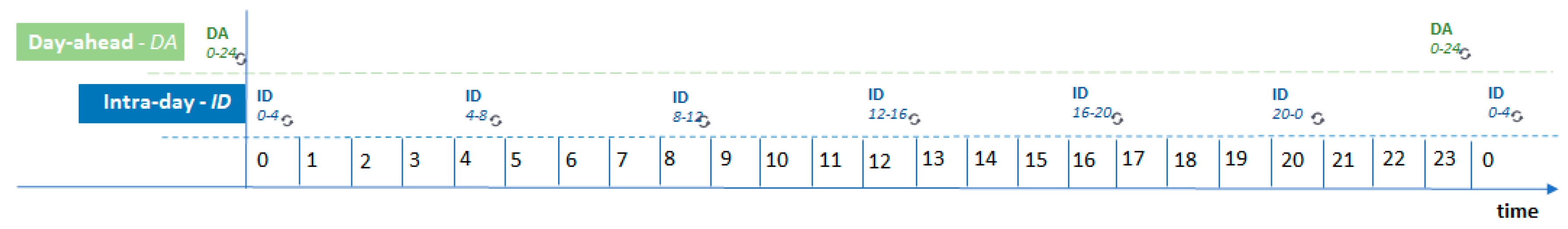
To show the technological barrier for DC participation in DR programs, we have considered contemporary DR scenarios, such as those described in reference [12]. The DC should act as a prosumer of electrical energy that has established flexibility purchase contracts with a Flexibility Aggregator in order to alleviate the associated risks with flexibility provisioning to its core business. The contract includes the operating conditions for the flexibility delivered by the DC in DR programs and the details of the financial settlement. Flexibility trading can be achieved daily, as shown in Figure 1. The DC must forecast its energy demand for the next day and send those values to the Flexibility Aggregator, which will collect this kind of information from its entire portfolio of prosumers in order to provide it to the DSO. The DSO will use the energy demand figures to detect potential congestion points, and if such congestion is forecasted for the next day, it will send a flexibility request to the Flexibility Aggregator. Upon aggregator request, DC must forecast its energy flexibility values for the next day in relation to a calculated baseline energy consumption. These values are then used by the Flexibility Aggregator to issue a flexibility order as a DR signal in terms of the DC energy demand profile that must be accurately followed in the next day to get rewarded, otherwise being at risk of penalty charges. During the operational day, these steps can be repeated considering a 4-h-ahead time frame.
As highlighted above, besides flexibility shifting and operation adaptation, the accurate forecasting of DCs energy demand and flexibility are key technical barriers for DCs’ enrolment and successful participation in DR programs. Moreover, poor energy consumption analytics and lack of forecasting tools are mentioned in literature as major barriers for DR programs adoption [13]. There are lots of factors that may influence DC energy demand forecasting outcomes such as the size of the training data set, the specific behavior of the system (quantity of noise, seasonality, trend, susceptibility of external factors, etc.), the level of data aggregation, the intrinsic parameters of the model used, the granularity at which the predictions are realized (minutes, hours, months, years) and the dimension of the prediction window (the number of steps in the future) [14,15,16]. In-depth analysis of prediction outcomes shows that some DC energy consumption prediction models can outperform others on some specific data sets and give poor results on others depending on data characteristics. Even on the same data set, with of relatively good prediction accuracy, big discrepancy may occur between the quality of the results for different time intervals. At the same time, to our knowledge, there is no relevant state of the art approach addressing the forecasting of DC energy flexibility in relation to the baseline load.
In this paper we address the limitations identified in the literature for energy demand and flexibility forecasting by defining a DC energy prediction model that uses a genetic heuristic to determine the optimal ensemble of a set of neural network-based prediction models to obtain a high energy forecasting accuracy. It addresses holistically a mix of time horizons needed for DC participation in DR programs (i.e., day-ahead and intra-day) as well as different aspects of energy such as energy demand and energy flexibility.
Thus, the contributions of this paper are the following:
Implementation of an ensemble-based DC energy prediction model that combines a set of individual neural network weak learners to forecast the DC energy demand for the next day and to refine it continuously considering four-hour intervals.
Definition of energy flexibility in relation to the baseline load and a prediction model to forecast the potential DC energy flexibility to be used in DR programs.
Implementation of a genetic heuristic to determine the optimal combination of the outcome of individual predictors to minimize the prediction error thus lowering the uncertainty concerning DR participation.
The rest of the paper is structured as follows: Section 2 presents state of the art approaches on energy prediction related to DR programs, Section 3 describes the ensemble-based prediction model for DC energy demand and energy flexibility, Section 4 shows prediction results on a medium-scale DC testbed, while Section 5 concludes the paper and presents future work.
2. Related Work
Few state-of-the-art approaches address the topic of DC energy forecasting for DR participation, most of them being focused on energy demand and none, to our knowledge, addresses the forecasting of energy flexibility. Dayarathna et al. [17] conducted a survey of techniques for DCs energy consumption modelling and energy demand forecasting. Besides identifying the IT equipment and facility infrastructure as the main consumers they classified existing machine learning-based approaches for DC energy consumption forecasting. They concluded that existing research work concentrated more on studying the energy efficiency of lower hardware levels of DCs, but less on higher aggregated levels which is desired for DR programs. Google’s researchers [18] have trained a generic three-layered neural network on DCs to predict the power usage effectiveness (PUE) ratio, showing that prediction methods could be an effective way to model DCs performance that could bring significant cost savings on the global energy market. They achieved a 40% reduction in the amount of energy used for cooling their DC. Several DC energy prediction models are proposed, most of them targeting the increase of energy efficiency of DC operation [19,20] in isolation, without considering smart energy grid integration. Similarly, multi-objective genetic algorithms can be used to dynamically forecast resource usage and energy consumption in DCs [19]. They can forecast the resource requirements for a future time slot according to the historical data in previous time slots which is fed as input for virtual machines placement algorithms having as general objective the decrease of DC energy consumption. In [20] the authors present a DC power prediction framework based on power profiling and deep learning models. For short-time forecasting, a recursive autoencoder is used onto fine-grained models while for long-term prediction massive fine-grained historical data are encoded into the coarse-grained model. According to [21] the intermittent nature of renewable energy sources is seen as a major drawback of using it on DCs site. The authors propose a scheduler that uses IT and electrical models of the DC energy consumption together with an energy availability prediction engine for the next 48 h. In [22] a multi-layered ANN is defined and used to forecast the DC energy consumption on monthly intervals based on the historical energy consumption data. The forecast engine is implemented using MLP. Considering stability over prediction accuracy, in [23] a forecasting model that uses dynamic adaptive entropy-based weighting for total energy demand forecasting is proposed. The model combines classic prediction techniques such as Holt-Winters Multiplicative algorithm and moving average, using a weighted based ensemble. Finally, in one of our previous works [24] we proposed and successfully used neural network prediction models to forecast the DC server room temperature which is then used as input into the thermodynamics processes simulations to decide on adapting DC thermal energy profile for providing on-demand heat to nearby neighborhoods.
There are a lot of approaches in the literature that address energy consumption forecasting of regular prosumers. The most important ones are the deep neural network energy forecasting models, which are often used for medium and short-term predictions due to their low time overhead while raising concerns for their accuracy and creating the need for extensive comparative evaluation on similar energy sets [25]. In [26], the authors propose a novel building energy load forecasting methodology based on deep neural networks, more specifically long short-term memory (LSTM), which achieves accurate energy predictions, both at the aggregate and individual site level. For improving the forecasting results they investigate a LSTM architecture that maps sequences of different lengths. LSTM energy prediction models are compared with other machine learning-based approaches showing good improvements in terms of forecasting accuracy [27]. In [28] the authors argue that existing methods are not able to model the uncertainty at the prosumer level due to the many fluctuations in influencing variables which negatively impact the forecasting process. Consequently, deep extreme learning models are proposed for improving the performance of energy consumption forecasting [29,30,31]. In [32], artificial neural networks (ANNs) are used for accurate short-term load prediction based on smart meters gathered data; in the same time, they investigate different approaches for load aggregation. The authors of [33] propose an ANN-based approach for predicting energy usage of buildings, additionally considering the users’ characteristics and their activities as relevant features. In [34,35], an ANN model is proposed for carrying out day-ahead power predictions that on a specific scenario performs better than several other tested methods such as support-vector machine (SVM) and multilayer perceptron (MLP). The results show that the approach is suitable for assessing DR load shifting options based on a time-of-use pricing scheme achieving district level cost savings of around 15%. In [36], three types of deep learning-based energy-related features are compared with conventional feature engineering methods using fully connected auto-encoders, convolutional autoencoders, and generative adversarial networks. The authors of [35] use deep learning models to predict electricity consumption for arbitrary time horizons, by dividing each predicted sample into a single forecasting sub-problem which is solved independently by identifying the best forecasting model.
In the context of DR programs hybrid ensemble-based approaches can obtain better results for complex models [37]. The authors of [38] propose a hybrid SVM model to forecast the hourly electricity demand of buildings while several articles report good energy forecasting results using hybrid models of convolutional neural network (CNN) and LSTM [39,40,41]. In [42], multiple CNN components are employed to extract rich features from the historical load sequence and an LSTM based recurrent neural component is used to model the variability and dynamics of historical energy data. In [43] a hybrid network is described, which can extract spatial-temporal information and irregular features of electric power consumption to effectively predict building energy consumption while [44] defines a hybrid model between LSTM and recurrent neural network (RNN) to forecast the short- and medium-term aggregated load in micro-grids providing good results in the case of medium to long-range forecasting. A hybrid forecasting model that combines wavelet transform, Particle Swarm Optimization (PSO) and SVM for estimating short-term (one-day-ahead) generation power of a real micro-grid is proposed in [45]. Similarly, a hybrid model for electricity load and price forecasting based on a combination of Stochastic Gradient Descent and SVM that shows improved prediction accuracy is the subject of [46]. Other approaches use deep belief network to forecast the hourly load of the power grid [47] and combine chicken swarm optimization algorithm with SVM to make predictions on short-term wind power and improve the stability of power system operation reporting a better convergence and accuracy compared with other bio-inspired models [48].
Our approach builds upon the existing state of the art by proposing an ensemble-based DC energy prediction model for determining the DC energy demand and flexibility for 24- and 4-hour intervals for their active participation in DR programs. To our knowledge, even though such ensemble models give good results for different prosumers energy prediction, they have never been used to the specific case of DCs. Moreover, existing approaches are focused on forecasting the energy demand of prosumers and do not address other relevant aspects in DR such as the forecasting of energy flexibility. To determine the optimal combination of individual neural network model’s energy prediction outcomes we have used a genetic heuristic aiming to minimize the overall prediction process error, thus decreasing the uncertainty in relation to the successful participation of DCs in DR programs.
3. DC Energy Prediction Model
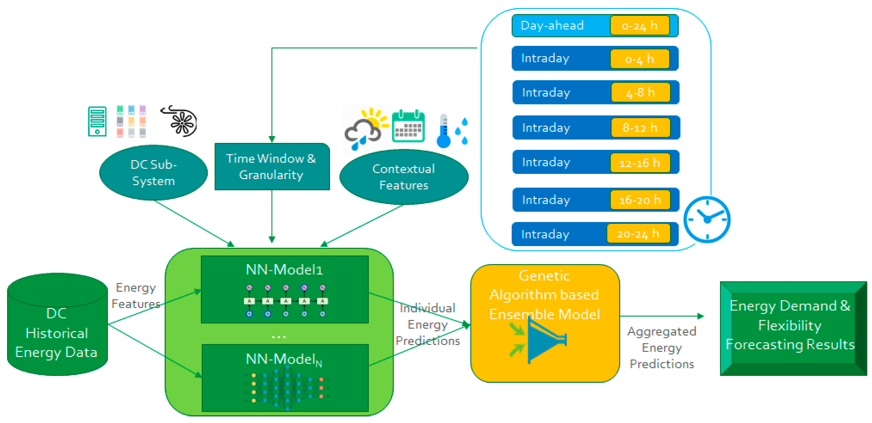
We propose an ensemble-based DC energy prediction model that aggregates the prediction outcomes of individual neural network based weak learners to forecast the DC energy demand and their potential energy flexibility. We have chosen neural networks due to their ability in modeling complex non-linear processes such as the energy exchange processes occurring inside a DC. At the same time the ensemble-based predictors seem to perform significantly better compared to individual algorithms for time series prediction tasks. The output of the weak learners is combined using a weighted average (see Figure 2) to improve the final prediction result. We have implemented genetic algorithm-based ensemble method to determine the optimal weights that will generate the best combined outcome for the specific DC energy prediction problem, considering both the characteristics of the input data and the interrelations among different DC sub-systems.
Each individual predictor can be defined as a function with parameter that computes the predictions based on the input energy data of a DC energy sub-system (), for a specific future time frame window and granularities :
Analyzing the DC energy demand and flexibility patterns of various DCs we have selected the IT servers and cooling sub-systems which are the major contributors to the DC total energy demand, as relevant sub-systems for the energy forecasting process. There is a strong dependency between the energy demand and flexibility potential of the IT servers and cooling sub-systems which need to be captured in the prediction model (see Figure 3). If the IT server’s sub-system has a higher energy demand, it will generate more heat and more cooling will be needed to maintain the temperature setpoints, generating an increase of energy demand from the cooling sub-system. Similarly, if the IT servers’ energy demand decreases, the cooling energy demand will also decrease.
The ensemble predictor gathers the results of each individual predictor and combines them based on evolutionary computing optimized weighted average to predict the final outcome:
where represents the weights vector that is applied to each individual predictor to obtain the best prediction performance and is the number of individual predictors.
The goal is to determine the parameters and such that the error between the energy predicted value and the actual monitored one is minimized for the entire forecasting time window:
3.1. Demand Forecasting
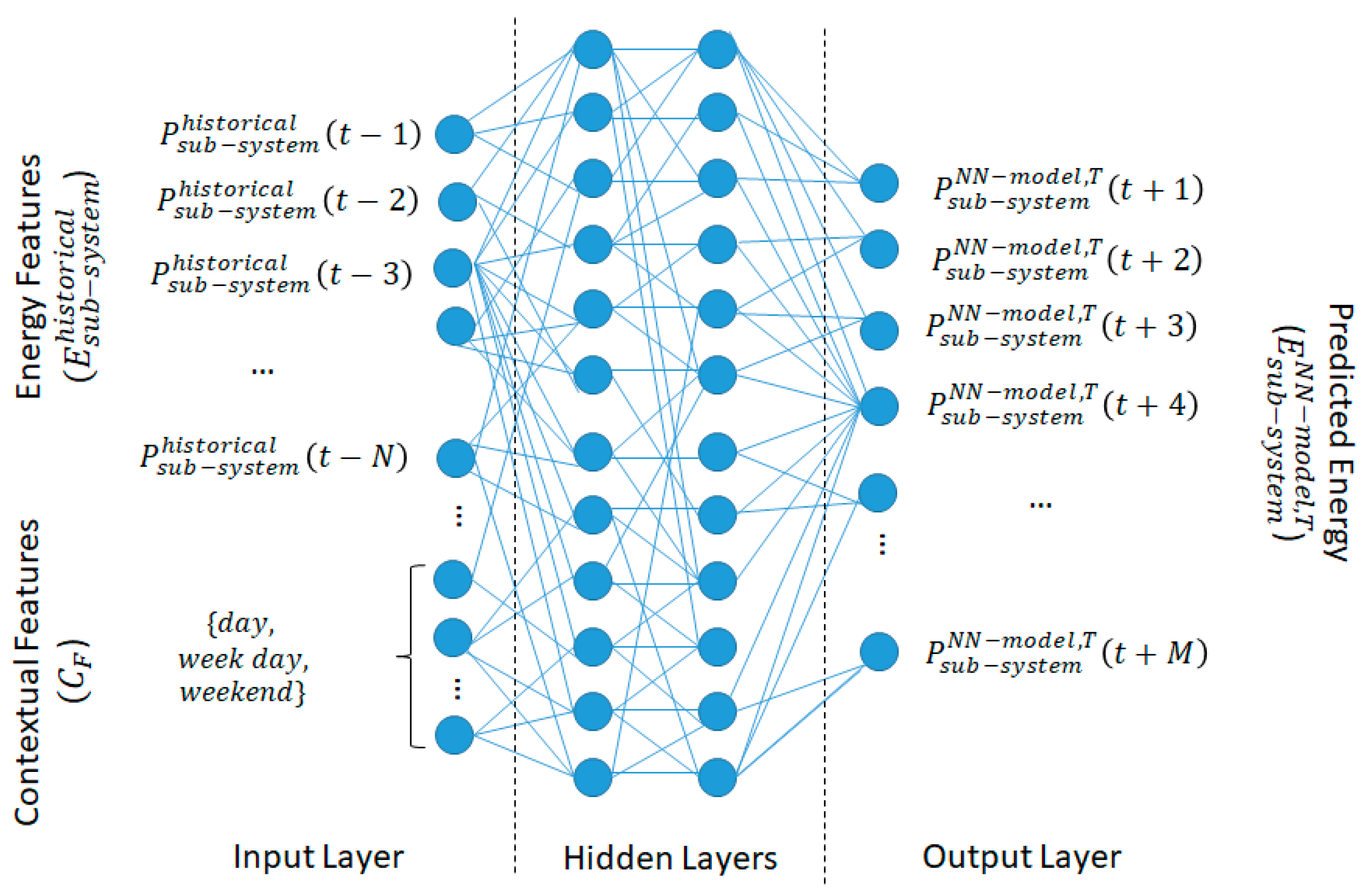
Each individual neural network is generically modeled as a set of neurons distributed over several hidden layers trying to map the energy inputs to outputs through a non-linear function (see Figure 4). Each model is then configured according to the forecasting time window, being fed with number of historical energy data inputs and additionally with the contextual features , and will predict number of future energy values.
We denote , the instant power value of a DC sub-system at timestamp . The energy of a DC sub-system on the time interval is denoted as and is defined as the integral of power over the time interval:
Because the prediction models use energy features sampled at equidistant timestamps, we define a discrete time model over which predictions are represented as a series of equidistant points on the time axis where the energy values are sampled:
The power values of each DC sub-system will be computed from monitored power values on equal and continuous time intervals spreading between equidistant timestamps:
The length of all intervals is constant, defined as or the time granularity of the sampling process. Considering the above, the energy on a time interval is computed using a basic interpolation technique as the average of the power values sampled by the monitoring infrastructure in the same interval:
Our model can consider several target variables, and can reduce the DC energy prediction problem (at different time windows) to a univariate multi-step forecasting problem as follows:
where is the prediction of a certain energy value at time from the forecasting time window with a granularity , represents the contextual features considered in the forecasting process, is the historical energy value at time used as input in the forecasting process, is the number of historical energy values used as inputs and is the size of the forecasting time window .
Analyzing current DR programs operation, we have identified that two-time horizons are relevant (see Figure 5) for potential usage of forecasting results to enact the DC to participate as a prosumer:
Day-ahead: energy values are forecasted for the next 24 h with a granularity of one hour;
Intra-day: energy values are forecasted for the next 4 h with a granularity of half an hour;
In the day-ahead case, the prediction model must forecast the hourly energy values for the next day, (i.e., 24 steps ahead), while the energy features considered are defined as historical energy data values spreading from the present to 24 h in the past, with time intervals granularity of one hour:
In the intra-day case, the prediction model must forecast energy values over a four-hour time interval at a 30-min granularity (i.e., 8 steps ahead), while the energy features considered are defined as historical energy data values spreading from the present to 4 h in the past, at intervals of half an hour granularity:
The energy-based features are further enhanced by adding contextual information as input, as we expect different energy profile patterns at different time contexts. Using them together with the energy value derived features, more complex and, maybe, hidden consumption patterns can be found. The contextual features represent data that are not specific to energy but correlated to context, such as season, weekdays and calendar days:
Season—the DC may consume/produce different quantities of energy depending on the season. For example, the energy consumption in summer can be higher than the energy consumption in winter especially due to more intensive use of cooling processes. Same reasoning may apply if we consider the renewable energy generation (i.e., solar energy). The possible values for this feature are: Spring, Summer, Autumn and Winter.
Day of the week—a DC may consume different quantities of energy depending on the day of the week. For example, the energy consumption for Monday may be higher than the energy consumption in a weekend day such as Saturday if the DC is running banking tasks. Possible values for this feature are Sunday, Monday, Tuesday, Wednesday, Thursday, Friday, Saturday.
Weekend—a DC may consume different quantities of energy depending on whether it is weekend day or not.
3.2. Flexibility Forecasting
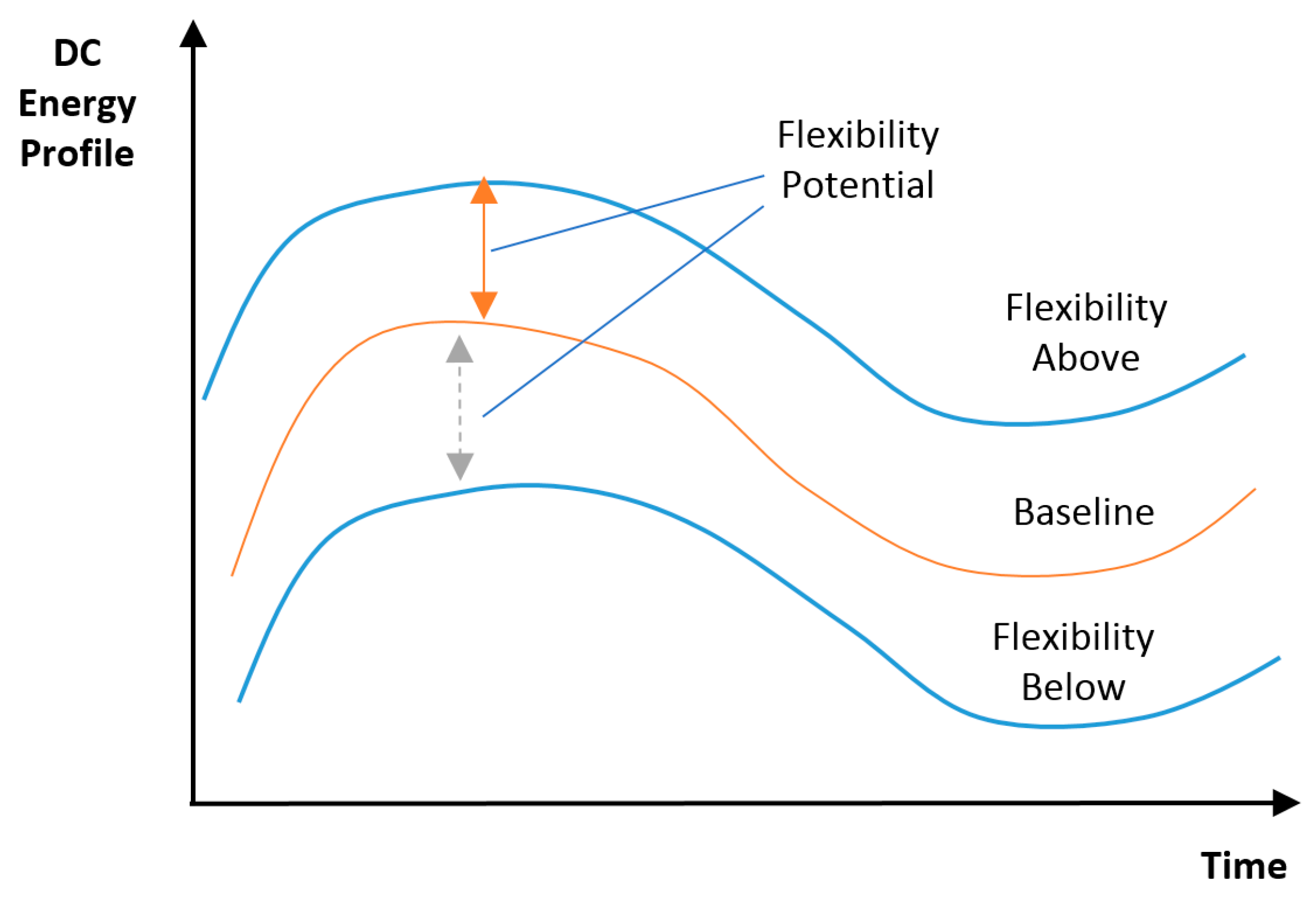
The energy flexibility of a DC measures the potential of adapting its energy demand in relation to a calculated baseline by shifting energy and, as a result, increasing or decreasing its energy demand profile. The baseline energy consumption is an estimate of the electricity that would have been consumed by each DC individual sub-system, or by the entire DC in the absence of any flexibility provisioning optimization. The baseline energy consumption profiling uses similar time scales as the energy demand forecasting process, but it is fundamentally different as it must satisfy both consumers and utility sides [49] and it is used only to measure the performance of the DC participation into a DR program. To determine the baseline at sub-system level we have used the X of Y method that calculates the baseline using the energy consumption data of Y previous days out of which the most significant X days are selected [50]. The average model-middle selects X days with the average load, excluding both the highest and the lowest loads, if they are isolated events. In this way the baseline is much more stable, and the error with respect to the load is reduced, but in this case, the actual energy demand may exceed the baseline at times:
The bigger the Y parameter is, the more samples will be needed, which this usually increases the effectiveness of estimation. But if Y is too big it could cause problems, such as being affected by the change in the characteristics of the workload run by the DC. Thus, in our model we have used .
Considering the calculated baseline, we aim to forecast the DC energy flexibility for the day-ahead and intra-day timeframes. To estimate the degree in which the DC can increase or decrease the load in a DR program using its internal latent flexibility and to measure the adaptation during the program in a time interval , we have used the adaptability power curve (APC) metric defined in the context of the EU Smart City Cluster [51]:
The APC metric computes the Manhattan distance between the actual and baseline energy profile vectors and normalizes it using the total power demand over the DR program time interval . The APC metric is defined for each DC sub-system and for the entire DC.
Considering this metric, we define for each DC sub-system over a timeframe at granularity , the flexibility above as the energy consumption values that are higher than the baseline and the flexibility below as the energy consumption values lower than the baseline:
The flexibility above and below profiles as well as the baseline for a DC sub-system over a period of 24 h is illustrated in Figure 6. The difference between the above profile and baseline as well as the difference between the baseline and below profile provide the energy features for the machine learning algorithms used to forecast the energy flexibility of each DC sub-system.
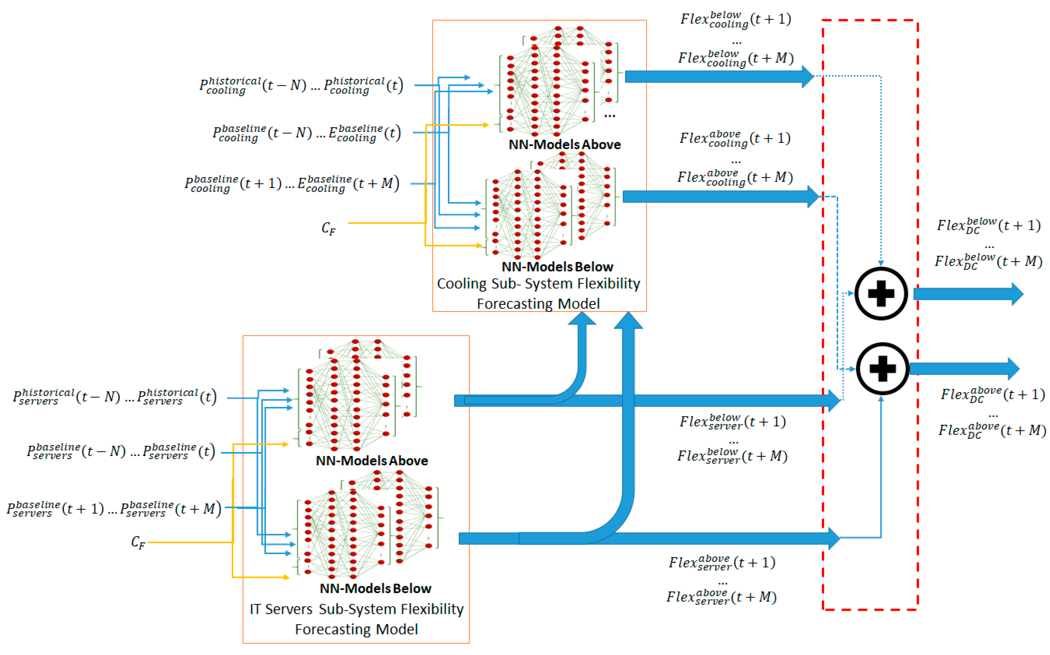
The flexibility forecasting aims to determine the demand flexibility of each DC sub-system over future timestamps at granularity based on a set of historical values of the considered features. The main sources of energy demand flexibility in a DC are the IT servers and cooling sub-systems. We have considered which other components that may deliver certain flexibility levels such as the auxiliary energy storage devices - are included in the flexibility profiles of the above-mentioned sub-systems. Following the energy relation between the DC sub-systems (see Figure 7) the cooling system flexibility forecasting model has the output generated by the server room flexibility forecasting model as input. Each individual sub-system flexibility model has the historical monitored energy consumption values, the baseline values over the previous time steps and the estimated baseline for the next time steps as inputs while their outputs are aggregated to compute the total DC energy demand flexibility.
Each sub-system flexibility model is implemented using two neural networks, used to predict either the flexibility below the baseline ( or the flexibility above the baseline (. We have considered that the individual neural networks models have similar characteristics, being composed of an input layer, two hidden layers with neurons each and an output layer with neurons.
3.3. Genetic Algorithm Based Ensemble
The DC energy prediction result over a specific forecasting time interval is calculated using a weighted average as:
where is the number of individual weak learners and is the weight of the energy prediction outcome generated by the considered in the ensemble process:
To determine the optimal values of weight matrix (i.e., the best combination of weights <> for each timestamp ) while taking into account the characteristics of the energy input data, prediction goal and energy interrelations between different subsystems of the DC, we will use a genetic algorithm. The sum off all weights for each timestamp in the interval should be equal to 1:
We have modeled each individual chromosome of the genetic algorithm as a vector:
representing a potential DC energy prediction weighted ensemble configuration. The entire population with individuals is defined as:
We define the fitness function aiming to minimize the MAPE of a potential weighted energy prediction ensemble and the actual monitored energy data:
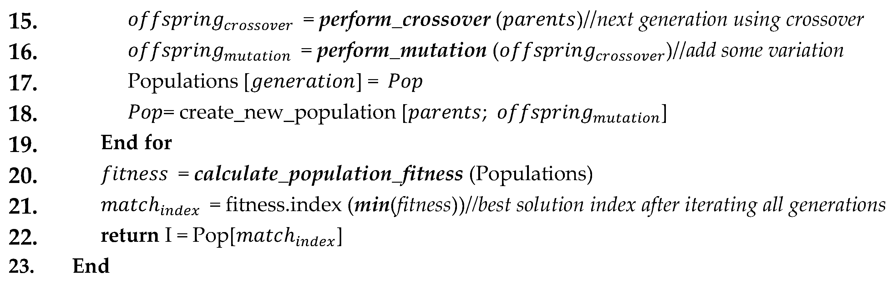
The pseudocode for the evolutionary optimized ensemble is presented in Figure 8. Each chromosome in the genetic algorithm has several genes corresponding to the length of forecasting time window (number of timestamps considered): 24 in the case of day-ahead, and 8 in the case of intra-day. Initially the individuals are randomly created by generating a random weight vector (line 11) for each gene corresponding to the timestamp .
Then, for each new generation the fitness function is computed for all individuals in the population (lines 12–13). The individuals with the best fitness value are selected as parents and mates for the next population generation (line 14). Using the crossover operation, the new individual offspring is calculated having its first half of genes taken from the first parent and the second half from the second parent ( being defined at the center):
Next, several genes are selected for mutation. A random value is added/subtracted from every individual prediction model weight at a certain position determined randomly (index of the gene) such that the mutation would maintain the constraint defined in relation (20):
New populations are created based on the parents and offspring, re-iterating through the process until the maximum number of generations defined is reached (lines 15–18). In the end, the algorithm will return the best individual from the population which will contain the encoding of the ensemble weight matrix for each timestamp of the forecasting time window .
4. Experimental Results
We have conducted a set of in-lab experiments to estimate the potential of our DC ensemble-based energy forecasting engine to generate accurate energy demand and energy flexibility predictions enacting the DCs to participate in DR programs. The prediction results are calculated in the day-ahead and intra-day forecasting time window and communicated on demand to the DSO for allowing it to accurately construct next day prognosis in the micro grid and potentially detect congestion points. For evaluation purposes we have considered the hardware characteristics as well as the historical energy consumption data of a medium scale DC (see Table 1) [52].
Figure 9 shows the historical energy demand values for the DC split into IT servers and cooling sub-systems. The data values range over a period of 3 months with a sampling rate of 10 min. The initial data have been split into 80% for training and 20% for testing purposes. Out of the training data, 20% has been kept for training the genetic algorithm and has not been presented to weak learners in order to avoid prediction model overfitting. The ensemble has been evaluated on the 20% of data kept for testing purposes.
We have considered two types of individual neural network models (i.e., differentiated by the neuron types) as mathematical functions used for regression, aiming to forecast energy values over a future time window: (i) MLP that uses rectified linear units (ReLU) [53] and (ii) LSTM [54]. The MLP has proven its suitability for regression problems because it can be seen as a logistic regressor that is fed through an intermediate layer called “hidden layer” activated by a non-linear function. LSTM has gained popularity due to its capability to learn long-term dependencies in time series data and to scale up to several layers of LSTMs.
The DC energy prediction models have been implemented in Python programming language using the TensorFlow learning library, making use of the integrated Keras API. Experiments have been carried out on a system equipped with an Intel Core i5 7600 K CPU 3.80 GHz, 24 GB RAM internal memory and an NVIDIA GeForce GTX 1050 GPU.
4.1. DC Energy Demand Prediction Results
We have evaluated the performance of the implemented energy prediction model for forecasting the DC energy demand considering both day-ahead and intra-day forecasting time horizons. Each neural network model (i.e., NN-model) has been configured according to the energy features of the DC sub-systems and the timeframe for which the prediction must be computed. The number of inputs, outputs, hidden layer and neuron types is presented in Table 2.
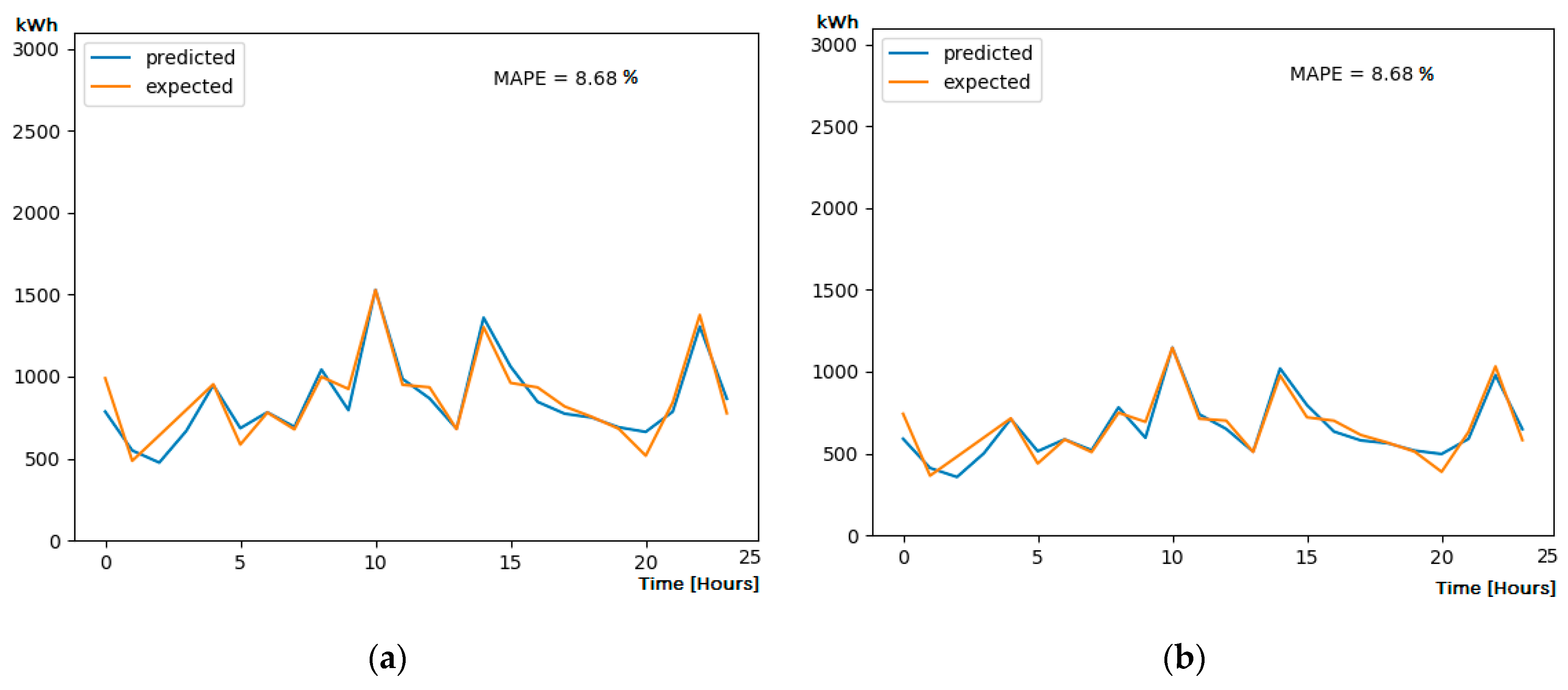
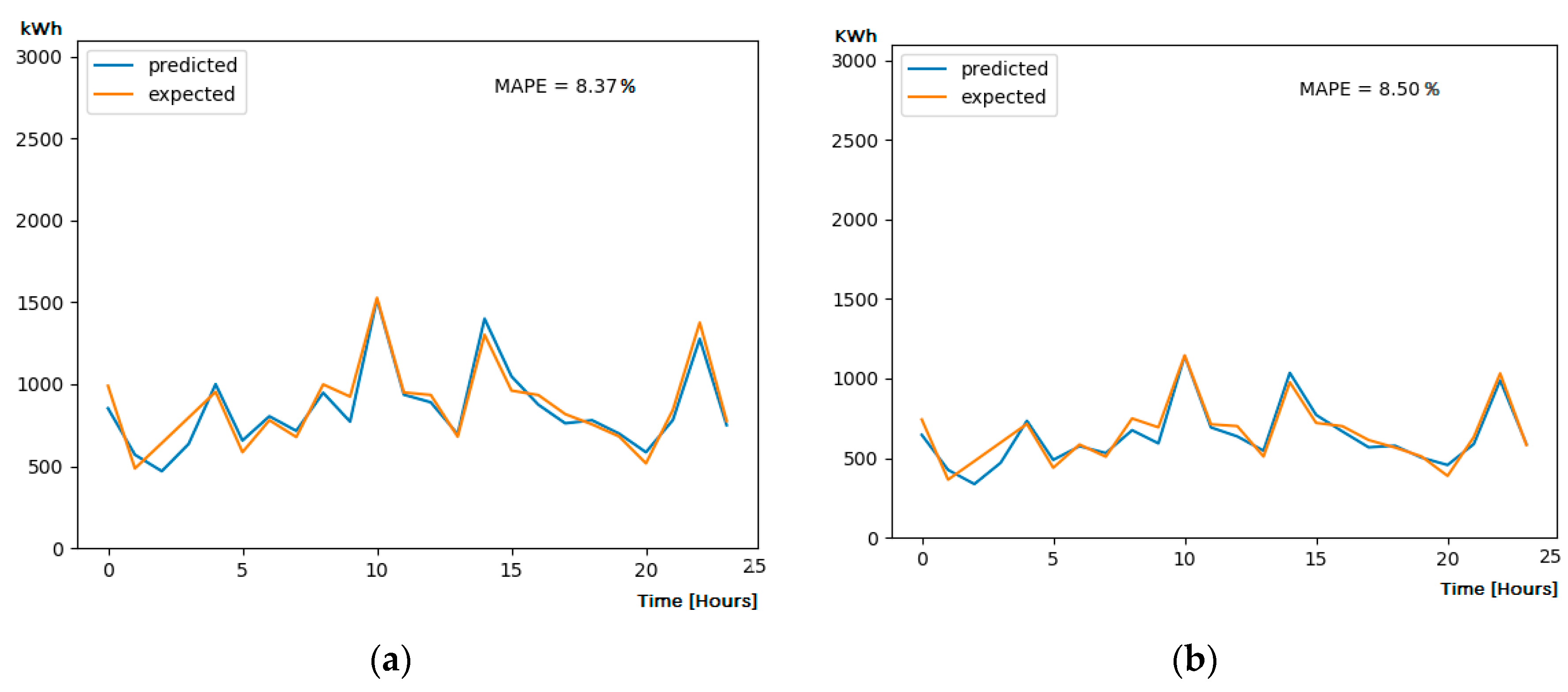
The first set of experiments aim to evaluate the performance of the ensemble predictor considering the day-ahead prediction framework and the results obtained over the test days by the MLP and LSTM neural networks.
Figure 10 and Figure 11 present details on the best forecasting results (i.e., best day from the testing set) obtained in terms of predicted energy profile compared with the actual one for different configurations of the forecasting models. The MAPE values for both type of weak learners considered are above 8% (i.e., 8.68% for MLP and 8.50% for LSTM).
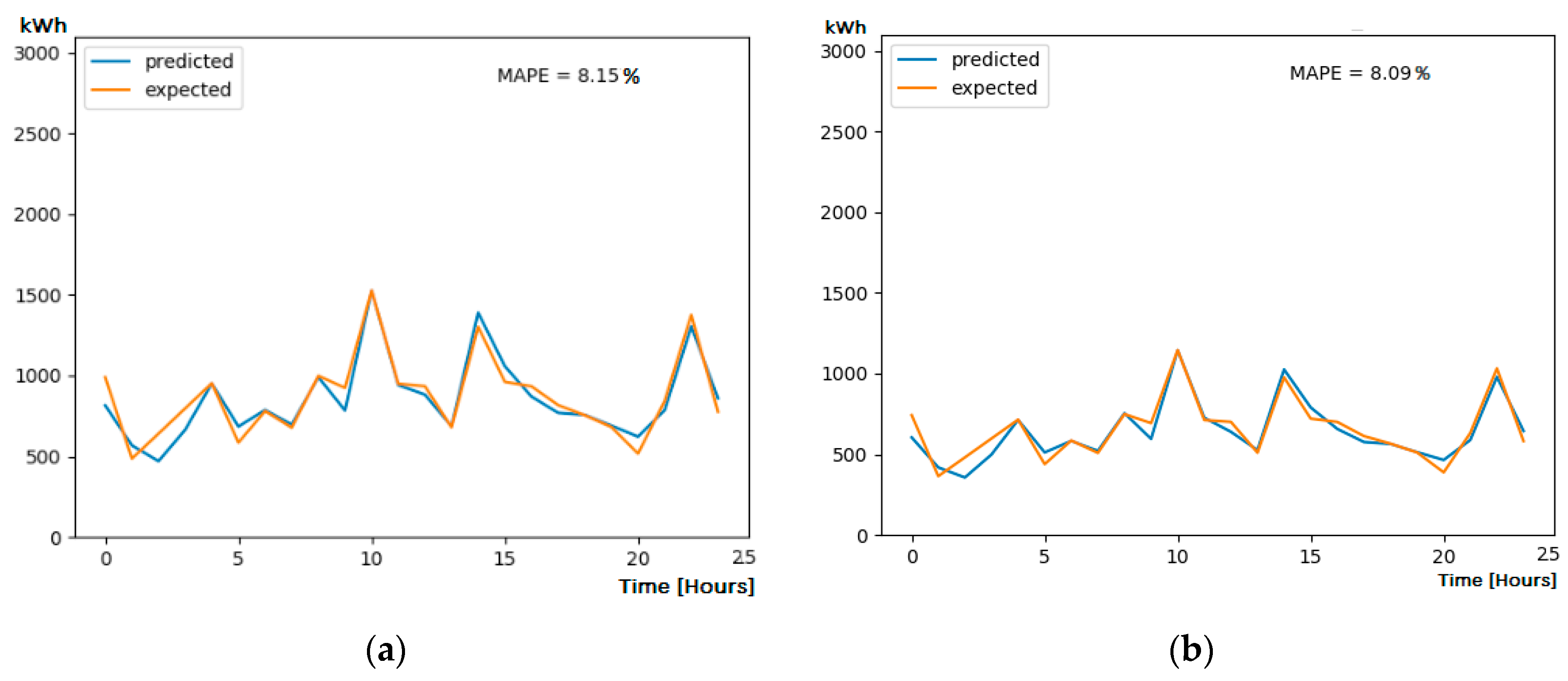
The ensemble predictor that uses the genetic algorithm-based approach to generate specific weights for all the time stamps of the forecasting window achieves a better MAPE (see Figure 12) compared to the individual predictors (i.e., 8.15% for IT servers, respectively 8.09% for cooling sub-system).
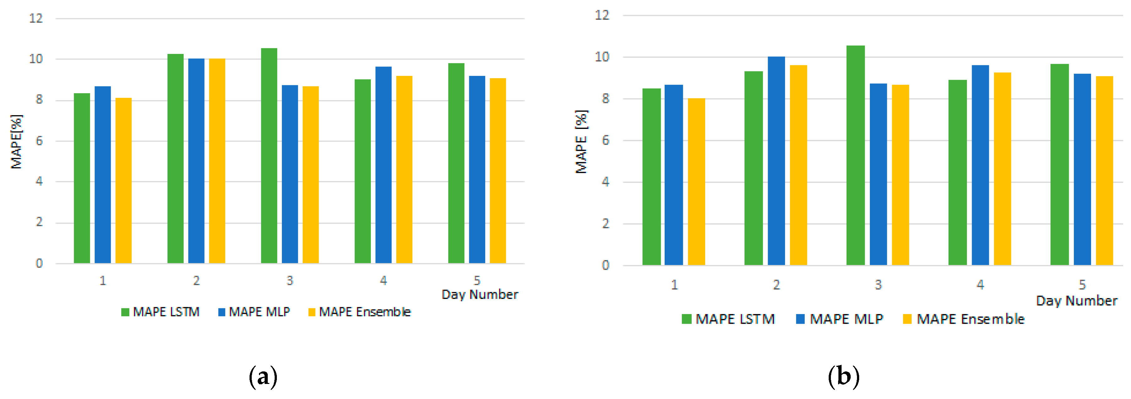
Figure 13 shows the average MAPE obtained by the two individual prediction models LSTM and MLP as well as the ensemble model over the entire testing period for the day-ahead time frame. The LSTM models MAPE average is 9.50%, MLP achieves a MAPE of 9.276%, while the ensemble models achieve a MAPE of 9%. As it can be seen in the chart, on some days the LSTM works better, while on others the MLP models predict with better accuracy. On the second test day, the ensemble model achieves a MAPE of 8.15%, best result obtained by any of the three models.
The second set of experiments aims to evaluate the enhancement bought by the intra-day forecasting process considering not just the forecasting errors but also the difference between the forecasted energy values by the day-ahead and intra-day predictions and the actual monitored values. This represents an important measure of the prediction efficiency as the deviation between the forecasted values on the two horizons; the real monitored values are translated in an uncertainty and a cost in the delivery of flexibility services in the DR programs.
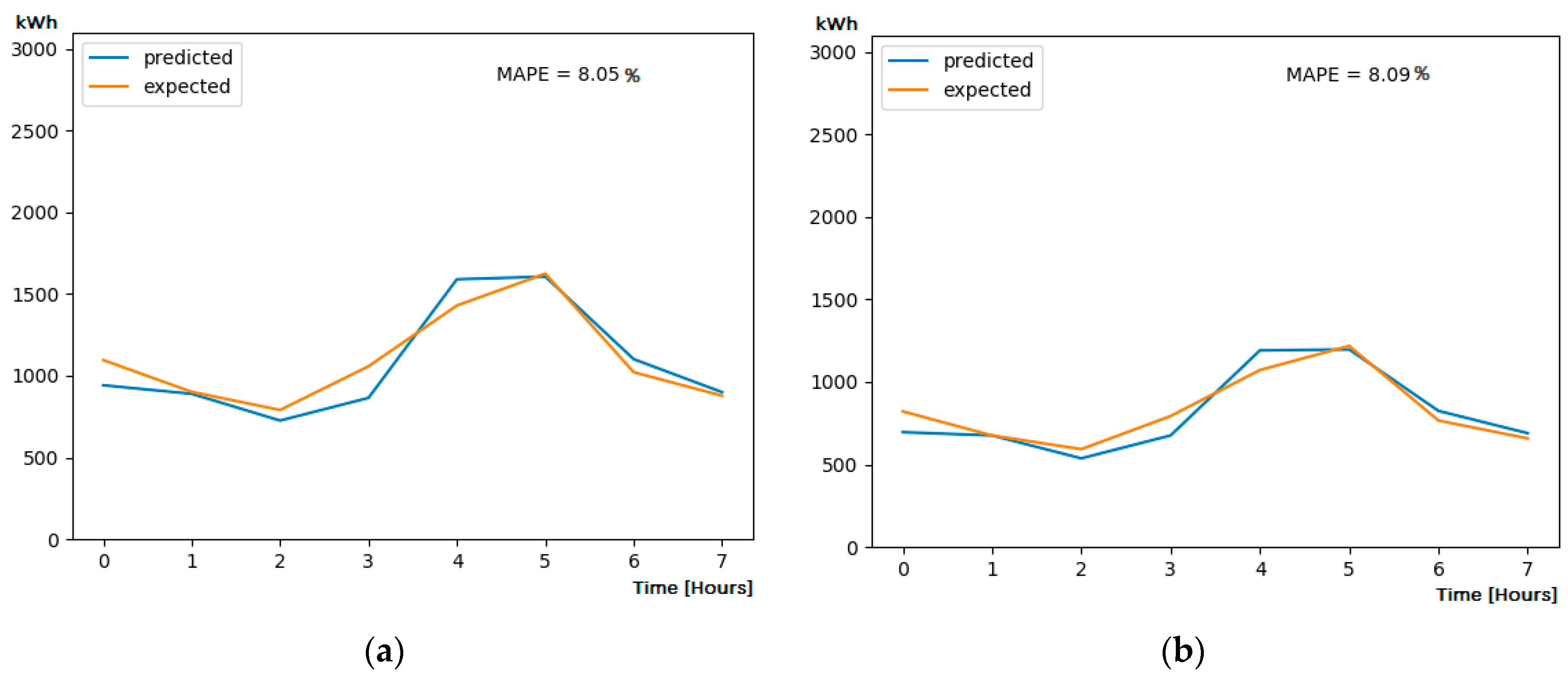
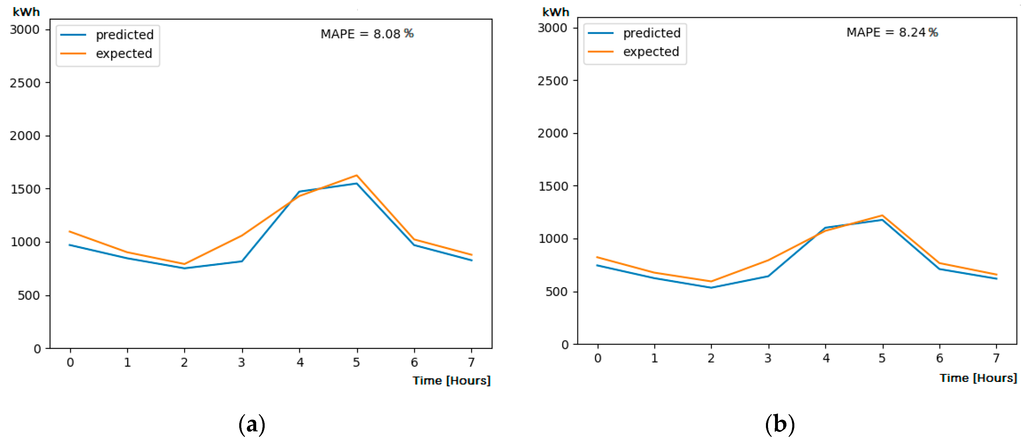
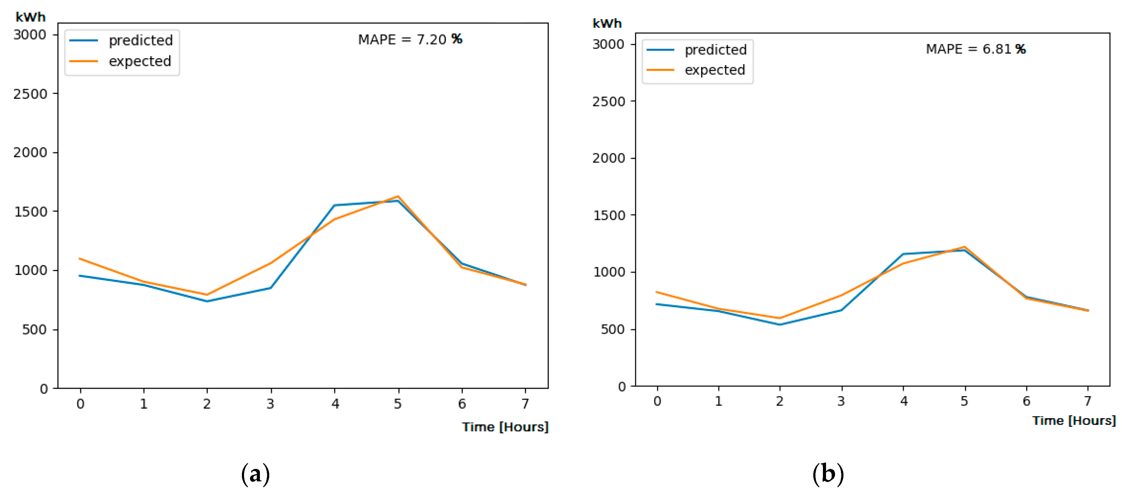
As it can be seen from Figure 14, Figure 15 and Figure 16, the prediction models on the intra-day forecasting outperform the day-ahead prediction results. At the same time, the ensemble predictor also gives the best results on the intra-day time window achieving a MAPE of 7% on average taking the server room and cooling sub-system components.
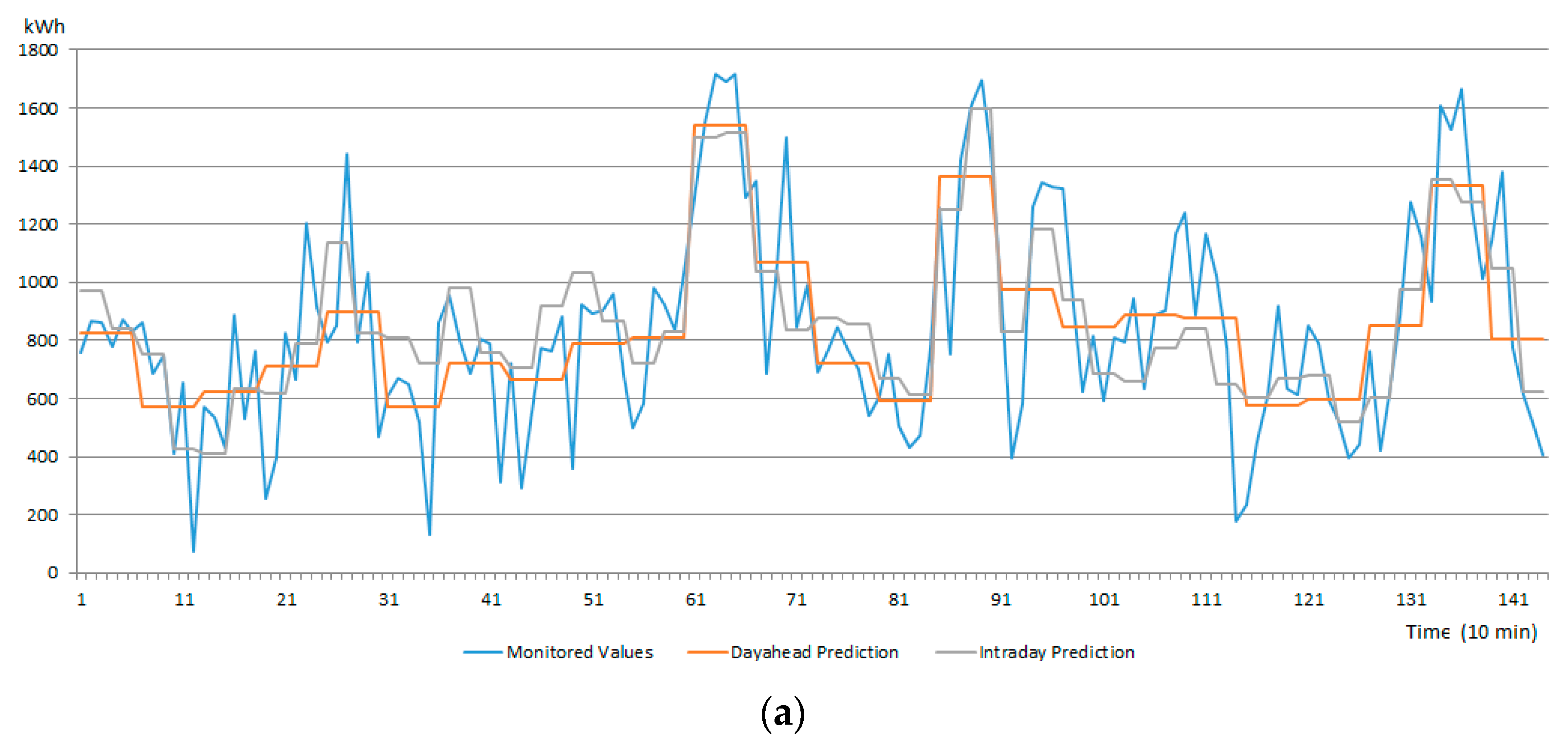
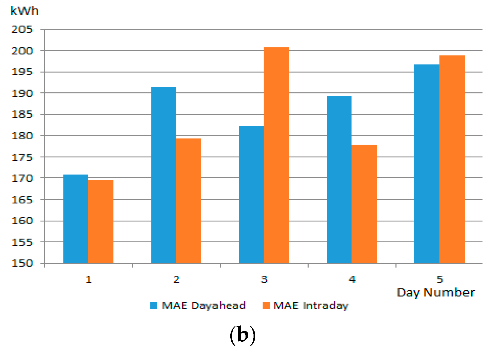
Furthermore, we have evaluated the deviation between the actual energy monitored values and the ones forecasted by the intra-day and day-ahead processes over the test data. We have computed the mean absolute error (MAE) value with respect to the actual values at a 10-min granularity. The intra-day prediction gives better results in terms of total energy estimation in 3 out the 5 test days, achieving estimations with more than 600 kWh of energy daily better in respect to the day-ahead process. Overall the 5 test days, the intra-day prediction total energy prediction improvement compared with the day-ahead one is of about 100 kWh.
Figure 17 shows the predictions for day-ahead and intra-day models plotted against the actual monitored data at a 10-min sampling rate over the 4th day of test data. During this test day, the MAE between the day-ahead forecast result and the monitored data is 191.42, while the MAE between the intra-day and the monitored data is 179.42, meaning that on average, the prediction is better with about 277 kWh of energy. Table 3 presents the prediction results for electrical energy consumption of the IT servers and cooling sub-system for the considered DC.
4.2. DC Flexibility Forecasting Results
For predicting the DC energy flexibility, we have divided the forecasting problem into two sub-problems namely the prediction of the above-baseline flexibility curve and the prediction of the below-baseline flexibility curve. For this purpose, the initial training data have been split according to the computed baseline into two training datasets containing the decomposition of the training curve into below and above differences with respect to the calculated DC baseline. Each flexibility ensemble model trains two neural networks, namely MLP and LSTM, ensembled using the genetic heuristic.
To train each MLP neural network within each flexibility forecasting model, a dataset consisting of <input, output> pairs was used. The IT servers’ sub-system flexibility prediction model was trained first and then the output was used to train the cooling system flexibility prediction model. Table 4 shows the input and outputs for the two neural networks composing the server room flexibility model, and the two neural networks composing the cooling system flexibility model. The neural networks were trained using a k-fold technique, using 100 epochs.
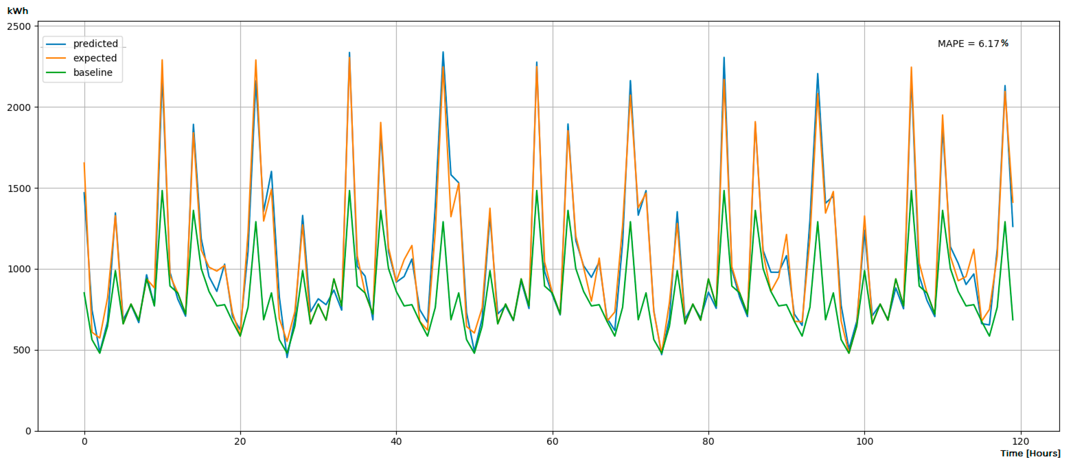
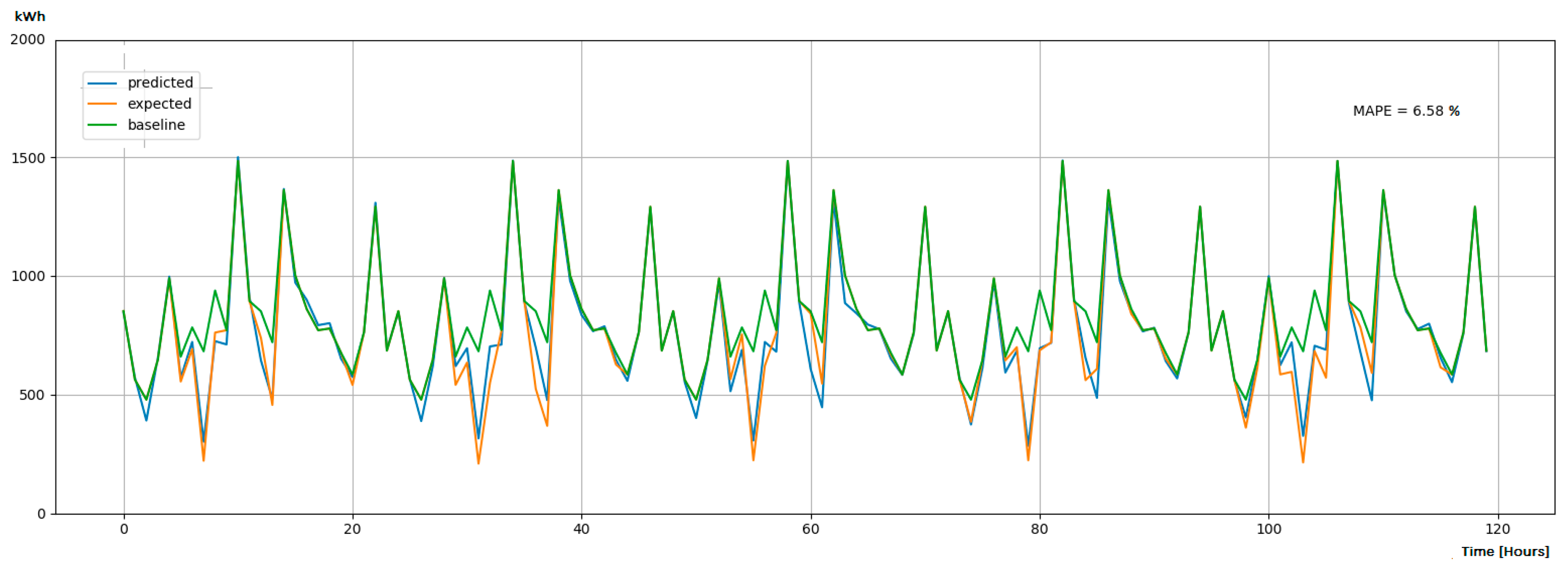
The flexibility forecasting techniques were evaluated to predict the energy flexibility above and below curves for the 4 days of test data. Figure 18 shows the results obtained for assessing the flexibility above the baseline over the test period. The prediction has a 6.17% MAPE, the predicted values (colored in blue) following closely the real values (colored in orange). The baseline is depicted in green. Furthermore, Figure 19 depicts the below flexibility, the prediction exhibiting a MAPE of 6.58%. The average MAPE of the day-ahead flexibility prediction is of 6.37%.
5. Conclusions
In this paper we have proposed an ensemble-based energy prediction model to forecast DCs energy demand and flexibility aiming to enable their safe participation to DR programs. The selection of the short-term time horizon (i.e., day-ahead and intra-day), energy flavors considered as well as of the main DC sub-systems modeled as flexible assets where driven by the nowadays DR programs characteristics. The implemented ensemble-based DC energy prediction model is based on a set of individual neural network weak learners while a genetic heuristic is used to determine the optimal combination of the outcome of individual predictors to minimize the prediction error. The results are promising as the model is feasible to be used for engaging DCs in DR programs. In the case of DC energy demand forecasting results, the ensemble prediction obtained the best MAPE values compared to individual predictors such as MLP and LSTM, 8.15% for the day-ahead time frame. The intra-day predictors manage to improve the results generated by the day-ahead ones (7.2% MAPE) while for flexibility forecasting 6.37% average MAPE was obtained for the below and above the baseline curves.
As for future work, we plan to investigate how the prediction model could be potentially decentralized to run closer to the edge (i.e., consumption point) and how it could work in conjunction with Big Data technologies for allowing the integration of large-scale distributed streams of energy data generated by the IoT power meters and by a significant number of smart grid prosumers. At the same time, other non-energy related features (i.e., holiday) or social features will be considered to improve the prediction of energy related behavior and we plan to test the proposed approach in the context of H2020 CATALYST pilot DCs: the Poznan Supercomputing and Networking Center HPC and Engineering SPA colocation DC from Pont Saint Martin.
Author Contributions
Conceptualization, T.C. and I.A.; Methodology, T.C. and A.V.V.; Software, A.V.V. and M.A.; Validation, C.P. and A.V.V.; Formal Analysis, M.A.; Investigation, B.I.; Data Curation, C.P.; Writing—Original Draft Preparation, T.C., A.V.V. and I.S.; Writing-Review & Editing, I.A. and V.T.D.; Visualization, B.I.; Supervision, I.S. and V.T.D. All authors have read and agreed to the published version of the manuscript.
Funding
This research was funded by the European Union’s Horizon 2020 research and innovation programme grant number 768739 (H2020 CATALYST) and grant number 774478 (H2020 eDREAM). The APC was funded by the Technical University of Cluj-Napoca through the grants for scientific research support programme, grant number L2GA6-13-14/2019.
Koronen, C.; Ahman, M.; Nilsson, L.J. Data centres in future European energy systems—Energy efficiency, integration and policy. Energy Effic. J.2020, 13, 129–144. [Google Scholar] [CrossRef]
Cioara, T.; Anghel, I.; Bertoncini, M.; Salomie, I.; Arnone, D.; Mammina, M.; Velivassaki, T.; Antal, M. Optimized flexibility management enacting Data Centres participation in Smart Demand Response programs. Future Gener. Comput. Syst.2018, 78, 330–342. [Google Scholar] [CrossRef]
Huang, P.; Copertaro, B.; Zhang, X.; Shen, J.; Lofgren, I.; Ronnelid, M.; Fahlen, J.; Andersson, D.; Svanfeldt, M. A review of data centers as prosumers in district energy systems: Renewable energy integration and waste heat reuse for district heating. Appl. Energy2020, 258, 114109. [Google Scholar] [CrossRef]
Alapera, I.; Honkapuro, S.; Paananen, J. Data centers as a source of dynamic flexibility in smart girds. Appl. Energy2018, 229, 69–79. [Google Scholar] [CrossRef]
Ponnaganti, P.; Pillai, J.R.; Bak-Jensen, B. Opportunities and challenges of demand response in active distribution networks. WIREs Energy Environ.2018, 7, e271. [Google Scholar] [CrossRef]
Cioara, T.; Anghel, I.; Antal, M.; Crisan, S.; Salomie, I. Data center optimization methodology to maximize the usage of locally produced renewable energy. In Proceedings of the 2015 Sustainable Internet and ICT for Sustainability (SustainIT), Madrid, Spain, 14–15 April 2015; pp. 1–8. [Google Scholar] [CrossRef]
Ogedengbe, E.O.B.; Aderoju, P.A.; Nkwaze, D.C.; Aruwajoye, J.B.; Shitta, M.B. Optimization of energy performance with renewable energy project sizing using multiple objective functions. Energy Rep.2019, 5, 898–908. [Google Scholar] [CrossRef]
Cioara, T.; Anghel, I.; Salomie, I.; Antal, M.; Pop, C.; Bertoncini, M.; Arnone, D.; Pop, F. Exploiting data centres energy flexibility in smart cities: Business scenarios. Inf. Sci.2019, 476, 392–412. [Google Scholar] [CrossRef]
Feuerriegel, S.; Neumann, D. Integration scenarios of Demand Response into electricity markets: Load shifting, financial savings and policy implications. Energy Policy2016, 96, 231–240. [Google Scholar] [CrossRef]
Nicholas Good, K.; Ellis, P.M. Review and classification of barriers and enablers of demand response in the smart grid. Renew. Sustain. Energy Rev.2017, 72, 57–72. [Google Scholar] [CrossRef]
Fallah, S.N.; Deo, R.C.; Shojafar, M.; Conti, M.; Shamshirband, S. Computational Intelligence Approaches for Energy Load Forecasting in Smart Energy Management Grids: State of the Art, Future Challenges, and Research Directions. Energies2018, 11, 596. [Google Scholar] [CrossRef]
Wang, Y.; Chen, Q.; Hong, T.; Kang, C. Review of smart meter data analytics: Applications, methodologies, and challenges. IEEE Trans. Smart Grid2018, 10, 3125–3148. [Google Scholar] [CrossRef]
Zhang, X.; Li, Z.; Ma, L.; Chong, C.; Ni, W. Forecasting the Energy Embodied in Construction Services Based on a Combination of Static and Dynamic Hybrid Input-Output Models. Energies2019, 12, 300. [Google Scholar] [CrossRef]
Miyuru, D.; Wen, Y.; Fan, R. Data center energy consumption modeling: A survey. IEEE Commun. Surv. Tutor.2015, 18, 732–794. [Google Scholar]
Jim, G. Machine Learning Applications for Data Center Optimization. 2014. Available online: https://ai.google/research/pubs/pub42542 (accessed on 15 December 2019).
Tseng, F.; Wang, X.; Chou, L.; Chao, H.; Leung, V.C.M. Dynamic Resource Prediction and Allocation for Cloud Data Center Using the Multiobjective Genetic Algorithm. IEEE Syst. J.2018, 12, 1688–1699. [Google Scholar] [CrossRef]
Li, Y.; Hu, H.; Wen, Y.; Zhang, J. Learning-based power prediction for data centre operations via deep neural networks. In Proceedings of the 5th International Workshop on Energy Efficient Data Centres (E2DC ’16), Waterloo, ON, Canada, 21 June 2016; ACM: New York, NY, USA, 2016; p. 10. [Google Scholar] [CrossRef]
Grange, L.; da Costa, G.; Stolf, P. Green IT scheduling for data center powered with renewable energy. Future Gener. Comput. Syst.2018, 86, 99–120. [Google Scholar] [CrossRef]
Ferreira, J.; Callou, G.; Josua, A.; Tutsch, D.; Maciel, P. An Artificial Neural Network Approach to Forecast the Environmental Impact of Data Centers. Information2019, 10, 113. [Google Scholar] [CrossRef]
Antal, M.; Cioara, T.; Anghel, I.; Pop, C.; Salomie, I. Transforming Data Centers in Active Thermal Energy Players in Nearby Neighborhoods. Sustainability2018, 10, 939. [Google Scholar] [CrossRef]
Makridakis, S.; Spiliotis, E.; Assimakopoulos, V. Statistical and Machine Learning forecasting methods: Concerns and ways forward. PLoS ONE2018, 13, e0194889. [Google Scholar] [CrossRef]
Marino, D.L.; Amarasinghe, K.; Manic, M. Building energy load forecasting using Deep Neural Networks. In Proceedings of the IECON 2016—42nd Annual Conference of the IEEE Industrial Electronics Society, Florence, Italy, 23–26 October 2016; pp. 7046–7051. [Google Scholar]
Cheng, Y.; Xu, C.; Mashima, D.; Thing, V.L.; Wu, Y. PowerLSTM: Power demand forecasting using long short-term memory neural network. In Proceedings of the International Conference on Advanced Data Mining and Applications, Singapore, 5–6 November 2017; Springer: Cham, Switzerland, 2017; pp. 727–740. [Google Scholar]
Mocanu, E.; Nguyen, P.H.; Gibescu, M.; Kling, W.L. Deep learning for estimating building energy consumption Sustainable Energy. Grids Netw.2016, 6, 91–99. [Google Scholar]
Fayaz, M.; Kim, D. A Prediction Methodology of Energy Consumption Based on Deep Extreme Learning Machine and Comparative Analysis in Residential Buildings. Electronics2018, 7, 222. [Google Scholar] [CrossRef]
Liang, Y.; Niu, D.; Hong, W.C. Short term load forecasting based on feature extraction and improved general regression neural network model. Energy2019, 166, 653–663. [Google Scholar] [CrossRef]
Rahman, H.; Selvarasan, I.; Begum, J. Short-Term Forecasting of Total Energy Consumption for India-A Black Box Based Approach. Energies2018, 11, 3442. [Google Scholar] [CrossRef]
Zufferey, T.; Ulbig, A.; Koch, S.; Hug, G. Forecasting of Smart Meter Time Series Based on Neural Networks. Lect. Notes Comput. Sci.2017, 10097, 10–21. [Google Scholar] [CrossRef]
Lee, S.; Jung, S.; Lee, J. Prediction Model Based on an Artificial Neural Network for User-Based Building Energy Consumption in South Korea. Energies2019, 12, 608. [Google Scholar] [CrossRef]
Huang, C.-J.; Kuo, P.-H. A Short-Term Wind Speed Forecasting Model by Using Artificial Neural Networks with Stochastic Optimization for Renewable Energy Systems. Energies2018, 11, 2777. [Google Scholar] [CrossRef]
Kampelis, N.; Tsekeri, E.; Kolokotsa, D.; Kalaitzakis, K.; Isidori, D.; Cristalli, C. Development of Demand Response Energy Management Optimization at Building and District Levels Using Genetic Algorithm and Artificial Neural Network Modelling Power Predictions. Energies2018, 11, 3012. [Google Scholar] [CrossRef]
Fan, C.; Sun, Y.; Zhao, Y.; Song, M.; Wang, J. Deep learning-based feature engineering methods for improved building energy prediction. Appl. Energy2019, 240, 35–45. [Google Scholar] [CrossRef]
Chen, K.; He, Z.; Wang, S.X. Learning-based Data Analytics: Moving Towards Transparent Power Grids. Csee J. Power Energy Syst.2018, 4, 67–82. [Google Scholar] [CrossRef]
Chen, Y.; Tan, H. Short-term prediction of electric demand in building sector via hybrid support vector regression. Appl. Energy2017, 204, 1363–1374. [Google Scholar] [CrossRef]
Kim, M.; Choi, W.; Jeon, Y.; Liu, L. A Hybrid Neural Network Model for Power Demand Forecasting. Energies2019, 12, 931. [Google Scholar] [CrossRef]
Kuo, P.-H.; Huang, C.-J. An Electricity Price Forecasting Model by Hybrid Structured Deep Neural Networks. Sustainability2018, 10, 1280. [Google Scholar] [CrossRef]
Zahid, M.; Ahmed, F.; Javaid, N.; Abbasi, R.A.; Zainab Kazmi, H.S.; Javaid, A.; Bilal, M.; Akbar, M.; Ilahi, M. Electricity Price and Load Forecasting using Enhanced Convolutional Neural Network and Enhanced Support Vector Regression in Smart Grids. Electronics2019, 8, 122. [Google Scholar] [CrossRef]
He, W. Load Forecasting via Deep Neural Networks. Procedia Comput. Sci.2017, 122, 308–314. [Google Scholar] [CrossRef]
Kim, T.Y.; Cho, S.B. Predicting the Household Power Consumption Using CNN-LSTM Hybrid Networks. In Proceedings of the International Conference on Intelligent Data Engineering and Automated Learning—IDEAL 2018, Madrid, Spain, 21–23 November 2018; pp. 481–490. [Google Scholar]
Bouktif, S.; Fiaz, A.; Ouni, A.; Serhani, M.A. Optimal Deep Learning LSTM Model for Electric Load Forecasting using Feature Selection and Genetic Algorithm: Comparison with Machine Learning Approaches. Energies2018, 11, 1636. [Google Scholar] [CrossRef]
Eseye, A.T.; Zhang, J.; Zheng, D. Short-term photovoltaic solar power forecasting using a hybrid wavelet-PSO- SVM model based on SCADA and meteorological information. Renew. Energy2017, 118, 357–367. [Google Scholar]
Nayab, A.; Ashfaq, T.; Aimal, S.; Rasool, A.; Javaid, N.; Khan, Z.A. Load and Price Forecasting in Smart Grids Using Enhanced Support Vector Machine. In Advances in Internet, Data and Web Technologies. EIDWT 2019. Lecture Notes on Data Engineering and Communications Technologies; Barolli, L., Xhafa, F., Khan, Z., Odhabi, H., Eds.; Springer: Cham, Switzerland, 2019; Volume 29. [Google Scholar]
Ouyang, T.; He, Y.; Li, H.; Sun, Z.; Baek, S. A Deep Learning Framework for Short-term Power Load Forecasting. Comput. Eng. Financ. Sci.2017. [Google Scholar]
Fu, C.; Li, G.-Q.; Lin, K.-P.; Zhang, H.-J. Short-Term Wind Power Prediction Based on Improved Chicken Algorithm Optimization Support Vector Machine. Sustainability2019, 11, 512. [Google Scholar] [CrossRef]
Data-Driven Baseline Estimation of Residential Buildings for Demand Response. Available online: https://www.mdpi.com/1996-1073/8/9/10239 (accessed on 15 December 2019).
Wang, C.; Urgaonkar, B.; Wang, Q.; Kesidis, G.; Sivasubramaniam, A. Data Center Power Cost Optimization via Workload Modulation. In Proceedings of the 2013 IEEE/ACM 6th International Conference on Utility and Cloud Computing, Dresden, Germany, 9–12 December 2013. [Google Scholar]
Rynkiewicz, J. Asymptotic statistics for multilayer perceptron with ReLU hidden units. Neurocomputing2019, 342, 16–23. [Google Scholar] [CrossRef]
Le, X.-H.; Ho, H.V.; Lee, G.; Jung, S. Application of Long Short-Term Memory (LSTM) Neural Network for Flood Forecasting. Water2019, 11, 1387. [Google Scholar] [CrossRef]
Figure 1.
DC participation in DR programs scenario.
Figure 1.
DC participation in DR programs scenario.
Figure 2.
DC ensemble-based energy forecasting model.
Figure 2.
DC ensemble-based energy forecasting model.
Figure 3.
IT Servers and Cooling sub-systems relation modelling.
Figure 3.
IT Servers and Cooling sub-systems relation modelling.
Figure 4.
Individual neural network predictor model for DC energy sub-systems.
Figure 4.
Individual neural network predictor model for DC energy sub-systems.
Figure 5.
Time frames used to forecast DC energy for DR programs enrolment.
Figure 5.
Time frames used to forecast DC energy for DR programs enrolment.
Figure 6.
Features used for DC energy flexibility prediction.
Figure 6.
Features used for DC energy flexibility prediction.
Figure 7.
Electrical energy flexibility forecasting model.
Figure 7.
Electrical energy flexibility forecasting model.
Figure 8.
Genetic algorithm for weighted ensemble determination.
Figure 8.
Genetic algorithm for weighted ensemble determination.
Figure 9.
Electrical energy historical data used in forecasting (orange—cooling sub-system & blue—IT servers’ sub-system).
Figure 9.
Electrical energy historical data used in forecasting (orange—cooling sub-system & blue—IT servers’ sub-system).
Figure 10.
Day-ahead energy demand predictions using MLP: (a) IT servers and (b) cooling sub-systems.
Figure 10.
Day-ahead energy demand predictions using MLP: (a) IT servers and (b) cooling sub-systems.
Figure 11.
Day-ahead energy demand predictions using LSTM: (a) IT servers and (b) cooling sub-systems.
Figure 11.
Day-ahead energy demand predictions using LSTM: (a) IT servers and (b) cooling sub-systems.
Figure 12.
Day-ahead electrical energy demand predictions using ensemble model: (a) IT servers and (b) cooling sub-systems.
Figure 12.
Day-ahead electrical energy demand predictions using ensemble model: (a) IT servers and (b) cooling sub-systems.
Figure 13.
Average MAPE values different prediction model configurations: (a) IT servers and (b) cooling sub-systems.
Figure 13.
Average MAPE values different prediction model configurations: (a) IT servers and (b) cooling sub-systems.
Figure 14.
Intra-day electrical energy demand predictions using MLP model: (a) IT servers and (b) cooling sub-systems.
Figure 14.
Intra-day electrical energy demand predictions using MLP model: (a) IT servers and (b) cooling sub-systems.
Figure 15.
Intra-day electrical energy demand predictions using LSTM model: (a) IT servers and (b) cooling sub-system.
Figure 15.
Intra-day electrical energy demand predictions using LSTM model: (a) IT servers and (b) cooling sub-system.
Figure 16.
Intra-day electrical energy demand predictions using ensemble model: (a) IT servers and (b) cooling sub-system.
Figure 16.
Intra-day electrical energy demand predictions using ensemble model: (a) IT servers and (b) cooling sub-system.
Figure 17.
Day-ahead and intra-day energy demand prediction results vs. actual monitored values ((a)—detailed results day number 4, (b)—MAE distribution on 5 days of testing data).
Figure 17.
Day-ahead and intra-day energy demand prediction results vs. actual monitored values ((a)—detailed results day number 4, (b)—MAE distribution on 5 days of testing data).
Figure 18.
Day-ahead energy flexibility above baseline prediction.
Figure 18.
Day-ahead energy flexibility above baseline prediction.
Figure 19.
Day-ahead energy flexibility below the baseline prediction.
Figure 19.
Day-ahead energy flexibility below the baseline prediction.
Table 1.
Characteristics of the test bed DC.
Table 1.
Characteristics of the test bed DC.
Sub-System
Characteristics
Cooling system
IT servers
Table 2.
Prediction models configurations for IT Servers and Cooling DC sub-systems.
Table 2.
Prediction models configurations for IT Servers and Cooling DC sub-systems.
DC Component
Time Frame
Prediction Model
No. Models
Contextual Features
No. Inputs
No. Neurons on Hidden Layer
No. Outputs
IT servers consumption
Day-ahead
MLP
1
isWeekend
25
37
24
LSTM
1
isWeekend
25
47
24
Intra-day
MLP
6
partOfDay
9
20
8
LSTM
6
partOfDay
9
16
8
Cooling consumption
Day-ahead
MLP
1
isWeekend
25
37
24
LSTM
1
isWeekend
25
47
24
Intra-day
MLP
6
partOfDay
9
20
8
LSTM
6
partOfDay
9
16
8
Table 3.
DC energy demand prediction results.
Table 3.
DC energy demand prediction results.
Prediction Model
Time Frame
Best MAPE Value [%]
IT Servers Sub-System
Cooling Sub-System
MLP
Day-ahead
8.68
8.68
Intra-day
8.05
8.09
LSTM
Day-ahead
8.37
8.50
Intra-day
8.08
8.24
Ensemble
Day-ahead
8.15
8.09
Intra-day
7.20
6.81
Table 4.
Features used for ensemble-based flexibility prediction.
Table 4.
Features used for ensemble-based flexibility prediction.
DC Sub-System
Prediction Type
Input Features
N
M
IT servers
Day-ahead
Historical load Historical baseline Current baseline Contextual features
24
24
77
100
5
24
Cooling system
Day-ahead
Historical load Historical baseline Current baseline Contextual features Server room flexibility
Vesa, A.V.; Cioara, T.; Anghel, I.; Antal, M.; Pop, C.; Iancu, B.; Salomie, I.; Dadarlat, V.T.
Energy Flexibility Prediction for Data Center Engagement in Demand Response Programs. Sustainability2020, 12, 1417.
https://doi.org/10.3390/su12041417
AMA Style
Vesa AV, Cioara T, Anghel I, Antal M, Pop C, Iancu B, Salomie I, Dadarlat VT.
Energy Flexibility Prediction for Data Center Engagement in Demand Response Programs. Sustainability. 2020; 12(4):1417.
https://doi.org/10.3390/su12041417
Chicago/Turabian Style
Vesa, Andreea Valeria, Tudor Cioara, Ionut Anghel, Marcel Antal, Claudia Pop, Bogdan Iancu, Ioan Salomie, and Vasile Teodor Dadarlat.
2020. "Energy Flexibility Prediction for Data Center Engagement in Demand Response Programs" Sustainability 12, no. 4: 1417.
https://doi.org/10.3390/su12041417
APA Style
Vesa, A. V., Cioara, T., Anghel, I., Antal, M., Pop, C., Iancu, B., Salomie, I., & Dadarlat, V. T.
(2020). Energy Flexibility Prediction for Data Center Engagement in Demand Response Programs. Sustainability, 12(4), 1417.
https://doi.org/10.3390/su12041417
Note that from the first issue of 2016, this journal uses article numbers instead of page numbers. See further details here.
Article Metrics
No
No
Article Access Statistics
For more information on the journal statistics, click here.
Multiple requests from the same IP address are counted as one view.
Vesa, A.V.; Cioara, T.; Anghel, I.; Antal, M.; Pop, C.; Iancu, B.; Salomie, I.; Dadarlat, V.T.
Energy Flexibility Prediction for Data Center Engagement in Demand Response Programs. Sustainability2020, 12, 1417.
https://doi.org/10.3390/su12041417
AMA Style
Vesa AV, Cioara T, Anghel I, Antal M, Pop C, Iancu B, Salomie I, Dadarlat VT.
Energy Flexibility Prediction for Data Center Engagement in Demand Response Programs. Sustainability. 2020; 12(4):1417.
https://doi.org/10.3390/su12041417
Chicago/Turabian Style
Vesa, Andreea Valeria, Tudor Cioara, Ionut Anghel, Marcel Antal, Claudia Pop, Bogdan Iancu, Ioan Salomie, and Vasile Teodor Dadarlat.
2020. "Energy Flexibility Prediction for Data Center Engagement in Demand Response Programs" Sustainability 12, no. 4: 1417.
https://doi.org/10.3390/su12041417
APA Style
Vesa, A. V., Cioara, T., Anghel, I., Antal, M., Pop, C., Iancu, B., Salomie, I., & Dadarlat, V. T.
(2020). Energy Flexibility Prediction for Data Center Engagement in Demand Response Programs. Sustainability, 12(4), 1417.
https://doi.org/10.3390/su12041417
Note that from the first issue of 2016, this journal uses article numbers instead of page numbers. See further details here.

 ,
, 


.jpeg)


