Spatiotemporal Characteristics of Bike-Sharing Usage around Rail Transit Stations: Evidence from Beijing, China

Abstract

As an emerging mode of transport, bike-sharing is being quickly accepted by Chinese residents due to its convenience and environmental friendliness. As hotspots for bike-sharing, railway-station service areas attract thousands of bikes during peak hours, which can block roads and pedestrian walkways. Of the many works devoted to the connection between bikes and rail, few have addressed the spatial‒temporal pattern of bike-sharing accumulating around station service areas. In this work, we investigate the distribution patterns of bike-sharing in station service areas, which are influenced not only by railway-station ridership but also by the built environment around the station, illustrating obvious spatial heterogeneity. To this end, we established a geographic weighted regression (GWR) model to capture this feature considering the variables of passenger flow and the built environment. Using the data from bike-sharing in Beijing, China, we applied the GWR model to carry out a spatiotemporal characteristic analysis of the relationship between bike-sharing usage in railway-station service areas and its determinants, including the passenger flow in stations, land use, bus lines, and road-network characteristics. The influence of these factors on bike-sharing usage is quite different in time and space. For instance, bus lines are a competing mode of transport with bike-sharing in suburban areas but not in city centers, whereas industrial and residential areas could also heavily affect the bike-sharing demand as well as railway-station ridership. The results of this work can help facilitate the dynamic allocation of bike-sharing and increase the efficiency of this emerging mode of transport.

1. Introduction

In recent years, bike-sharing has grown significantly in many Chinese cities, as it caters to the public transport policies of convenience, sustainability, and energy saving [1,2]. Essentially, bike-sharing is an oriented production-service system (PSS), whereby the ownership of bicycles is retained by providers (e.g., Ofo, Mobike, 99bicycle, and Wisdom-Enjoyed Cycling) who sell the functions of the bikes. Bike-sharing has benefits for short-distance travel and connecting “the last kilometer” in a given city [3], which is especially evident in the vicinity of rail transit stations. Bike-sharing is a convenient way for residents to travel, but it also suffers from some shortcomings, such as unreasonable bicycle parking and the failure to transfer bikes in time. Thus, a better understanding of the spatiotemporal characteristics of bike-sharing is needed and could provide management and operational support for enterprises and government departments [4,5,6]. Station service areas are especially interesting for their unique characteristics that affect bike-sharing usage.

Studies on bike-sharing mainly focus on demand forecasting [7,8,9,10], pricing schemes [11,12,13], bike-sharing systems (BSS) [3,14,15], and spatiotemporal characteristics [16,17,18]. Demand forecasting, the preliminary work of bike-sharing, determines the number of shared bikes to some extent. Bike-sharing operation costs comprise the system operation, administration, marketing, and utility costs associated with hardwired stations. Pricing schemes are directly related to passenger flow and operation [11]. Bike-sharing systems (BSS) are a topic worth studying, especially in terms of user satisfaction [19], bike-sharing services [20], rebalancing operations [21], and the like. Compared with demand forecasting, pricing schemes, and BSS, the spatiotemporal characteristics of bike-sharing usage are fundamental to understand the operation and management of bike-sharing services. While analyzing the interaction between bike-sharing and rail transit, we may also explore the influence of land-use attributes on bike-sharing usage in terms of transit-oriented development (TOD).

The passenger flow [1] and built environment [22] are important influences on the spatiotemporal characteristics of bike-sharing usage. The greater the passenger flow, the more shared bikes are used; however, the effects of passenger-flow volume have been rarely studied even though user attributes, travel characteristics, and user preferences have been frequently analyzed. Analysis of the user attributes (gender, age, income, car ownership, etc.) related to bike-sharing was necessary to understand travel demands and improve customer satisfaction [23]. The travel characteristics (travel time, travel distance, travel purpose, etc.) of bike-sharing are of great importance in terms of demand forecasting and the planning of bike-sharing operations. Giving full consideration to user preferences could effectively increase operation costs.

In regard to the built environment, Tran et al. analyzed the factors influencing the usage flow of a bike-sharing system in Lyon, France, and found that the network density of bike-sharing and the station capacity were plausibly correlated to the bike-sharing usage [24]. Mateo-Babiano et al. analyzed Brisbane’s CityCycle scheme in Australia [25]. Inner-city stations near to off-road infrastructure saw the most active bike-sharing usage, with CityCycle more heavily used on weekends for recreational purposes. From the survey data of 90 randomly selected residents, the bicycle fare, existence of separated bicycle lane, bicycle quality, pavement quality, proximity of bicycle stations to bus stops, bicycle training programs, and gender and employment statuses of the respondents significantly influenced public preferences regarding BSS in Mashhad [26]. Bike-sharing linked to the bus rapid transit system played an important role, and minor changes could improve their multimodality [27]. Bike-sharing affected the built transportation system [27]. However, the built transportation system also affected bike-sharing usage. Wang et al. analyzed the effects of nearby businesses and jobs on trips to and from stations using bike-sharing [28]. Bike-sharing programs were, theoretically, best suited to locations with higher population densities and more destinations that could be easily accessed. Built-environment variables, including station attributes and accessibility, cycling infrastructure, public transport facilities, and land-use characteristics, were all considered in analyzing the spatial correlations of bike-sharing usage between nearby stations [29].

Clearly, few previous studies have analyzed the spatiotemporal characteristics of bike-sharing usage in terms of passenger flow and the built environment. Rail transit stations are an important part of urban transportation, and the unique characteristics of their service areas impact on bike-sharing usage. This paper aims to analyze the spatiotemporal characteristics of bike-sharing usage around rail transit stations using data from Beijing, China. Specifically, the contributions of this work can be summarized as follows: (i) on the basis of analysis of the influencing factors, a geographic weighted regression (GWR) model is built to capture the particular spatiotemporal characteristics of bike-sharing usage around rail transit stations considering the variables of passenger flow and the built environment; (ii) referring to bike-sharing in Beijing, China as a case study, we analyze the influence of the passenger flow into and out of the stations, land use, bus lines, and road-network characteristics on the bike-sharing usage in terms of time and space.

The remainder of this paper comprises the following: Section 2 gives the data description; Section 3 describes the analysis methodology; Section 4 we give the model effectiveness analysis, and the influence of the passenger flow, land use, bus lines and road-network characteristics on the bike-sharing usage are analyzed; and Section 5 concludes our work and declares further study.

2. Data

We selected bike-sharing in Beijing, China as our case study. The data observation points were all rail transit stations in Beijing, China, as shown in Figure 1. Wang et al. studied the attraction range of Beijing rail transit and other modes of transportation, concluding that areas within 500 m of rail transit stations are walkable [30]. Ji et al. counted the cumulative percentages of “Metro-Bikeshare” and “Bikeshare-Metro” by transfer distance, finding that more than 90% of transfer trips were finished within 300 m [31]. Accordingly, we used data within a 500 m range around rail transit stations in our work. Bike-sharing usage records, the passenger flow, and the built environment were considered to analyze spatiotemporal characteristics, as described in detail hereafter.

2.1. Bike-Sharing Usage Records

Bike-sharing usage records from 19 April 2018, are shown in Figure 2. It is clear that the use characteristics of bike-sharing differ by period. We selected the morning peak (8:00~9:00), off peak (12:00~13:00), and evening peak (18:00~19:00) for further analysis in an attempt to ensure comprehensiveness and reliability. The bike-sharing usage records during the morning and evening peaks clearly exceeded those for the off peak, as expected.

We obtained the bike-sharing usage records on a workday (19 April 2018) from four companies (Ofo, Mobike, 99bicycle and Wisdom-Enjoyed Cycling)—a total of 2,272,490 usage records, with Ofo and Mobike accounting for 39.62% and 60.02% of the total, respectively. Specific data information is shown in

Table 1. Bike-sharing usage records.

Company Identity	Number of Records	Ratio (%)
Ofo	900,419	39.62
Mobike	1,363,944	60.02
99bicycle	1458	0.06
Wisdom-Enjoyed Cycling	6669	0.29
Total	2,272,490	1.00

.

Each usage record contained a great deal of information, including the record number, corporate identity, bike ID, record time, rental time, latitude and longitude of the bike lease, longitude and latitude of the bike return, leasing price, and usage status. These data provided the basis for the travel-characteristics analysis of bike-sharing. Data cleaning was needed, because some collected data were obviously illogical. Ultimately, 2,041,720 usage records remained for further analysis, accounting for 89.85% of the original data.

To reduce analysis error, stations reporting fewer than 200 bike-sharing usage records per day were excluded, so that a total of 207 stations were finally studied and analyzed.

2.2. Passenger Flow

Because the passenger flow into and out of rail transit stations is an important influence on the use of bike-sharing, we obtained statistical data concerning the passenger flow into and out of rail transit stations from the metro operating company of Beijing. The date of the statistical passenger flow data, 19 April 2018, was the same as for the bike-sharing usage records. Statistical data for the passenger flow into and out of stations during the morning peak (8:00~9:00) are shown in Figure 3 and Figure 4, respectively.

2.3. Built Environment

Bike-sharing usage is also influenced by the built environment around rail transit stations. Many scholars have considered attribute variables of the built environment for studying the use characteristics of bike-sharing around rail transit stations [25,29]. The use of bike-sharing does have an interactive relationship with the surrounding built environment. In our work, we select for analysis 14 kinds of attribute variables relating to the built environment within 500 m of a station: the child population density, youth population density, middle-aged population density, aging population density, residential land area, working land area, recreational land area, connecting bus line, collinear bus line, non-motorized lane density, motor-vehicle lane density, number of road intersections, number of vehicle parking spaces, and number of shared bike racks. The specific attribute variables are shown in

Table 2. Attribute variables of the built environment.

Variables	Definition	Min	Max	Mean	Standard Deviation	Data Sources
Child population density	Population density of ages 0–19 (thousands per km2)	2.85	43.76	15.25	9.13	The sixth national census from 2010.
Youth population density	Population density of ages 20–39 (thousands per km2)	7.04	190.90	53.14	36.98
Middle-aged population density	Population density of ages 40–59 (thousands per km2)	6.40	91.32	30.90	15.77
Aging population density	Population density of ages >=60 (thousands per km2)	1.42	34.17	12.85	6.81
Residential land area	Residential land area (km2)	0	0.31	0.080	0.056	The second survey of land and resources from 2010.
Working land area	Business and office land area (km2)	0	0.25	0.070	0.046
Recreational land area	Entertainment land area (km2)	0	0.11	0.010	0.02
Connecting bus line	Number of feeder buses	0	81.00	20.37	14.10	Baidu map.
Collinear bus line	Number of joint buses with one or more same stations	0	65.00	14.51	12.26
Non-motorized lane density	Line density of walking lanes (km per km2)	0.19	3.84	1.32	0.52	Open street map and government public data.
Motor-vehicle lane density	Line density of motor-vehicle roads (km per km2)	0.16	2.91	0.93	0.41
Number of road intersections	Number of motor road intersections	0	248.00	88.80	47.90
Number of vehicle parking spaces	Number of car parking spaces	0	400.00	11.72	36.29
Number of shared bike racks	Number of shared bike racks	0	524.00	69.09	91.38

.

3. Methodology

In recent years, many methods have been applied to analyze travel behaviors. A multiple linear regression model, with its advantages of simplicity, ease of operation, and explainability, is welcomed by many researchers. Ordinary linear regression models often ignore the geospatial variation between different variables. For instance, ordinary least square (OLS) assumes a spatial stability between variables, with local differences in variables not affecting the overall regression. This assumption affects the applicability and accuracy of the OLS model to some degree. Both the passenger flow data and built environment data have a certain spatial heterogeneity, probably reflecting the evolution of urban structure and the rapid development of TOD. In this paper, on the basis of our analysis of variables, we explore characteristics of bike-sharing usage around rail transit stations from the perspectives of time and space.

3.1. Analysis of multicollinearity

Multicollinearity means that the linear regression model is distorted or difficult to estimate accurately owing to the existence of precise or highly correlated relationships between explanatory variables. To solve this question, bivariate correlations among the predictors are calculated, producing an indicator for use in examining the degree of multicollinearity. The bivariate correlation between different variables is calculated as

$$r=\frac{N{\displaystyle \sum x_i{y}_i-{\displaystyle \sum x_i}{\displaystyle \sum y_i}}}{\sqrt{N{\displaystyle \sum x_i{}^2}-{\left({\displaystyle \sum x_i}\right)}^2}\cdot \sqrt{N{\displaystyle \sum y_i{}^2}-{\left({\displaystyle \sum y_i}\right)}^2}}$$

(1)

Only the correlations between different variables above the 0.7 threshold are assumed to be multicollinear variables [32].

3.2. Analysis of Spatial Heterogeneity

Spatial heterogeneity refers to the acquisition of different data caused by different spatial positions. Moran’s I [33,34] is usually used to test the spatial heterogeneity of variables, and it is expressed as

$$I=\frac{n}{{\displaystyle \sum _{i=1}^n{\displaystyle \sum _{j=1}^n{w}_{ij}}}}\cdot \frac{{\displaystyle \sum _{i=1}^n{\displaystyle \sum _{j=1}^n{w}_{ij}}}\left(x_i-\overline{x}\right)\left(x_j-\overline{x}\right)}{{\displaystyle \sum _{i=1}^n{\left(x_i-\overline{x}\right)}^2}}$$

(2)

where $n$ denotes the number of spatial units, $w_{ij}$ is the spatial weight between the units $i$ and $j$, $x_i$ represents the attribute value at locations $i$, and $\overline{x}$ represents the average value of all of the units.

Moran’s I is a rational number whose value is normalized to between −1.0 and +1.0 after variance normalization. When Moran’s I exceeds 0, the data are spatially positively correlated, and the larger the value, the more significant the spatial correlation. When Moran’s I is less than 0, the data are negatively correlated in space, and the smaller the value, the greater the spatial difference. When Moran’s I is equal to 0, the space is random. The Z-score is usually calculated to verify the null hypothesis of the Moran’s I test and is defined as

$$Z\left(I\right)=\frac{I-E\left(I\right)}{\sqrt{V\left(I\right)}}$$

(3)

where $E\left(I\right)$ and $V\left(I\right)$ denote the expectation and standard deviation of Moran’s I test, respectively.

3.3. Ggeographic Weighted Regression

Geographic weighted regression (GWR) [17,35,36] is an extension of the general linear regression model, which attempts to build a linear relationship between the dependent variable and a set of independent variables. By taking into account spatial changes between variables caused by geographic changes, a linear regression equation is established for each spatial unit, improving the explanatory ability between variables within the overall scope, so that

$$y_i={\beta }_{i0}\left(u_i,v_i\right)+{\displaystyle \sum _{k=1}^p{\beta }_{ik}\left(u_i,v_i\right)x_{ik}}+{\xi }_i$$

(4)

where $x_{ik}$ is the independent variable, $y_i$ is the dependent variable, $(u_i,v_i)$ are the coordinates of the $i$th observation point, ${\xi }_i$ is the Gaussian error term, and ${\beta }_{ik}(u_i,v_i)$ is the relationship weight value of the $k$th element at the observation point $i$, which is estimated by

$$\widehat{\beta }\left(i\right)={\left[X^{T}W\left(i\right)X\right]}^{-1}{X}^{T}W\left(i\right)Y$$

(5)

$$W\left(i\right)=\left[\begin{array}{cccc}{w}_1\left(i\right)& & & \\ & w_2\left(i\right)& & \\ & & \ddots & \\ & & & w_n\left(i\right)\end{array}\right]=diag\left[w_1\left(i\right)w_2\left(i\right)\cdots w_n\left(i\right)\right]$$

(6)

$$X=\left[\begin{array}{cccc}1& x_{11}& \cdots & x_{p1}\\ 1& x_{12}& \cdots & x_{p2}\\ ⋮& ⋮& \ddots & ⋮\\ 1& x_{1n}& \cdots & x_{pn}\end{array}\right],Y=\left[\begin{array}{l}{y}_1\\ y_2\\ ⋮\\ y_n\end{array}\right]$$

(7)

Each weight function $w_j\left(i\right)$ in the weighted matrix is a distance-decay function, which is always calculated using the Gaussian kernel function,

$$w_j\left(i\right)=\exp \left[-{\left(\frac{d_{ij}}{h}\right)}^2\right],j=1,2,\cdots ,n$$

(8)

where $d_{ij}$ is the distance of the regression point $i$ and other observation points $j$, $h$ is the bandwidth, and the corrected Akaike information criterion (AICc) [37,38] is used to optimize the bandwidth. We set $\widehat{Z}\left(h\right)=L\left(h\right)Z,\widehat{\epsilon }=Z^T{\left(I_n-L\left(h\right)\right)}^T\left(I_n-L\left(h\right)\right)Z$, and then

$$AICc\left(h\right)=\log \left(\frac{1}{n}{\widehat{\epsilon }}^T\widehat{\epsilon }\right)+\frac{n+tr\left(L\left(h\right)\right)}{n-2-tr\left(L\left(h\right)\right)}$$

(9)

With the optimal bandwidth, obtained by

$$h_0=\arg \underset{h>0}{\min }AICc\left(h\right).$$

(10)

(corresponding to the lowest AICc value), the GWR analysis model is obtained. The bandwidth is the most important factor in the GWR model, controlling as it does the smoothness of the model. In this study, the optimal bandwidth was first calculated using the preceding formula, after which the bandwidth was further optimized based on the actual urban background of the case, and ultimately the bandwidth was determined to be within a local 5 km range.

The condition number [39] is usually calculated to check the reliability of a GWR model. It has the form

$$cond\left(A\right)=\Vert A\Vert ·\Vert A^{-1}\Vert$$

(11)

where $A$ refers to the coefficient matrix of the GWR model. In mathematical problems, a problem with a low condition number is called a good condition, and a problem with a high condition number is called a morbid one. In the GWR model, a condition number for all variables less than 30 is considered to be reliable.

4. Results Analysis and Discussion

4.1. Model specification

Model variables included the independent variables and dependent variable. Bike-sharing usage was defined as a dependent variable, which was affected by many factors (independent variables), including the passenger flow into the station, the passenger flow out of the station, and the built environment. These independent variables were interrelated and exhibited collinearity and interdependence. It was necessary to select key factors when building the analysis model. Firstly, bivariate correlations among the different variables were calculated to highlight multicollinearity problems.

Table 3. Bivariate correlation between independent variables.

	Child Population Density	Youth Population Density	Middle-Aged Population Density	Aging Population Density	Residential Land Area	Working Land Area	Recreational Land Area	Connecting Bus Line	Collinear Bus Line	Non-Motorized Lane Density	Motor-Vehicle Lane Density	Number of Road Intersections	Number of Vehicle Parking Spaces	Number of Shared Bike Racks
Child population density	1	0.960 **	0.896 **	0.722 **	−0.154 *	−0.072	−0.132 *	−0.073	−0.075	−0.046	−0.211 **	−0.083	−0.126	0.036
Youth population density		1	0.889 **	0.695 **	−0.156 *	−0.094	−0.128	−0.065	−0.075	−0.022	−0.219 **	−0.066	−0.116	−0.021
Middle-aged population density			1	0.832 **	−0.037	−0.101	−0.119	−0.065	−0.064	−0.043	−0.179 **	−0.068	−0.143 *	0.040
Aging population density				1	0.045	0.024	−0.005	0.088	0.057	0.089	0.052	0.165 *	−0.097	−0.056
Residential land area					1	0.172 **	−0.080	0.102	0.133 *	0.362 **	0.131 *	0.268 **	−0.057	0.281 **
Working land area						1	0.045	0.230 **	0.191 **	0.213 **	0.228 **	0.330 **	−0.068	0.023
Recreational land area							1	0.095	0.094	−0.026	−0.013	0.079	−0.061	−0.025
Connecting bus line								1	0.527 **	0.291 **	0.540 **	0.406 **	0.139 *	0.284 **
Collinear bus line									1	0.292 **	0.419 **	0.352 **	0.170 **	0.343 **
Non-motorized lane density										1	0.532 **	0.775 **	0.349 **	0.229 **
Motor-vehicle lane density											1	0.565 **	0.254 **	0.153 *
Number of road intersections												1	0.277 **	0.126
Number of vehicle parking spaces													1	−0.005
Number of shared bike racks														1

** Correlation significant at the 0.01 level; * correlation significant at the 0.05 level.

shows the results as coefficients of correlation. Because the coefficients between the population density of different ages exceeded the 0.7 threshold, these variables could not be used in the model.

Then Moran’s I test was used to determine the spatial heterogeneity of different variables. This process was implemented through ArcGIS, producing the outcomes listed in

Table 4. The outcomes of Moran’s I test.

Variables	Moran’s I	Z-Score	Pattern Moran’s I Test
Child population density	0.593 **	21.21	Clustered
Youth population density	0.559 **	20.10	Clustered
Middle-aged population density	0.529 **	18.96	Clustered
Aging population density	0.446 **	15.91	Clustered
Residential land area	0.442 **	15.88	Clustered
Working land area	0.311 **	11.18	Clustered
Recreational land area	0.250 **	9.23	Clustered
Connecting bus line	0.225 **	8.16	Clustered
Collinear bus line	0.407 **	14.61	Clustered
Non-motorized lane density	0.221 **	8.03	Clustered
Motor-vehicle lane density	0.401 **	14.40	Clustered
Number of road intersections	0.390 **	13.93	Clustered
Number of vehicle parking spaces	0.031	1.52	Random
Number of shared bike racks	0.038	1.56	Random

** Correlation significant at the 0.01 level.

. Except for the variables of number of vehicle parking spaces and number of shared bike racks, the other variables presented spatial heterogeneity, indicating a low likelihood that these clustered patterns were the results of random chance, according to the Z-score.

After in-depth analysis, the rest of the independent variables were defined as key factors, which are shown in

Table 5. Model variables.

Type	Variables
Independent variable	Passenger flow in and out of rail transit stations
	Working land area
	Residential land area
	Connecting bus lines
	Collinear bus lines
	Motor-vehicle lane density
	Number of road intersections
Dependent variable	Bike-sharing usage records in a 500 m range around rail transit stations

. In addition, we eliminated stations for which bike-sharing usage involved fewer than 200 records, reducing analysis error.

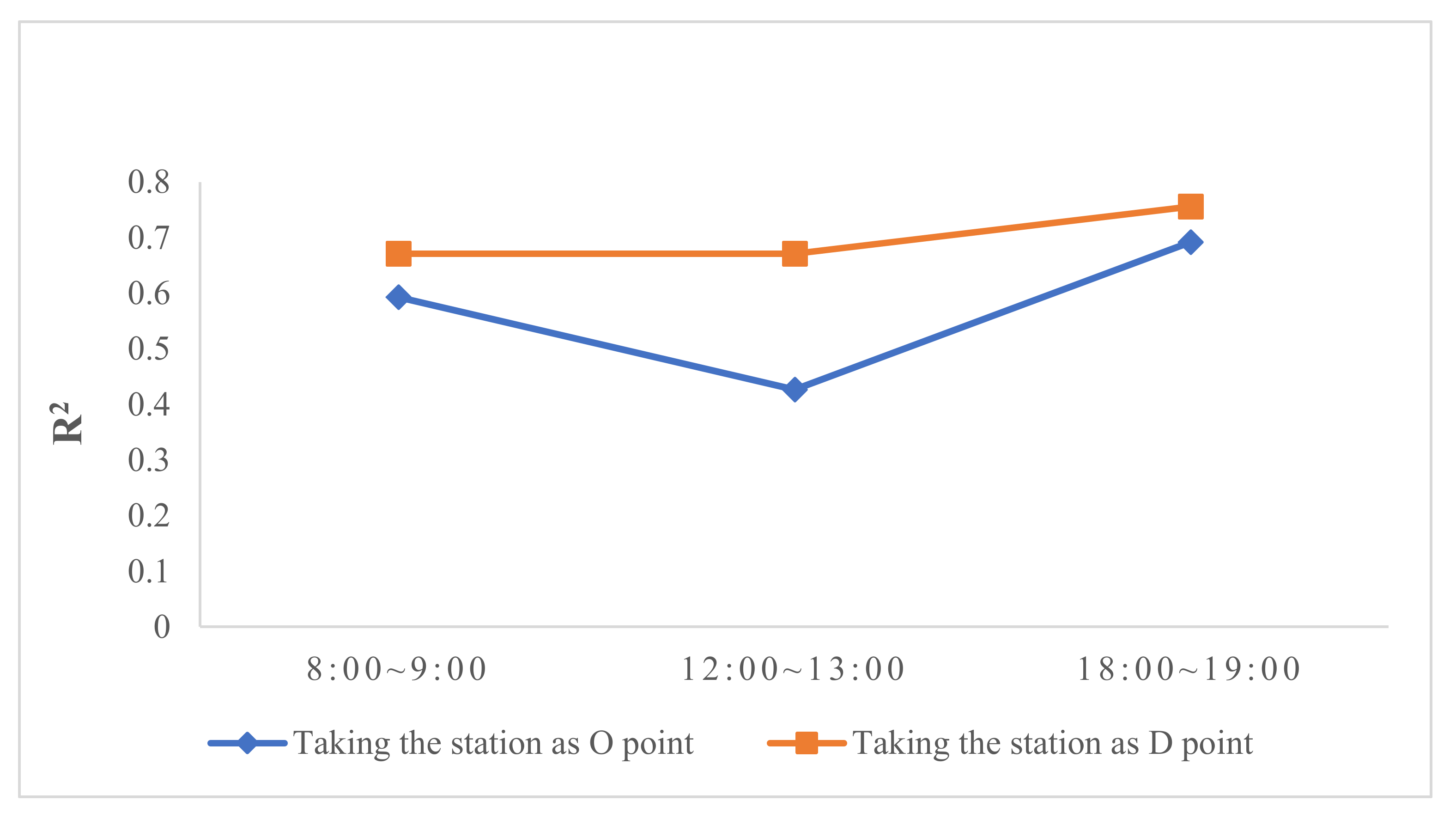
4.2. Model Evaluation

To illustrate the effectiveness of the method proposed in this paper for analyzing the spatiotemporal characteristics of bike-sharing usage, the goodness of fit ($R^2$) and condition number were selected as the effectiveness evaluation indexes. The relationship between the bike-sharing usage records as origin (O) and destination (D) points and independent variables were analyzed by GWR during the morning peak, off peak, and evening peak. Goodness of fit is shown in Figure 5. It can be seen that the degree of fit for the GWR model is relatively high. In addition, the maximum of the condition number for the GWR model in different periods is listed in

Table 6. The maximum of the condition number in different periods.

Period	The Maximum of the Condition Number
	Station as O Point	Station as D Point
8:00~9:00	16.3	26.0
12:00~13:00	23.2	25.0
18:00~19:00	25.6	25.3

, showing that each independent variable was less than 30. As can be seen, the GWR regression results were stable and reliable.

4.3. The Effect of Independent Variables on Bike-Sharing Usage

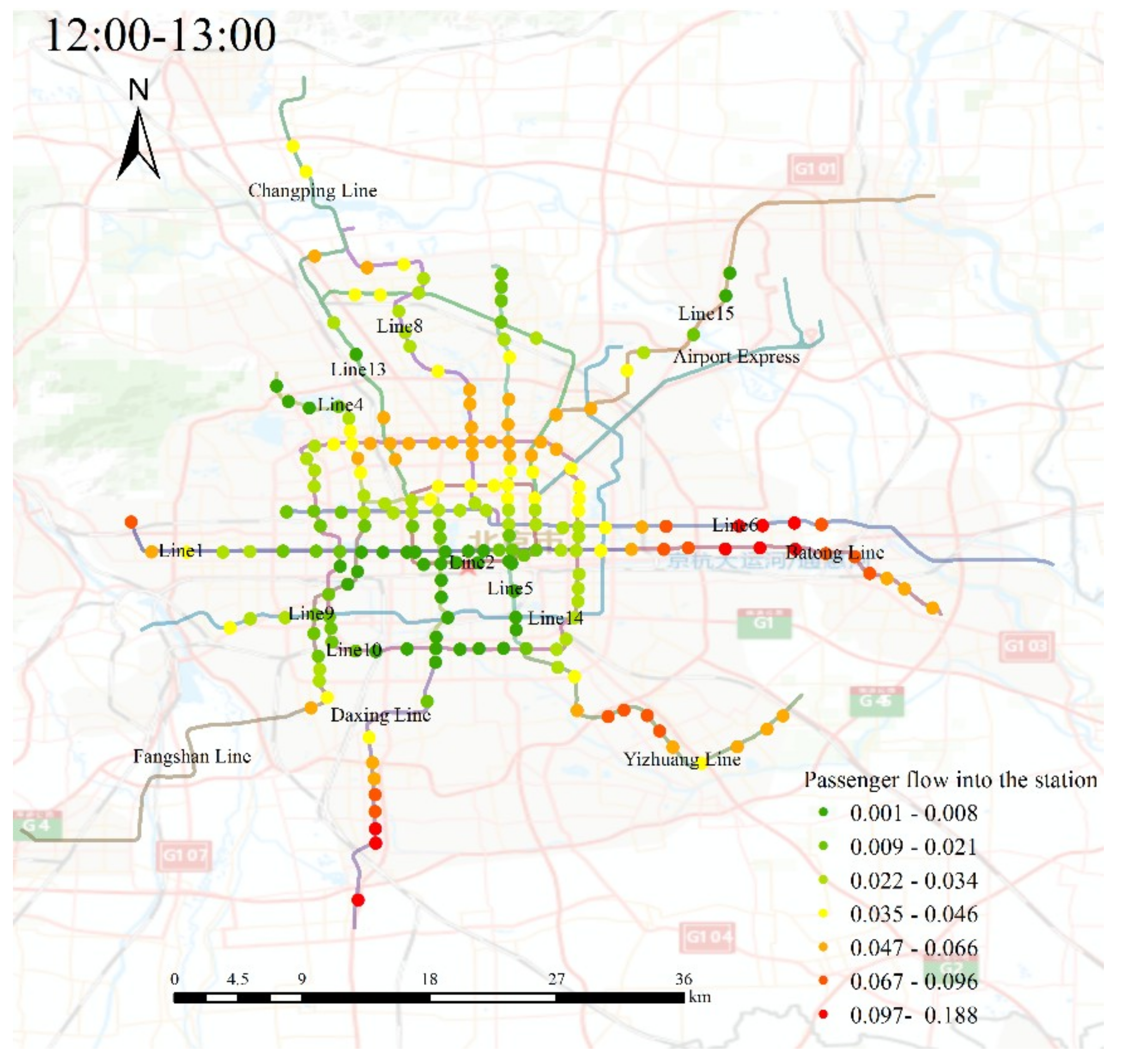
4.3.1. The Effect of Passenger Flow on Bike-Sharing Usage

The effect of the passenger flow on the bike-sharing usage differs by period. Based on passenger flow characteristics, we analyzed the effect of the passenger flow on the bike-sharing usage during the morning peak, off peak, and evening peak. Taking stations as D points, the relationship between the passenger flow into the station and the bike-sharing usage during the morning peak is shown in Figure 6. Passengers’ use of bike-sharing to connect to the subway during the morning peak exhibited strong local characteristics. Bike-sharing usage around the stations within the north fourth ring road of Beijing was greatly affected by passenger flow. Accordingly, the relevant management departments should focus on the connection between other regions and the north fourth ring road of Beijing when dispatching bikes.

Taking stations as D points, the relationship between the passenger flow into the station and the bike-sharing usage during the off peak is shown in Figure 7. During the off peak, bike-sharing usage that was greatly affected by passenger flow into the station was mainly distributed beyond the fourth ring road—perhaps because commuters working in the city center within the fourth ring road, who are the main service group of the subway, do not choose to go home at noon.

The bike-sharing usage during the evening peak was greatly affected by the passenger flow out of the station. Taking stations as O points, the relationship between the passenger flow out of the station and the bike-sharing usage during the evening peak is shown in Figure 8. Areas affected by the passenger flow out of the stations were mainly distributed in suburban stations located on Line 1 and the north fourth ring road of Beijing, China. In these areas, passengers preferred to use bike-sharing to travel between the station and home.

4.3.2. The Effect of Land Use on Bike-Sharing Usage

Our analysis revealed that the effect of land use on the bike-sharing usage showed opposite characteristics for O versus D points. Taking D points as an example, we analyzed the effect of the land use on the bike-sharing usage. During the morning peak, the bike-sharing usage was mainly related to the working land area around rail transit stations. This relationship is shown in Figure 9. Primarily, the bike-sharing usage at two types of stations was greatly affected by working land area. The first were stations in the north of Beijing, which were near much residential land. Many passengers entering these stations who preferred to use bike-sharing as an important mode of travel. The second were stations representing Zhongguancun on the north fourth ring road, which were near large amounts of working land. Some workers also used bike-sharing as an attendance tool. During the evening peak, bike-sharing usage was mainly related to the residential land around rail transit stations. This relationship is shown in Figure 10. A clear difference between north and south was noted in the bike-sharing usage on residential land area during the evening peak. Compared with those living in the northern region, residents around the stations in the southern region were more willing to use bike-sharing to return home from work.

4.3.3. The Effect of Bus Lines on Bike-Sharing Usage

The effect of bus lines on the bike-sharing usage was mainly reflected in connecting bus lines and collinear bus lines; we selected the evening peak for analysis. Figure 11 shows the relationship between connecting bus lines and the bike-sharing usage and Figure 12 is the relationship between collinear bus lines and the bike-sharing usage during the evening peak.

In the Chaoyang district, connecting bus lines and collinear bus lines often correlated positively with the bike-sharing usage. Most passengers return from their work offices (in the urban center) to their suburban residence during the evening peak. Due to having access to the developed bus network around the rail transit stations in the Chaoyang district, some users of bike-sharing choose to get on buses instead of subways.

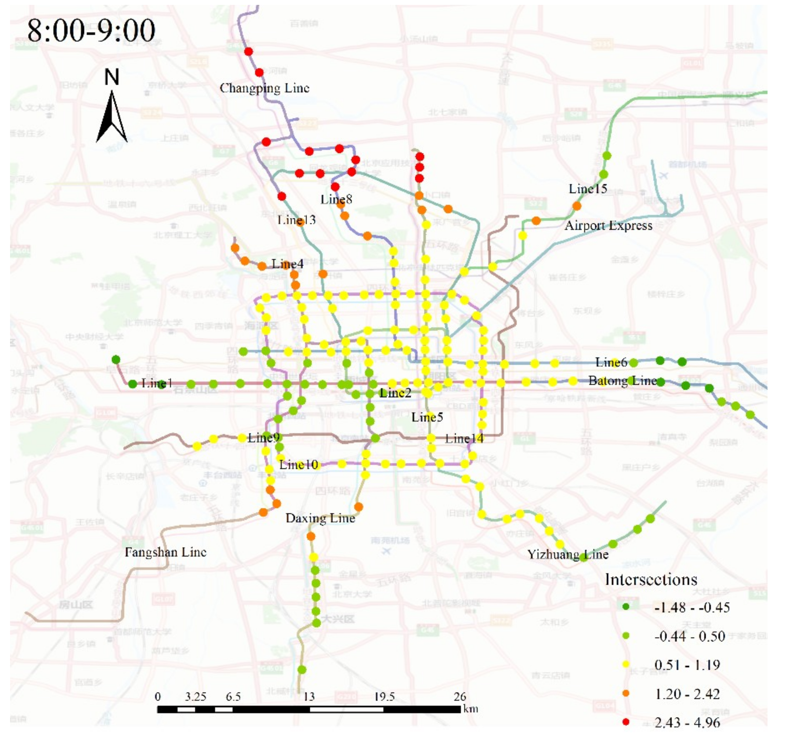
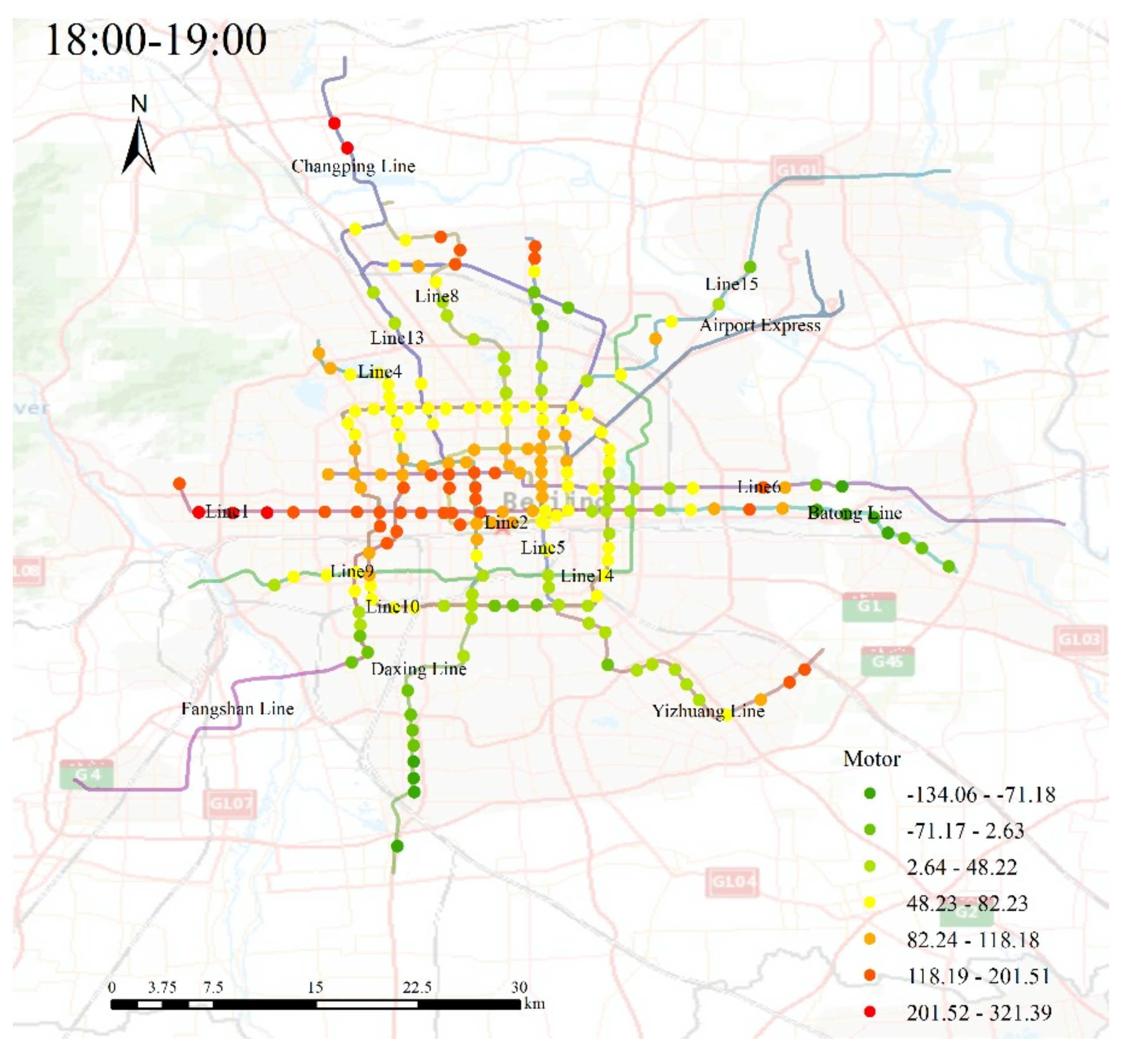
4.3.4. The Effect of Road-Network Characteristics on Bike-Sharing Usage

Road-network characteristics were also one of the most important influences on bike-sharing. The morning peak and evening peak were selected for analysis using the number of intersections and motor-vehicle lane density, respectively. Figure 13 shows the relationship between the number of intersections around rail transit stations and the bike-sharing usage during the morning peak. Figure 14 depicts the relationship between the motor-vehicle lane density and the bike-sharing usage during the evening peak, showing that travelers in the northern suburbs of Beijing, China were more concerned about the number of road intersections near their destinations. However, travelers in the central and western regions of Beijing, China were more sensitive to motor-vehicle lane density.

5. Conclusions

Bike-sharing greatly increases the convenience of travel for residents, especially when connecting stations and other places. Based on historical bike-sharing usage records, we used a GWR model to analyze the spatiotemporal characteristics of bike-sharing for the entire rail transit network of Beijing, China. This study can be summarized as follows:

• The bike-sharing usage around rail transit stations is mainly affected by the passenger flow into and out of stations, land use, bus lines, and road-network characteristics. We built a GWR model to capture the spatiotemporal characteristics of the bike-sharing usage around rail transit stations considering the passenger flow and built environment variables;
• From the time perspective, the characteristics of the bike-sharing usage around rail transit stations during the morning and evening peak hours show clear differences. The bike-sharing usage during the morning peak is affected by the passenger flow into the station, working land area, collinear bus lines, and number of road intersections. The bike-sharing usage during evening peak is affected by the passenger flow out of the station, residential land area, connecting bus line, and motor-vehicle lane density;
• From the spatial perspective, the bike-sharing usage around rail transit stations has obvious partition characteristics. The bike-sharing usage around rail transit stations near the north fourth ring road of Beijing, is heavily affected by the passenger flow. In the north and south of Beijing, bike-sharing usage is mainly affected by working land area and residential land area. In the Chaoyang district, the bike-sharing usage is more sensitive to connecting bus lines and collinear bus lines. The effect of the number of road intersections is mainly reflected in the northern suburbs, and the effect of the motor-vehicle lane density is mainly reflected in the central and western regions of Beijing.

This work can provide technical support for the operations and management of bike-sharing services while serving as a reference for future studies on the connection between bike-sharing and other transportation modes and the influence of TOD development on bike-sharing. This method can be applied to the analysis of bike-sharing usage in other cities with the appropriate adjustments.

In our work, we only analyzed the spatiotemporal characteristics of bike-sharing usage around rail transit stations in Beijing, China, which was limited by our obtained data. The current work could be extended by obtaining more data from other cities. The spatiotemporal characteristics of bike-sharing usage in multiple cities could be compared, and more findings would be given.

References

1. Du, M.; Cheng, L. Better understanding the characteristics and influential factors of different travel patterns in free-floating bike sharing: Evidence from Nanjing, China. Sustainability 2018, 10, 1244. [Google Scholar] [CrossRef] [Green Version]
2. Zhang, Y.; Mi, Z. Environmental benefits of bike sharing: A big data-based analysis. Appl. Energy 2018, 220, 296–301. [Google Scholar] [CrossRef]
3. Li, Y.; Zhu, Z.; Guo, X. Operating Characteristics of Dockless Bike-Sharing Systems near Metro Stations: Case Study in Nanjing City, China. Sustainability 2019, 11, 2256. [Google Scholar] [CrossRef] [Green Version]
4. Caggiani, L.; Camporeale, R.; Marinelli, M.; Ottomanelli, M. User satisfaction based model for resource allocation in bike-sharing systems. Transp. Policy 2019, 80, 117–126. [Google Scholar] [CrossRef]
5. Cerutti, P.S.; Martins, R.D.; Macke, J.; Sarate, J.A.R. “Green, but not as green as that”: An analysis of a Brazilian bike-sharing system. J. Clean. Prod. 2019, 217, 185–193. [Google Scholar] [CrossRef]
6. Ma, X.; Ji, Y.; Yang, M.; Jin, Y.; Tan, X. Understanding bikeshare mode as a feeder to metro by isolating metro-bikeshare transfers from smart card data. Transp. Policy 2018, 71, 57–69. [Google Scholar] [CrossRef]
7. Rixey, R.A. Station-level forecasting of bikesharing ridership: Station network effects in three US systems. Transp. Res. Rec. 2013, 2387, 46–55. [Google Scholar] [CrossRef] [Green Version]
8. Zhou, Y.; Wang, L.; Zhong, R.; Tan, Y. A Markov Chain Based Demand Prediction Model for Stations in Bike Sharing Systems. Math. Probl. Eng. 2018, 2018, 8028714. [Google Scholar] [CrossRef] [Green Version]
9. Xu, C.; Ji, J.; Liu, P. The station-free sharing bike demand forecasting with a deep learning approach and large-scale datasets. Transp. Res. Part C Emerg. Technol. 2018, 95, 47–60. [Google Scholar] [CrossRef]
10. El-Assi, W.; Mahmoud, M.S.; Habib, K.N. Effects of built environment and weather on bike sharing demand: A station level analysis of commercial bike sharing in Toronto. Transportation 2017, 44, 589–613. [Google Scholar] [CrossRef]
11. Zhang, J.; Meng, M.; David, Z. A dynamic pricing scheme with negative prices in dockless bike sharing systems. Transp. Res. Part B Methodol. 2019, 127, 201–224. [Google Scholar] [CrossRef]
12. Ruch, C.; Warrington, J.; Morari, M. Rule-based price control for bike sharing systems. In Proceedings of the 2014 European Control Conference (ECC), Strasbourg, France, 24–27 June 2014; pp. 708–713. [Google Scholar]
13. Haider, Z.; Nikolaev, A.; Kang, J.E.; Kwon, C. Inventory rebalancing through pricing in public bike sharing systems. Eur. J. Oper. Res. 2018, 270, 103–117. [Google Scholar] [CrossRef]
14. Caggiani, L.; Camporeale, R.; Ottomanelli, M.; Szeto, W.Y. A modeling framework for the dynamic management of free-floating bike-sharing systems. Transp. Res. Part C Emerg. Technol. 2018, 87, 159–182. [Google Scholar] [CrossRef]
15. Gu, T.; Kim, I.; Currie, G. Measuring immediate impacts of a new mass transit system on an existing bike-share system in China. Transp. Res. Part A Policy Pract. 2019, 124, 20–39. [Google Scholar] [CrossRef]
16. Zhou, X. Understanding spatiotemporal patterns of biking behavior by analyzing massive bike sharing data in Chicago. PLoS ONE 2015, 10, e0137922. [Google Scholar] [CrossRef]
17. Li, W.; Sun, W.; Li, G.; Jin, B.; Wu, W.; Cui, P.; Zhao, G. Transmission mechanism between energy prices and carbon emissions using geographically weighted regression. Energy Policy 2018, 115, 434–442. [Google Scholar] [CrossRef]
18. Peng, C.; OuYang, Z.; Liu, Y. Understanding bike sharing use over time by employing extended technology continuance theory. Transp. Res. Part A Policy Pract. 2019, 124, 433–443. [Google Scholar]
19. Li, Y.; Szeto, W.; Long, J.; Shui, C. A multiple type bike repositioning problem. Transp. Res. Part B Methodol. 2016, 90, 263–278. [Google Scholar] [CrossRef] [Green Version]
20. Chemla, D.; Meunier, F.; Calvo, R.W. Bike sharing systems: Solving the static rebalancing problem. Discret. Optim. 2013, 10, 120–146. [Google Scholar] [CrossRef]
21. Shui, C.; Szeto, W. An artificial bee colony algorithm for public bike repositioning problem. In Proceedings of the ATRF 2015 Australasian Transport Research Forum, Sydney, Australia, 30 September–2 October 2015; The National Academies of Sciences, Engineering, and Medicine: Washington, DC, USA, 2015. [Google Scholar]
22. Paul, F.; Bogenberger, K. Evaluation-method for a station based urban-pedelec sharing system. Transp. Res. Procedia 2014, 4, 482–493. [Google Scholar] [CrossRef] [Green Version]
23. Manca, F.; Sivakumar, A.; Polak, J.W. The effect of social influence and social interactions on the adoption of a new technology: The use of bike sharing in a student population. Transp. Res. Part C Emerg. Technol. 2019, 105, 611–625. [Google Scholar] [CrossRef]
24. Tran, T.D.; Ovtracht, N.; D’arcier, B.F. Modeling bike sharing system using built environment factors. Procedia Cirp 2015, 30, 293–298. [Google Scholar] [CrossRef]
25. Mateo-Babiano, I.; Bean, R.; Corcoran, J.; Pojani, D. How does our natural and built environment affect the use of bicycle sharing? Transp. Res. Part A Policy Pract. 2016, 94, 295–307. [Google Scholar] [CrossRef] [Green Version]
26. Abolhassani, L.; Afghari, A.P.; Borzadaran, H.M. Public preferences towards bicycle sharing system in developing countries: The case of Mashhad, Iran. Sustain. Cities Soc. 2019, 44, 763–773. [Google Scholar] [CrossRef]
27. Duarte, F.; Rojas, F. Intermodal connectivity to BRT: A comparative analysis of Bogotá and Curitiba. J. Public Transp. 2012, 15, 1. [Google Scholar] [CrossRef] [Green Version]
28. Wang, X.; Lindsey, G.; Schoner, J.E.; Harrison, A. Modeling bike share station activity: Effects of nearby businesses and jobs on trips to and from stations. J. Urban Plan. Dev. 2015, 142, 04015001. [Google Scholar] [CrossRef] [Green Version]
29. Zhang, Y.; Thomas, T.; Brussel, M.; Van Maarseveen, M. Exploring the impact of built environment factors on the use of public bikes at bike stations: Case study in Zhongshan, China. J. Transp. Geogr. 2017, 58, 59–70. [Google Scholar] [CrossRef]
30. Wang, Z.-j.; Chen, F.; Xu, T.-k. Interchange between metro and other modes: Access distance and catchment area. J. Urban Plan. Dev. 2016, 142, 04016012. [Google Scholar] [CrossRef]
31. Ji, Y.; Ma, X.; Yang, M.; Jin, Y.; Gao, L. Exploring spatially varying influences on metro-bikeshare transfer: A geographically weighted poisson regression approach. Sustainability 2018, 10, 1526. [Google Scholar] [CrossRef] [Green Version]
32. Rogerson, P.A. Statistical Methods for Geography: A Student’s Guide; Sage Publications Limited: London, UK, 2019. [Google Scholar]
33. Lee, J.; Li, S. Extending Moran’s index for measuring spatiotemporal clustering of geographic events. Geogr. Anal. 2017, 49, 36–57. [Google Scholar] [CrossRef]
34. Shen, C.; Li, C.; Si, Y. Spatio-temporal autocorrelation measures for nonstationary series: A new temporally detrended spatio-temporal Moran’s index. Phys. Lett. A 2016, 380, 106–116. [Google Scholar] [CrossRef]
35. Chao, L.; Zhang, K.; Li, Z.; Zhu, Y.; Wang, J.; Yu, Z. Geographically weighted regression based methods for merging satellite and gauge precipitation. J. Hydrol. 2018, 558, 275–289. [Google Scholar] [CrossRef]
36. Fotheringham, A.S.; Charlton, M.E.; Brunsdon, C. Geographically weighted regression: A natural evolution of the expansion method for spatial data analysis. Environ. Plan. A 1998, 30, 1905–1927. [Google Scholar] [CrossRef]
37. Zhou, Q.; Wang, C.; Fang, S. Application of geographically weighted regression (GWR) in the analysis of the cause of haze pollution in China. Atmos. Pollut. Res. 2019, 10, 835–846. [Google Scholar] [CrossRef]
38. Dziauddin, M.F. Estimating land value uplift around light rail transit stations in Greater Kuala Lumpur: An empirical study based on geographically weighted regression (GWR). Res. Transp. Econ. 2019, 74, 10–20. [Google Scholar] [CrossRef]
39. Nguyen, Q.-H. Understanding Factors Affecting the Outbreak of Malaria Using Locally-Compensated Ridge Geographically Weighted Regression: Case Study in DakNong, Vietnam. In Advances and Applications in Geospatial Technology and Earth Resources: Proceedings of the International Conference on Geo-Spatial Technologies and Earth Resources 2017; Springer: Berlin/Heidelberg, Germany, 2017; p. 166. [Google Scholar]
Figure 1. Rail transit stations in Beijing, China.
Sustainability 12 01299 g001
Figure 2. Bike-sharing usage records during different periods on 19 April 2018.
Sustainability 12 01299 g002
Figure 3. Statistical data for passenger flow into stations.
Sustainability 12 01299 g003
Figure 4. Statistical data for passenger flow out of stations.
Sustainability 12 01299 g004
Figure 5. Goodness of fit in different periods.
Sustainability 12 01299 g005
Figure 6. Relationship between passenger flow into the station and bike-sharing usage during the morning peak.
Sustainability 12 01299 g006
Figure 7. Relationship between passenger flow into the station and bike-sharing usage during the off peak.
Sustainability 12 01299 g007
Figure 8. Relationship between passenger flow out of the station and bike-sharing usage during the evening peak.
Sustainability 12 01299 g008
Figure 9. Relationship between working land area and bike-sharing usage during the morning peak.
Sustainability 12 01299 g009
Figure 10. Relationship between residential land area and bike-sharing usage during the evening peak.
Sustainability 12 01299 g010
Figure 11. Relationship between connecting bus lines and bike-sharing usage during the evening peak.
Sustainability 12 01299 g011
Figure 12. Relationship between collinear bus lines and bike-sharing usage during the evening peak.
Sustainability 12 01299 g012
Figure 13. Relationship between number of intersections and bike-sharing usage during the morning peak.
Sustainability 12 01299 g013
Figure 14. Relationship between motor-vehicle lane density and bike-sharing usage during the evening peak.
Sustainability 12 01299 g014