Showcasing Relationships between Neighborhood Design and Wellbeing Toronto Indicators

 ,
, 
Abstract
1. Introduction
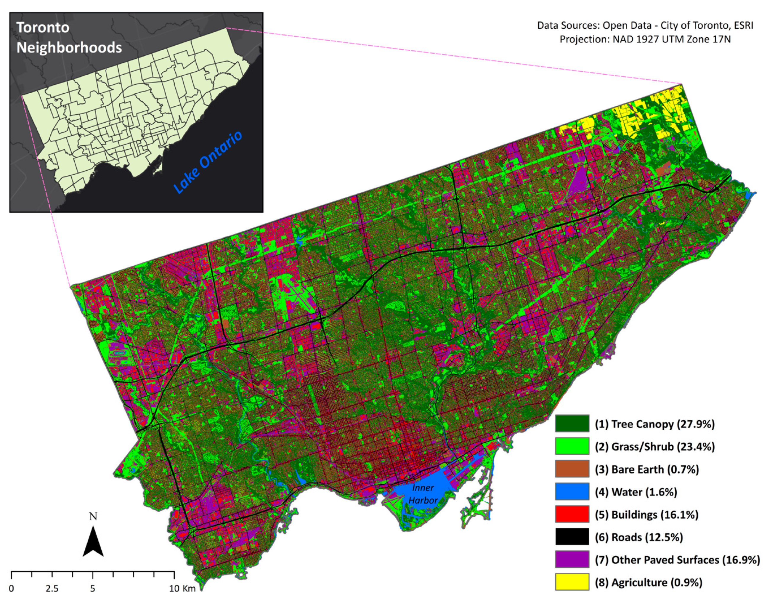
2. Study Area
3. Materials and Methods
3.1. Wellbeing Toronto Indicators
3.2. Streetscape Configuration and Diversity
3.3. Data Analysis
4. Results
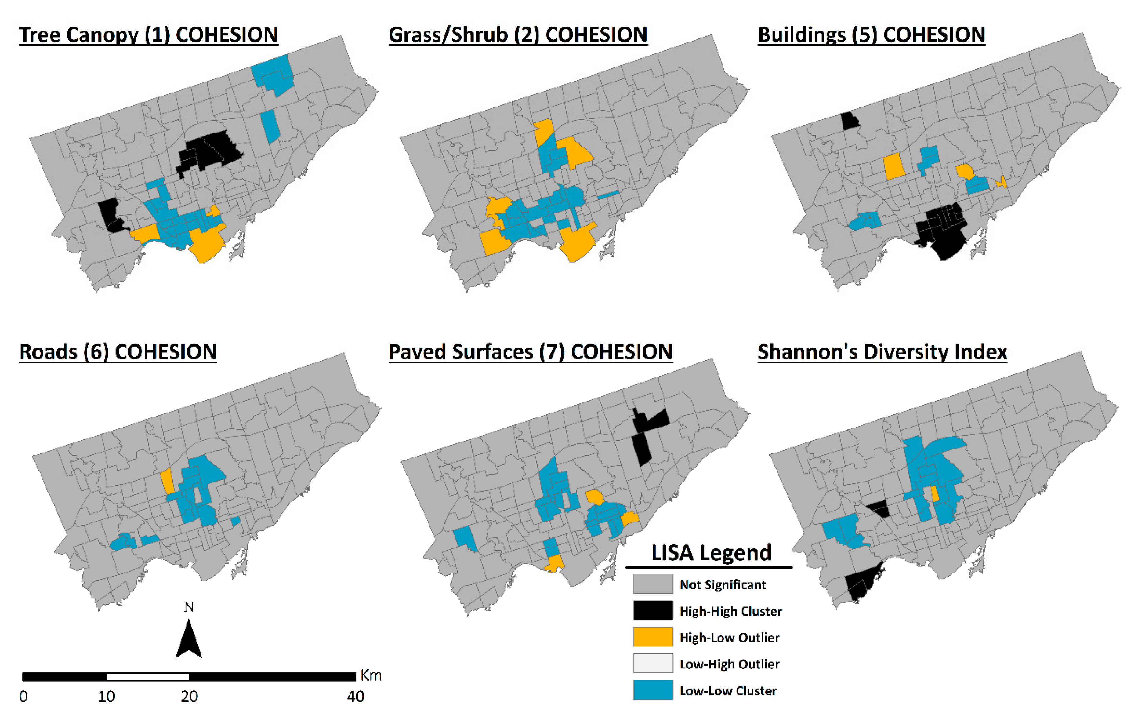
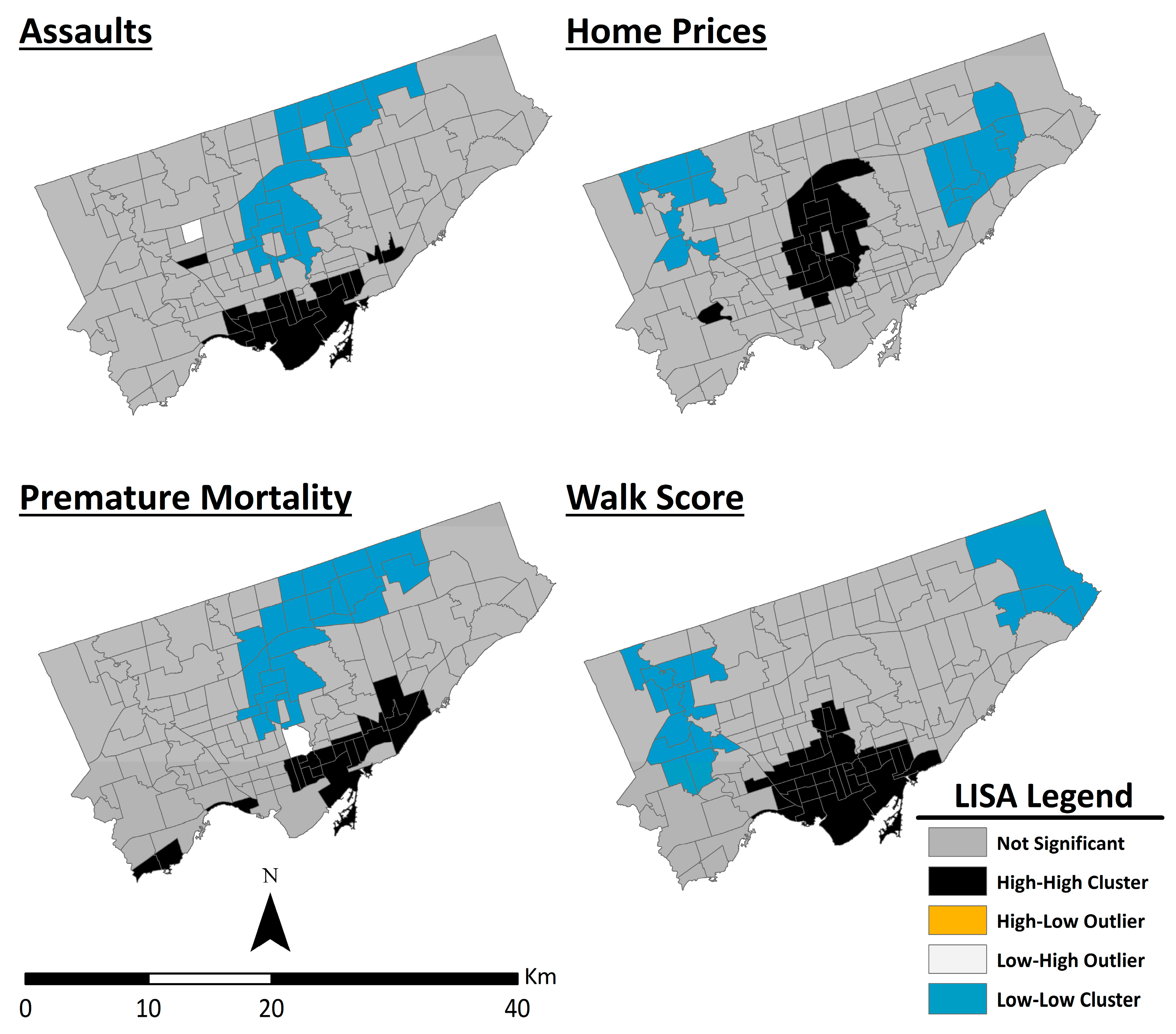
4.1. Exploratory Spatial Pattern Analysis
4.2. Global Correlation Coefficients
4.3. Spatial Autoregressions
5. Discussion
5.1. Importance of Relationships
5.2. Sustainable Urbanization: Building Resilience
6. Conclusions
Supplementary Materials
Author Contributions
Funding
Acknowledgments
Conflicts of Interest
Appendix A
Appendix A.1
Appendix A.2
Appendix A.3
References
- UN, U.N. World Population Prospects: 2017 Revision; United Nations: Department of Economic and Social Affairs: New York, NY, USA, 2017; pp. 1–53. [Google Scholar]
- Crane, P.; Kinzig, A. Nature in the Metropolis. Science 2005, 308, 1225. [Google Scholar] [CrossRef] [PubMed]
- UN, U.N. World Urbanization Prospects: The 2018 Revision; Economic and Social Affairs: New York, NY, USA, 2018; pp. 1–2. [Google Scholar]
- Batty, M. When all the word’s a city. Environ. Plan. A 2011, 43, 765–772. [Google Scholar] [CrossRef]
- Wu, J. Urban sustainability: An inevitable goal of landscape research. Landsc. Ecol. 2010, 25, 1–4. [Google Scholar] [CrossRef]
- Wu, J. Urban ecology and sustainability: The state-of-the-science and future directions. Landsc. Urban Plan. 2014, 125, 209–221. [Google Scholar] [CrossRef]
- Wu, J. (Jingle) Making the Case for Landscape Ecology An Effective Approach to Urban Sustainability. Landsc. Jrnl. 2008, 27, 41–50. [Google Scholar] [CrossRef]
- Shaker, R.R. The well-being of nations: An empirical assessment of sustainable urbanization for Europe. Int. J. Sustain. Dev. World Ecol. 2015, 22, 375–387. [Google Scholar] [CrossRef]
- Alberti, M. Advances in Urban Ecology: Integrating Humans And Ecological Processes in Urban Ecosystems; Springer: New York, NY, USA, 2008; ISBN 978-0-387-75509-0. [Google Scholar]
- Carpenter, S.R.; Mooney, H.A.; Agard, J.; Capistrano, D.; DeFries, R.S.; Díaz, S.; Dietz, T.; Duraiappah, A.K.; Oteng-Yeboah, A.; Pereira, H.M.; et al. Science for managing ecosystem services: Beyond the Millennium Ecosystem Assessment. PNAS 2009, 106, 1305–1312. [Google Scholar] [CrossRef]
- Forman, R.T.T.; Wu, J. Where to put the next billion people. Nat. News 2016, 537, 608. [Google Scholar] [CrossRef]
- Grimm, N.B.; Faeth, S.H.; Golubiewski, N.E.; Redman, C.L.; Wu, J.; Bai, X.; Briggs, J.M. Global Change and the Ecology of Cities. Science 2008, 319, 756–760. [Google Scholar] [CrossRef]
- Seto, K.C.; Güneralp, B.; Hutyra, L.R. Global forecasts of urban expansion to 2030 and direct impacts on biodiversity and carbon pools. PNAS 2012, 109, 16083–16088. [Google Scholar] [CrossRef]
- Shaker, R.R.; Altman, Y.; Deng, C.; Vaz, E.; Forsythe, K.W. Investigating urban heat island through spatial analysis of New York City streetscapes. J. Clean. Prod. 2019, 233, 972–992. [Google Scholar] [CrossRef]
- Steffen, W.; Richardson, K.; Rockström, J.; Cornell, S.E.; Fetzer, I.; Bennett, E.M.; Biggs, R.; Carpenter, S.R.; de Vries, W.; de Wit, C.A.; et al. Planetary boundaries: Guiding human development on a changing planet. Science 2015, 347, 1259855. [Google Scholar] [CrossRef] [PubMed]
- Turner, M.G.; Gardner, R.H. Landscape Ecology in Theory And Practice: Pattern And Process, 2nd ed.; Springer: New York, NY, USA, 2015; ISBN 978-1-4939-2793-7. [Google Scholar]
- Ceballos, G.; Ehrlich, P.R.; Dirzo, R. Biological annihilation via the ongoing sixth mass extinction signaled by vertebrate population losses and declines. PNAS 2017, 114, E6089–E6096. [Google Scholar] [CrossRef] [PubMed]
- Foley, J.A.; DeFries, R.; Asner, G.P.; Barford, C.; Bonan, G.; Carpenter, S.R.; Chapin, F.S.; Coe, M.T.; Daily, G.C.; Gibbs, H.K.; et al. Global Consequences of Land Use. Science 2005, 309, 570–574. [Google Scholar] [CrossRef]
- Hansen, M.C.; Potapov, P.V.; Moore, R.; Hancher, M.; Turubanova, S.A.; Tyukavina, A.; Thau, D.; Stehman, S.V.; Goetz, S.J.; Loveland, T.R.; et al. High-Resolution Global Maps of 21st-Century Forest Cover Change. Science 2013, 342, 850–853. [Google Scholar] [CrossRef]
- Hoegh-Guldberg, O.; Bruno, J.F. The Impact of Climate Change on the World’s Marine Ecosystems. Science 2010, 328, 1523–1528. [Google Scholar] [CrossRef]
- Liu, J.; Dietz, T.; Carpenter, S.R.; Alberti, M.; Folke, C.; Moran, E.; Pell, A.N.; Deadman, P.; Kratz, T.; Lubchenco, J.; et al. Complexity of Coupled Human and Natural Systems. Science 2007, 317, 1513–1516. [Google Scholar] [CrossRef]
- Pickett, S.T.A.; Cadenasso, M.L.; Grove, J.M.; Boone, C.G.; Groffman, P.M.; Irwin, E.; Kaushal, S.S.; Marshall, V.; McGrath, B.P.; Nilon, C.H.; et al. Urban ecological systems: Scientific foundations and a decade of progress. J. Environ. Manag. 2011, 92, 331–362. [Google Scholar] [CrossRef]
- Shaker, R.R.; Yakubov, A.D.; Nick, S.M.; Vennie-Vollrath, E.; Ehlinger, T.J.; Forsythe, K.W. Predicting aquatic invasion in Adirondack lakes: A spatial analysis of lake and landscape characteristics. Ecosphere 2017, 8, e01723. [Google Scholar] [CrossRef]
- Rockström, J.; Steffen, W.; Noone, K.; Persson, Å.; Chapin, F.S.I.; Lambin, E.; Lenton, T.; Scheffer, M.; Folke, C.; Schellnhuber, H.J.; et al. Planetary Boundaries: Exploring the Safe Operating Space for Humanity. Ecol. Soc. 2009, 14, 32. [Google Scholar] [CrossRef]
- Rockström, J.; Steffen, W.; Noone, K.; Persson, Å.; Chapin, F.S.; Lambin, E.F.; Lenton, T.M.; Scheffer, M.; Folke, C.; Schellnhuber, H.J.; et al. A safe operating space for humanity. Nature 2009, 461, 472–475. [Google Scholar] [CrossRef] [PubMed]
- Batty, M. The Size, Scale, and Shape of Cities. Science 2008, 319, 769. [Google Scholar] [CrossRef] [PubMed]
- Grosskurth, J. Ambition and reality in modeling: A case study on public planning for regional sustainability. Sustain. Sci. Pract. Policy 2007, 3, 3–11. [Google Scholar] [CrossRef]
- Campbell, H. Sustainable Development: Can the Vision be Realized? Plan. Theory Pract. 2000, 1, 259–284. [Google Scholar] [CrossRef]
- Shaker, R.R.; Zubalsky, S.L. Examining patterns of sustainability across Europe: A multivariate and spatial assessment of 25 composite indices. Int. J. Sustain. Dev. World Ecol. 2015, 22, 1–13. [Google Scholar] [CrossRef]
- Chifos, C. The Sustainable Communities Experiment in the United States: Insights from Three Federal-Level Initiatives. J. Plan. Educ. Res. 2016, 26, 435–449. [Google Scholar] [CrossRef]
- Godschalk, D.R. Land Use Planning Challenges: Coping with Conflicts in Visions of Sustainable Development and Livable Communities. J. Am. Plan. Assoc. 2004, 70, 5–13. [Google Scholar] [CrossRef]
- Edward, J.; Jepson, J. Human Nature and Sustainable Development: A Strategic Challenge for Planners. J. Plan. Lit. 2004, 19, 3–15. [Google Scholar]
- Hezri, A.A.; Dovers, S.R. Sustainability indicators, policy and governance: Issues for ecological economics. Ecol. Econ. 2006, 60, 86–99. [Google Scholar] [CrossRef]
- Keiner, M. (Ed.) The Future of Sustainability; Springer: Amsterdam, The Netherlands, 2006; ISBN 978-1-4020-4734-3. [Google Scholar]
- Tischendorf, L.; Fahrig, L. On the usage and measurement of landscape connectivity. Oikos 2000, 90, 7–19. [Google Scholar] [CrossRef]
- Opdam, P.; Luque, S.; Nassauer, J.; Verburg, P.H.; Wu, J. How can landscape ecology contribute to sustainability science? Landsc. Ecol. 2018, 33, 1–7. [Google Scholar] [CrossRef]
- Naveh, Z. Landscape ecology and sustainability. Landsc. Ecol. 2007, 22, 1437–1440. [Google Scholar] [CrossRef]
- Botequilha Leitão, A.; Ahern, J. Applying landscape ecological concepts and metrics in sustainable landscape planning. Landsc. Urban Plan. 2002, 59, 65–93. [Google Scholar] [CrossRef]
- Mander, Ü.; Uuemaa, E. Landscape assessment for sustainable planning. Ecol. Ind. 2010, 10, 1–3. [Google Scholar] [CrossRef]
- Spellberg, I.F. Evaluation and Assessment For Conservation: Ecological Guidelines for Determining Priorities for Nature Conservation; Springer: Amsterdam, The Netherlands, 1994; ISBN 978-0-412-44280-3. [Google Scholar]
- Shaker, R.R. Examining sustainable landscape function across the Republic of Moldova. Habitat Intern. 2018, 72, 77–91. [Google Scholar] [CrossRef]
- Tobler, W.R. A Computer Movie Simulating Urban Growth in the Detroit Region. Econ. Geogr. 1970, 46, 234–240. [Google Scholar] [CrossRef]
- Meerow, S.; Newell, J.P. Spatial planning for multifunctional green infrastructure: Growing resilience in Detroit. Landsc. Urban Plan. 2017, 159, 62–75. [Google Scholar] [CrossRef]
- Allen, R.; Campsie, P. Implementing The Growth Plan For The Greater Golden Horseshoe: Has The Strategic Regional Vision Been Compromised? Neptis Foundation: Toronto, ON, Canada, 2015; ISBN 978-0-9739888-6-4. [Google Scholar]
- Relph, E. Toronto: Transformations in a City and Its Region; University of Pennsylvania Press: Philadelphia, PA, USA, 2014; ISBN 978-0-8122-4542-4. [Google Scholar]
- Hulchanski, J.D. The Three Cities Within Toronto: Income Polarization among Toronto’s Neighbourhoods, 1970-2005; University of Toronto: Toronto, ON, Canada, 2011; ISBN 978-0-7727-1478-7. [Google Scholar]
- Conway, T.; Hackworth, J. Urban pattern and land cover variation in the greater Toronto area. Can. Geogr. Géogr. Can. 2007, 51, 43–57. [Google Scholar] [CrossRef]
- Sahely, H.R.; Dudding, S.; Kennedy, C.A. Estimating the urban metabolism of Canadian cities: Greater Toronto Area case study. Can. J. Civ. Eng. 2003, 30, 468–483. [Google Scholar] [CrossRef]
- Zukin, S.; Kasinitz, P.; Chen, X. Global Cities, Local Streets: Everyday Diversity from New York to Shanghai; Routledge: New York, NY, USA, 2015; ISBN 978-1-317-68974-4. [Google Scholar]
- Murdie, R.; Bourne, L.; Hulchanski, J.D.; Maaranen, R.; Walks, R.A. Diversity and Concentration in Canadian Immigration: Trends in Tronto, Montreal and Vancouver, 1971-2006; University of Toronto: Cities Centre: Toronto, ON, Canada, 2008; pp. 1–12. [Google Scholar]
- TF, Toronto Foundation. Toronto’s Vital Signs; Toronto Foundation: Toronto, ON, Canada, 2018; pp. 1–90. [Google Scholar]
- Hayes, D. Historical Atlas of Toronto; Douglas & McIntyre: Vancouver, BC, Canada, 2009; ISBN 978-1-55365-497-1. [Google Scholar]
- Hiebert, D.; Schuurman, N.; Smith, H. Metropolis Project Multiculturalism “on the ground”: The social geography of immigrant and visible minority populations in Montreal, Toronto, and Vancouver, projected to 2017; Centre of Excellence for Research on Immigration and Diversity: Vancouver, BC, Canada, 2007; pp. 7–12. [Google Scholar]
- Fulford, R. Accidental City: The Transformation of Toronto; Houghton Mifflin Company: Boston, MA, USA, 1996; ISBN 978-0-395-77307-9. [Google Scholar]
- City of Toronto. TORONTO STRONG NEIGHBOURHOODS STRATEGY 2020; City of Toronto: Toronto, ON, Canada, 2014; pp. 1–42.
- Fraser Institute. Canada Must Grow Denser and More Populated: Op-ed. Available online: https://www.fraserinstitute.org/article/canada-must-grow-denser-and-more-populated (accessed on 17 December 2019).
- City of Toronto. Toronto at a Glance. Available online: https://www.toronto.ca/city-government/data-research-maps/toronto-at-a-glance/ (accessed on 17 December 2019).
- Filipowicz, J. Room to Grow: Comparing Urban Density in Canada and Abroad; Fraser Institute: Toronto, ON, Canada, 2018; pp. 1–14. [Google Scholar]
- Clayton, F.; Shi, H.Y. (Eva) WOW! Toronto Was the Second Fastest Growing Metropolitan Area and the Top Growing City in All of the United States and Canada. In WOW! Toronto Was the Second Fastest Growing Metropolitan Area and the Top Growing City in All of the United States and Canada; Ryerson University: Toronto, ON, Canada, 2019. [Google Scholar]
- Vaz, E.; Arsanjani, J.J. Predicting Urban Growth of the Greater Toronto Area - Coupling a Markov Cellular Automata with Document Meta-Analysis. J. Environ. Inf. 2016, 25, 71–80. [Google Scholar] [CrossRef]
- OPG. Ontario Provincial Government. Greenbelt Plan (2017); Government of Ontario: Ministry of Municipal Affairs and Housing: Toronto, ON, Canada, 2017; pp. 1–98.
- Brown, C.; Shaker, R.R.; Das, R. A review of approaches for monitoring and evaluation of urban climate resilience initiatives. Environ. Dev. Sustain. 2018, 20, 23–40. [Google Scholar] [CrossRef]
- Polèse, M.; Stren, R.E.; Stren, R. The Social Sustainability of Cities: Diversity and the Management of Change; University of Toronto Press: Toronto, ON, Canada, 2000; ISBN 978-0-8020-8320-3. [Google Scholar]
- Roots, B.; Chant, D.; Heidenreich, C. Special Places: The Changing Ecosystems of the Toronto Region; UBC Press: Vancouver, BC, Canada, 2011; ISBN 978-0-7748-4181-8. [Google Scholar]
- Bonnell, J.L. Reclaiming the Don: An Environmental History of Toronto’s Don River Valley; University of Toronto Press: Toronto, ON, Canada, 2014; ISBN 978-1-4426-9681-5. [Google Scholar]
- Racine, V. Human|Wildlife, Stitching The Fabric: Connectivity Strategies For Identified Gaps in Toronto’s Ravines; Ryerson University: Toronto, ON, Canada, 2017; pp. 1–96. [Google Scholar]
- City of Toronto. TORONTO MUNICIPAL CODE CHAPTER 658, RAVINE AND NATURAL FEATURE PROTECTION; City of Toronto: Toronto, ON, Canada, 2016; pp. 1–16. [Google Scholar]
- Michalos, A.C. Canadian Index of Well-Being; University of Waterloo: Waterloo, ON, Canada, 2006; pp. 1–66. [Google Scholar]
- CIW. How are Canadians Really Doing? The 2016 CIW National Report; University of Waterloo: Waterloo, ON, Canada, 2016; pp. 1–96. [Google Scholar]
- Huang, L.; Wu, J.; Yan, L. Defining and measuring urban sustainability: A review of indicators. Landsc. Ecol. 2015, 30, 1175–1193. [Google Scholar] [CrossRef]
- Shaker, R.R.; Sirodoev, I.G. Assessing sustainable development across Moldova using household and property composition indicators. Habitat Intern. 2016, 55, 192–204. [Google Scholar] [CrossRef]
- Shaker, R.R. A mega-index for the Americas and its underlying sustainable development correlations. Ecol. Indic. 2018, 89, 466–479. [Google Scholar] [CrossRef]
- Brugmann, J. Is there a method in our measurement? The use of indicators in local sustainable development planning. Local Environ. 1997, 2, 59–72. [Google Scholar] [CrossRef]
- Maclaren, V.W. Urban Sustainability Reporting. J. Am. Plan. Assoc. 1996, 62, 184–202. [Google Scholar] [CrossRef]
- Shen, L.-Y.; Jorge Ochoa, J.; Shah, M.N.; Zhang, X. The application of urban sustainability indicators—A comparison between various practices. Habitat Intern. 2011, 35, 17–29. [Google Scholar] [CrossRef]
- Hák, T.; Moldan, B.; Dahl, A.L. Sustainability Indicators: A Scientific Assessment; Island Press: Washington, DC, USA, 2012; ISBN 978-1-59726-628-4. [Google Scholar]
- Bell, S.; Morse, S. Sustainability Indicators: Measuring the Immeasurable? Routledge: London, UK, 2012; ISBN 978-1-84977-272-3. [Google Scholar]
- UN. Agenda 21: The UN Programme of Action from Rio; United Nations: New York, NY, USA, 1992; p. 351. [Google Scholar]
- ISO, International Organization for Standardization. ISO 37120:2018 Sustainable Cities and Communities—Indicators for City Services and Quality of Life. Available online: http://www.iso.org/cms/render/live/en/sites/isoorg/contents/data/standard/06/84/68498.html (accessed on 19 December 2019).
- ISO, International Organization for Standardization. ISO 37122:2019 Sustainable Cities and Communities—Indicators for Smart Cities. Available online: http://www.iso.org/cms/render/live/en/sites/isoorg/contents/data/standard/06/90/69050.html (accessed on 19 December 2019).
- Böhringer, C.; Jochem, P.E.P. Measuring the immeasurable—A survey of sustainability indices. Ecol. Econ. 2007, 63, 1–8. [Google Scholar] [CrossRef]
- Jones, B.; Andrey, J. Vulnerability index construction: Methodological choices and their influence on identifying vulnerable neighbourhoods. IJEM 2007, 4, 269. [Google Scholar] [CrossRef]
- Fekete, A. Spatial disaster vulnerability and risk assessments: Challenges in their quality and acceptance. Nat. Hazard. 2012, 61, 1161–1178. [Google Scholar] [CrossRef]
- Tate, E. Social vulnerability indices: A comparative assessment using uncertainty and sensitivity analysis. Nat. Hazard. 2012, 63, 325–347. [Google Scholar] [CrossRef]
- Barnett, J.; Lambert, S.; Fry, I. The Hazards of Indicators: Insights from the Environmental Vulnerability Index. Ann. Assoc. Am. Geogr. 2008, 98, 102–119. [Google Scholar] [CrossRef]
- ECCC, Environment and Climate Change Canada. Achieving a Sustainable Future: A Federal Sustainable Development Strategy For Canada 2019 to 2022; Minister of Environment and Climate Change: Environment and Climate Change Canada: Ottawa, ON, Canada, 2019; pp. 1–135.
- Wackernagel, M.; Rees, W. Our Ecological Footprint Reducing Human Impact on the Earth; New Society Publishers: Gabriola, BC, Canada, 1998; Volume 9, ISBN 978-0-86571-312-3. [Google Scholar]
- City of Toronto. Wellbeing Toronto Guide. 2017. Available online: https://www.toronto.ca/city-government/data-research-maps/neighbourhoods-communities/wellbeing-toronto/wellbeing-toronto-guide/ (accessed on 29 January 2020).
- Fotheringham, A.S.; Wong, D.W.S. The Modifiable Areal Unit Problem in Multivariate Statistical Analysis. Environ. Plan. A 1991, 23, 1025–1044. [Google Scholar] [CrossRef]
- CBC. Canada Broadcasting Corporation. Premature Mortality Rate. Available online: https://www.conferenceboard.ca/hcp/Details/Health/premature-mortality-rate.aspx (accessed on 20 December 2019).
- Forman, R.T.T. Land Mosaics: The Ecology of Landscapes and Regions; Cambridge University Press: Cambridge, UK, 1995; ISBN 978-0-521-47980-6. [Google Scholar]
- COT. City of Toronto. About Forest and Land Cover. Available online: https://open.toronto.ca/dataset/forest-and-land-cover/ (accessed on 21 December 2019).
- UVM, U. of V. A Report on the City of Toronto’s Existing and Possible Urban Tree Canopy; University of Vermont: Spatial Analysis Laboratory: Burlington, VT, USA, 2011; pp. 1–5. [Google Scholar]
- MacFaden, S.W.; O’Neil-Dunne, J.P.M.; Royar, A.R.; Lu, J.W.T.; Rundle, A.G. High-resolution tree canopy mapping for New York City using LIDAR and object-based image analysis. JARS 2012, 6, 063567. [Google Scholar] [CrossRef]
- McGarigal, K.; Cushman, S.; Ene, E. FRAGSTATS: Spatial Pattern Analysis Program for Categorical Maps; LandEco Consulting: UMass Landscape Ecology Lab: Amherst, MA, USA, 2015. [Google Scholar]
- McGarigal, K. FRAGSTATS HELP; University of Massachusetts, Amherst: UMass Landscape Ecology Lab: Amherst, MA, USA, 2015; pp. 1–182. [Google Scholar]
- Leitão, A.; Miller, J.; Ahern, J.; McGarigal, K. Measuring Landscapes; Island Press: Washington, DC, USA, 2006; ISBN 978-1-55963-899-9. [Google Scholar]
- Gustafson, E.J. Quantifying Landscape Spatial Pattern: What Is the State of the Art? Ecosystems 1998, 1, 143–156. [Google Scholar] [CrossRef]
- Shannon, C.E.; Weaver, W. The Mathematical Theory of Communication; University of Illinois Press: Chicago, IL, USA, 1998; ISBN 978-0-252-09803-1. [Google Scholar]
- Razali, N.M.; Wah, Y.B. Power comparisons of Shapiro-Wilk, Kolmogorov-Smirnov, Lilliefors and Anderson-Darling tests. J. Stat. Model. Anal. 2011, 2, 14. [Google Scholar]
- Warton, D.I.; Hui, F.K.C. The arcsine is asinine: The analysis of proportions in ecology. Ecology 2011, 92, 3–10. [Google Scholar] [CrossRef]
- Stevens, S.; Valderas, J.M.; Doran, T.; Perera, R.; Kontopantelis, E. Analysing indicators of performance, satisfaction, or safety using empirical logit transformation. BMJ 2016, 352, i1114. [Google Scholar] [CrossRef]
- IBM, I.Corp. SPSS Statistics for Macintosh; IBM Corp.: Armonk, NY, USA, 2017. [Google Scholar]
- Legendre, P.; Legendre, L. Numerical Ecology; Elsevier: Amsterdam, The Netherlands, 2012; Volume 24, ISBN 978-0-444-53868-0. [Google Scholar]
- Dormann, C.F.; McPherson, J.; Araujo, M.; Bivand, R.; Bolliger, J.; Carl, G.; Davies, R.; Hirzel, A.; Jetz, W.; Kissling, W.D.; et al. Methods to account for spatial autocorrelation in the analysis of species distributional data: A review. Ecography 2007, 30, 609–628. [Google Scholar] [CrossRef]
- Shaker, R.R. The spatial distribution of development in Europe and its underlying sustainability correlations. Appl. Geogr. 2015, 63, 304–314. [Google Scholar] [CrossRef]
- Moran, P.A.P. Notes on Continuous Stochastic Phenomena. Biometrika 1950, 37, 17–23. [Google Scholar] [CrossRef] [PubMed]
- Anselin, L. Local Indicators of Spatial Association—LISA. Geogr. Anal. 1995, 27, 93–115. [Google Scholar] [CrossRef]
- ESRI, E.S.R.I. ArcGIS Desktop 10.4x; Environmental Systems Research Institute: Redlands, CA, USA, 2016. [Google Scholar]
- Boots, B. Local measures of spatial association. Écoscience 2002, 9, 168–176. [Google Scholar] [CrossRef]
- Lennon, J.J. Red-shifts and red herrings in geographical ecology. Ecography 2000, 23, 101–113. [Google Scholar] [CrossRef]
- Fotheringham, A.S.; Brunsdon, C.; Charlton, M. Quantitative Geography: Perspectives on Spatial Data Analysis; SAGE: London, UK, 2000; ISBN 978-1-84787-641-6. [Google Scholar]
- Bini, L.M.; Diniz-Filho, J.A.F.; Rangel, T.F.L.V.B.; Akre, T.S.B.; Albaladejo, R.G.; Albuquerque, F.S.; Aparicio, A.; Araújo, M.B.; Baselga, A.; Beck, J.; et al. Coefficient shifts in geographical ecology: An empirical evaluation of spatial and non-spatial regression. Ecography 2009, 32, 193–204. [Google Scholar] [CrossRef]
- Rangel, T.F.; Diniz-Filho, J.A.F.; Bini, L.M. SAM: A comprehensive application for Spatial Analysis in Macroecology. Ecography 2010, 33, 46–50. [Google Scholar] [CrossRef]
- Wong, D.W.S.; Lee, J. Statistical Analysis of Geographic Information with ArcView GIS and ArcGIS; Wiley: Hoboken, NJ, USA, 2005; ISBN 978-0-471-46899-8. [Google Scholar]
- Cowen, C.; Louderback, E.R.; Roy, S.S. The role of land use and walkability in predicting crime patterns: A spatiotemporal analysis of Miami-Dade County neighborhoods, 2007–2015. Secur. J. 2019, 32, 264–286. [Google Scholar] [CrossRef]
- Zhang, J.; Tan, P.Y.; Zeng, H.; Zhang, Y. Walkability Assessment in a Rapidly Urbanizing City and Its Relationship with Residential Estate Value. Sustainability 2019, 11, 2205. [Google Scholar] [CrossRef]
- Ackerman, W.V.; Murray, A.T. Assessing spatial patterns of crime in Lima, Ohio. Cities 2004, 21, 423–437. [Google Scholar] [CrossRef]
- Troy, A.; Morgan Grove, J.; O’Neil-Dunne, J. The relationship between tree canopy and crime rates across an urban–rural gradient in the greater Baltimore region. Landsc. Urban Plan. 2012, 106, 262–270. [Google Scholar] [CrossRef]
- Stringhini, S.; Carmeli, C.; Jokela, M.; Avendaño, M.; Muennig, P.; Guida, F.; Ricceri, F.; d’Errico, A.; Barros, H.; Bochud, M.; et al. Socioeconomic status and the 25 × 25 risk factors as determinants of premature mortality: A multicohort study and meta-analysis of 1·7 million men and women. Lancet 2017, 389, 1229–1237. [Google Scholar] [CrossRef]
- Kaspar, J.; Kendal, D.; Sore, R.; Livesley, S.J. Random point sampling to detect gain and loss in tree canopy cover in response to urban densification. Urban For. Urban Green. 2017, 24, 26–34. [Google Scholar] [CrossRef]
- Anguluri, R.; Narayanan, P. Role of green space in urban planning: Outlook towards smart cities. Urban For. Urban Green. 2017, 25, 58–65. [Google Scholar] [CrossRef]
- Maleki, K.; Hosseini, S.M. Investigation of the Effect of Leaves, Branches and Canopies of Trees on Noise Pollution Reduction. Ann. Environ. Sci. 2011, 5, 13–21. [Google Scholar]
- Wolch, J.R.; Byrne, J.; Newell, J.P. Urban green space, public health, and environmental justice: The challenge of making cities ‘just green enough’. Landsc. Urban Plan. 2014, 125, 234–244. [Google Scholar] [CrossRef]
- Grahn, P.; Stigsdotter, U.K. The relation between perceived sensory dimensions of urban green space and stress restoration. Landsc. Urban Plan. 2010, 94, 264–275. [Google Scholar] [CrossRef]
- Moore, M.; Gould, P.; Keary, B.S. Global urbanization and impact on health. Intern. J. Hyg. Environ. Health 2003, 206, 269–278. [Google Scholar] [CrossRef]
- Donovan, G.H.; Landry, S.; Winter, C. Urban trees, house price, and redevelopment pressure in Tampa, Florida. Urban Forestry Urban Green. 2019, 38, 330–336. [Google Scholar] [CrossRef]
- Wachter, S.M.; Wong, G. What Is a Tree Worth? Green-City Strategies, Signaling and Housing Prices. Real Estate Econ. 2008, 36, 213–239. [Google Scholar] [CrossRef]
- Luttik, J. The value of trees, water and open space as reflected by house prices in the Netherlands. Landsc. Urban Plan. 2000, 48, 161–167. [Google Scholar] [CrossRef]
- Wolfe, M.K.; Mennis, J. Does vegetation encourage or suppress urban crime? Evidence from Philadelphia, PA. Landsc. Urban Plan. 2012, 108, 112–122. [Google Scholar] [CrossRef]
- Singleton, A.D.; Spielman, S.; Folch, D. Urban Analytics; SAGE: London, UK, 2017; ISBN 978-1-5264-1859-3. [Google Scholar]
- McGarigal, K.; Tagil, S.; Cushman, S.A. Surface metrics: An alternative to patch metrics for the quantification of landscape structure. Landsc. Ecol. 2009, 24, 433–450. [Google Scholar] [CrossRef]
- Rybarczyk, G.; Ozbil, A.; Andresen, E.; Hayes, Z. Physiological responses to urban design during bicycling: A naturalistic investigation. Transp. Res. Part F Traffic Psychol. Behav. 2020, 68, 79–93. [Google Scholar] [CrossRef]
- Boccaletti, S.; Latora, V.; Moreno, Y.; Chavez, M.; Hwang, D.-U. Complex networks: Structure and dynamics. Phys. Rep. 2006, 424, 175–308. [Google Scholar] [CrossRef]
- Pierce, J.T.; Dale, A. Communities, Development, and Sustainability across Canada; Sustainability and the Environment; UBC Press: Vancouver, BC, Canada, 1999; ISBN 978-0-7748-0722-7. [Google Scholar]
- Wilson, J.; Tyedmers, P.; Pelot, R. Contrasting and comparing sustainable development indicator metrics. Ecol. Indic. 2007, 7, 299–314. [Google Scholar] [CrossRef]


| Global Moran’s I | z-Score | P-Value | |
|---|---|---|---|
| Wellbeing Toronto indicators | |||
| Assaults | 0.535 | 13.380 *** | < 0.001 |
| Home Prices | 0.479 | 12.038 *** | < 0.001 |
| Premature Mortality | 0.586 | 14.685 *** | < 0.001 |
| Walk Score | 0.837 | 20.826 *** | < 0.001 |
| Landscape class metrics | |||
| Tree Canopy (1) COHESION | 0.399 | 10.048 *** | < 0.001 |
| Grass/Shrub (2) COHESION | 0.287 | 7.264 *** | < 0.001 |
| Buildings (5) COHESION | 0.388 | 9.740 *** | < 0.001 |
| Roads (6) COHESION | 0.261 | 6.982 *** | < 0.001 |
| Paved Surfaces (7) COHESION | 0.308 | 7.790 *** | < 0.001 |
| Landscape diversity metric | |||
| Shannon’s Diversity Index (SHDI) | 0.260 | 6.703 *** | < 0.001 |
| Variable | J | I | H | G | F | E | D | C | B | A |
|---|---|---|---|---|---|---|---|---|---|---|
| Description | Walk Score | Premature | Home Price | Assaults | SHDI | Paved Surf | Roads | Buildings | Grass/Shru | Tree Canop |
| A) Tree Canopy (1) COHESION | −0.37 ** | −0.26 ** | 0.22 ** | −0.34 ** | −0.39 ** | −0.06 | −0.25 ** | −0.28 ** | 0.1 | 1 |
| B) Grass/Shrub (2) COHESION | −0.55 ** | −0.06 | −0.42 ** | −0.03 | 0.26 ** | 0.46 ** | 0.44 ** | 0.20 * | 1 | |
| C) Buildings (5) COHESION | 0.23 ** | 0.22 ** | −0.30 ** | 0.40 ** | 0.30 ** | 0.62 ** | 0.29 ** | 1 | ||
| D) Roads (6) COHESION | −0.24 ** | 0.20 * | −0.56 ** | 0.30 ** | 0.53 ** | 0.45 ** | 1 | |||
| E) Paved Surfaces (7) COHESION | −0.20 * | 0.14 | −0.54 ** | 0.21 * | 0.45 ** | 1 | ||||
| F) Shannon’s Diversity Index (SHDI) | 0.01 | 0.46 ** | −0.61 ** | 0.44 ** | 1 | |||||
| G) Assaults | 0.34 ** | 0.74 ** | −0.41 ** | 1 | ||||||
| H) Home Prices | 0.30 ** | −0.34 ** | 1 | |||||||
| I) Premature Mortality | 0.29 ** | 1 | ||||||||
| J) Walk Score | 1 |
| Tree Canopy (1) COHESION | Grass/Shrub (2) COHESION | Buildings (5) COHESION | |||||||
| Wellbeing Toronto indicators | β | P | R-square | β | P | R-square | β | P | R-square |
| Assaults | −0.35 | *** | 0.15 | -- | 0.42 | *** | 0.20 | ||
| Home Prices | 0.26 | ** | 0.09 | −0.35 | *** | 0.17 | −0.32 | *** | 0.12 |
| Premature Mortality | −0.27 | ** | 0.11 | -- | 0.24 | ** | 0.10 | ||
| Walk Score | −0.31 | *** | 0.14 | −0.43 | *** | 0.25 | 0.20 | ** | 0.08 |
| Roads (6) COHESION | Paved Surfaces (7) COHESION | Shannon’s Diversity Index (SHDI) | |||||||
| β | P | R-square | β | P | R-square | β | P | R-square | |
| Assaults | 0.32 | *** | 0.14 | 0.25 | * | 0.10 | 0.46 | *** | 0.24 |
| Home Prices | −0.49 | *** | 0.31 | −0.49 | *** | 0.28 | −0.59 | *** | 0.38 |
| Premature Mortality | 0.22 | * | 0.09 | -- | 0.47 | *** | 0.25 | ||
| Walk Score | −0.13 | * | 0.06 | −0.13 | * | 0.05 | -- | ||
© 2020 by the authors. Licensee MDPI, Basel, Switzerland. This article is an open access article distributed under the terms and conditions of the Creative Commons Attribution (CC BY) license (http://creativecommons.org/licenses/by/4.0/).
Share and Cite
Shaker, R.R.; Aversa, J.; Papp, V.; Serre, B.M.; Mackay, B.R. Showcasing Relationships between Neighborhood Design and Wellbeing Toronto Indicators. Sustainability 2020, 12, 997. https://doi.org/10.3390/su12030997
Shaker RR, Aversa J, Papp V, Serre BM, Mackay BR. Showcasing Relationships between Neighborhood Design and Wellbeing Toronto Indicators. Sustainability. 2020; 12(3):997. https://doi.org/10.3390/su12030997
Chicago/Turabian StyleShaker, Richard R., Joseph Aversa, Victoria Papp, Bryant M. Serre, and Brian R. Mackay. 2020. "Showcasing Relationships between Neighborhood Design and Wellbeing Toronto Indicators" Sustainability 12, no. 3: 997. https://doi.org/10.3390/su12030997
APA StyleShaker, R. R., Aversa, J., Papp, V., Serre, B. M., & Mackay, B. R. (2020). Showcasing Relationships between Neighborhood Design and Wellbeing Toronto Indicators. Sustainability, 12(3), 997. https://doi.org/10.3390/su12030997