Abstract
This paper investigates the optimal routing design problem of a community shuttle system feeding to metro stations based on demand-responsive service. The solution aims to jointly optimize a set of customized routes and the departure time of each route to provide a flexible shuttle service. Considering a set of on-demand trip requests between bus stops and metro stations, a mixed-integer optimization model is formulated to minimize the total system cost, including the operation cost and passenger’s in-vehicle cost, subject to the constraints on the route length, time window, detours, and vehicle capacity. To solve the problem, two metaheuristic algorithms, i.e. a tabu search (TS) and a variable neighborhood search (VNS), with different internal operators are specifically designed. A case study based on a realistic network is conducted to test the model and the solution, and comparisons of the performance of different algorithms are investigated.
1. Introduction
Community shuttle services provide flexible mobility to public transit passengers dispersing into a large community (especially in suburbs) to access nearby metro stations. However, due to the extremely uneven temporal distribution of the trip demands [1,2,3], shuttle operators have to significantly lower the service frequency or even suspend the service during the nonpeak hours. This situation usually occurs in suburban communities in some populous huge cities, such as Tiantongyuan and Huilongguan Communities in Beijing, China. Due to a large number of commuting trips in the community areas, the bus operator opens some special shuttle lines to serve them between their home locations and the metro stations during peak hours. However, the number of commuting trips declines sharply during non-peak hours and the operator has to downgrade the shuttle service with the consideration of the profits. To provide a high level of service for a large number of trips during peak hours, the bus operators usually focus on developing optimized shuttle systems with fixed routes and reasonable service frequencies [4,5,6]. While maintaining a stable level of service during nonpeak hours, demand-responsive transport (DRT) is recommended to be introduced into the community shuttle system. Compared with traditional fixed-route transit, DRT is an alternative mode that provides a more flexible service to the public transit passengers whose desired departure time is sparsely distributed over time. Therefore, investigating the demand-responsive community shuttle design problem is a critical task to enhance the service level of community shuttles during nonpeak hours by providing a type of precise service to passengers.
DRT systems are a class of transit services in which a fleet of vehicles dynamically changes routes and schedules in order to accommodate demand within a service area [7]. Organizing the one-off routing of vehicles to satisfy the predetermined trip requests is a basic step that determines the effectiveness of the subsequent scheduling and dynamic vehicle dispatching. This study thus focuses on a static routing design of community shuttles for given on-demand trip requests that include their pickup and delivery points, the number of passengers, and some limitations on the service time. Two classes of network-based combinatorial optimization problems in the literature, i.e., the pickup and delivery problem (PDP) and the dial-a-ride problem (DARP), are closely related to the proposed problem in this paper. For a comprehensive review of the models and algorithms of the two types of problems, interested readers can refer to [8,9]. Agatz et al. in 2012 surveyed the related operations research models for dynamic ride-share systems and pointed out the following broad areas for further research: (1) fast optimization approaches for real-life instance size, (2) incentive schemes to build critical mass, and (3) optimization approaches that allow choice [8]. Ho et al. in 2018 summarized the research on the DARP since 2007 and provided a taxonomy of the problem variants and the algorithms. Some diverse areas of applications for the DARP were also described in the research [9].
In the last few decades, numerous investigations regarding the PDP, which can be treated as a generalization of the vehicle routing problem (VRP), have been performed by many scholars. The PDP is usually concerned with the construction of optimal routes to satisfy transportation requests, each requiring both pickup and delivery under the constraints of vehicle capacity, time window and precedence constraints. The studies on the general PDP can be seen in [10,11,12,13]. For example, Ropke and Pisinger in 2006 [10] aimed to construct routes that visit all locations of the requests, such that corresponding pickups and deliveries of the requests are performed sequentially by the same route within a certain time window. Irnich in 2000 [12] introduced a type of multi-depot pickup and a delivery problem where all requests had to be picked up at or delivered to one central location which had the function of a hub or consolidation point.
In recent years, some variants of the PDP have been investigated with the consideration of a variety of particular cases. Naccache et al. in 2018 [14] investigated the multi-pickup and delivery problem with time windows in which a set of vehicles was used to collect and deliver a set of items defined within client requests. Unlike the general PDP, a request in their research was composed of several pickups of different items, followed by a single delivery at the client location. Haddad et al. in 2018 [15] considered the multi-vehicle one-to-one pickup and delivery problem with split loads where the loads can be split and fulfilled by multiple vehicles. The problem was linked with a variety of applications for bulk product transportation, bike-sharing systems, and inventory re-balancing. It is notable that most PDPs and the associated variants are concerned with freight transportation. That means that the metrics measuring the passenger service level do not need to be considered in these problems, whereas they are important factors in our study.
DARP is a variant of PDP in which the loads to be transported represent people. DARPs are always motivated by various real-life applications, such as offering services for elderly or disabled people [16,17], providing dedicated transportation to airports [18] or hospitals [19] and customized bus service design [20]. For example, Detti et al. in 2017 addressed a multi-depot dial-a-ride problem arising from a real-world healthcare application with the consideration of serval constraints such as heterogeneous vehicles, vehicle–patient compatibility, quality of service requirements, patients’ preferences, tariffs depending on the vehicles’ waiting [19]. Tong et al. in 2017 developed a joint optimization model based on a space-time network to jointly optimize passenger-to-vehicle assignment and vehicle routing for customized bus service [20].
The objectives of DARPs usually include passengers’ trip costs (e.g. the in-vehicle cost and some penalties incurred by unsatisfactory service) and the service provider’s operating costs (e.g. the total vehicle travel distance and the number of required vehicles) (see [17,18,19,20]). Some realistic constraints with regard to these two aspects, such as the service time window and maximum route duration, are usually considered in DARPs. In dealing with the time window constraint, most studies treat it as a hard constraint and determine the vehicle’s departure time by calculating the margin time, which is defined as the maximum delay of the vehicle’s arrival time. However, we may not obtain a sufficiently satisfactory solution that can be used in practice in such a case since some in-vehicle passengers may have to bear additional waiting time incurred by the waiting of the vehicle if it arrives earlier than the earliest departure time of a certain request.
Although PDPs and DARPs are known as NP-hard (non-deterministic polynomial-time hardness), efforts on exact approaches have been made by many studies [11], [14,15], [20,21,22]. For example, Ropke and Cordeau in 2009 introduced a branch-and-cut-and-price algorithm in which lower bounds were computed by solving through column generation of the linear programming relaxation of a set partitioning formulation [11]. Tong et al. in 2017 developed a solution algorithm based on the Lagrangian relaxation to decompose the primal problem into a generalized assignment problem and a time-dependent shortest path problem which can be solved by a dynamic programming method [20]. Braekers et al. in 2014 exactly solved the multiplot heterogeneous DARP by adapting the branch-and-cut algorithm for the standard dial-a-ride problem [21]. Although the optimal or approximate optimal solutions can be obtained by using these approaches, in theory, the “curse of dimensionality” always exists due to the difficulty of modeling all the constraints of real-world problems.
To solve large-sized problems, a lot of research attention is devoted to the development of heuristics and metaheuristics. The Tabu search technique has been widely applied to PDPs and DARPs (e.g., [13,19]). It used a tabu list to keep track of recent moves or visited solutions so that they can be forbidden for a number of iterations to avoid cycling. Another type of metaheuristics that was quite effectively used in solving the problems is the class of neighborhood-based search algorithms, mainly including the adaptive large neighborhood search (ALNS, e.g. References [10,15]) and variable neighborhood search (VNS, e.g. References [19,23]). The ALNS proposed in Reference [10] was composed of a number of competing subheuristics that were used with a frequency corresponding to their historic performance and was tested on more than 350 benchmark instances with up to 500 requests. The VNS proposed in Reference [23] used three classes of neighborhoods to generate new solutions. The main idea to make the ALNS and the VNS effective is to develop diversified neighborhood generating methods. The application of the diversified methods performed well in spreading out the directions of the evolution process in the huge solution space so as to avoid plunging into a local optimum.
This paper investigates the optimal routing design problem of a community shuttle system feeding to metro stations based on demand-responsive service. A combinatorial mixed-integer optimization model is formulated to jointly optimize a set of customized routes and the departure time of each route. A variety of realistic constraints, i.e., the time window, maximum detours, vehicle capacity, and route duration, are considered in the model. To solve the problem, two meta-heuristic algorithms, i.e., a tabu search (TS) and a variable neighborhood search (VNS), are designed to guide the solution evolving process. The major contributions of this paper are as follows:
- An analytical method is embedded in the model to precisely determine the optimal vehicle departure time of each route by treating the related constraints as soft constraints. We believe that this method can provide a competitive solution that is suitable for practical use since it may further minimize the total passengers’ in-vehicle time and the route duration at the expense of a certain violation of the time window constraint.
- Different internal operators, i.e., request insert and sequence reorder, are designed to enable the TS and VNS to be conducted smoothly. Comparisons on the performance of the algorithms with different combinations of internal operators are presented.
The remainder of the paper is organized as follows. The customized routing design problem of demand-responsive community shuttles is described in Section 2, and a mixed-integer optimization model is formulated accordingly. In Section 3, an analytical method is introduced to give a precise vehicle departure time for a generated solution. In Section 4, the complete solution frameworks by using the TS and the VNS with different internal operators are proposed to solve the problem. In Section 5, a computational experiment based on a realistic network is presented, along with the computational results of different meta-heuristics and different combinations of internal operators, and then comparisons of the performance and CPU time follow. Finally, conclusions are made in Section 6.
2. Model Formulation
2.1. Problem Description
The study area is shown in Figure 1, where there exist a depot and several shuttle stops and metro stations. For a given number of routes to be optimized and a set of predetermined trip demands between the shuttle stops and metro stations, the primary task is to design a set of customized routes to satisfy these trip demands with the consideration of the interests of both passengers and operators. Each numbered trip request as shown in the top-left subfigure of Figure 1 consists of five items, i.e., the starting stop/station, the terminal station/stop, the earliest departure time (the lower limit of the time window), the latest departure time (the upper limit of the time window), and the number of passengers. All the requests are recorded in the matrix Demand, which is shown on the bottom left of Figure 1. The customized routes, which are unique indexed, are presented in the top-right subfigure. They start/terminate at the depot and pass through a series of shuttle stops/metro stations in sequence to perform certain requests. All these routes make up a solution, which is represented as the matrix S on the bottom right of Figure 1. The rows in S from top to bottom represent the sequence of stops of all the routes, the indexes of the requests to be served at the stops, identification of loading or unloading at the stops (1-loading, 2-unloading), and the indexes of the current routes. It is clear to see that for each trip request, the activity of the pickup or the delivery is represented by a unique column of S. Note that the vehicle departure time of the routes is also a set of decision variables of the problem. As we will describe in Section 3, this problem can be solved by an analytical method.
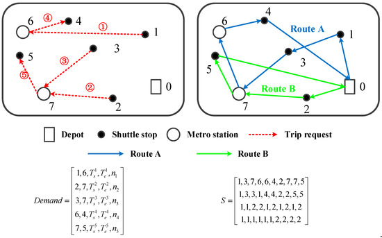
Figure 1.
An example of the study area, trip requests and vehicle routes.
Some basic assumptions are made as follows:
- The vehicle travel time between every two stops/stations and the dwell time at the stops/stations are assumed to be constants.
- The requests are performed by a set of routes equipped with homogeneous vehicles.
- The requested time window refers to the time window of the pickup service in this study, and the delivery time window is considered as the maximum allowable in-vehicle time.
2.2. Objective Function
The objective function of this study mainly consists of the passenger in-vehicle cost and the operator cost. It can be written as follows.
where CT is the total cost, which includes both the operator cost and the passengers’ in-vehicle cost. CS is the operator cost, which is related to the set of designed routes (S) and can be further expressed as (2), and CI is the passenger in-vehicle cost, which is related to both S and the set of vehicle departure time (denoted by D0) and is further expressed as (3).
where is the vehicle travel time between every two adjacent stops on route r, is the arrival time at stop i on route r, is the service start time at stop i on route r, nk is the number of passengers of request k. δ1 (r, k, i) and δ2 (r, k, i) are binary variables that equal 1 if stop i on route r is the starting and terminal stop of request k and equal 0 otherwise, is the operator cost per unit of distance, and is the passenger cost per unit of in-vehicle time.
For i and r, there exist some relationships among the vehicle arrival time (), the service start time (), and the vehicle departure time (denoted by ). The vehicle arrival time at a stop can be expressed as the departure time at the last stop plus the travel time between the two stops. The vehicle departure time at a stop can be further expressed as the service start time plus a dwell time at the stop (which is assumed as a constant and denoted by ts). The service start time values the vehicle arrival time if the vehicle arrives no earlier than the lower limit of the service time window, which is denoted by (r, i-the index indicating the route and the stop), otherwise, it will wait until .
2.3. Constraints
The constraints of the problem are formulated as follows.
For a pickup service, Constraint (4) is the time window constraint formulated by collecting the submitted information of each request, where and are the lower and upper limits of a service time window, |r| is the number of stops (except the depot) on route r. It is worth noting that for a delivery service, Constraint (4) becomes the maximum in-vehicle delay constraint of each request. To combine the two constraints together, we define Constraint (4) as service time window constraint, where the service includes both the pickup service and the delivery service. For a pickup service, the time window is given by the request, while for a delivery service, and are automatically generated by adding and λ based on them where denotes the least in-vehicle time of request k and λ is a coefficient greater than 1.
Constraint (5) is the vehicle capacity constraint which restricts the loading on any segment () not exceed the vehicle capacity (P). Constraint (6) is the route duration constraint, where , , denote the vehicle departure time at the depot, departure time at the last stop and the travel time between the last stop and the depot, respectively. Constraints (7)–(8) ensure that each request is performed by a vehicle once. Constraint (9) restricts that the start and the terminal stop of each request are visited by the same vehicle.
In this study, Constraints (7)–(9) are satisfied by the designed metaheuristics and the internal operators that will be described in Section 4 and Section 5. Constraints (4)–(6) are treated as soft constraints and three types of penalties are formulated, accordingly.
where CP1, CP2, CP3 are the penalties incurred by the violations of the service time window constraint, the vehicle capacity constraint, and the route duration constraint. g1(x), g2(x), g3(x) are the corresponding penalty functions with respect to the service start time, the segment loading and the route duration. Combined with the optimal departure time determination method that will be described in Section 3, we believe that a more competitive solution can be obtained by the treatment.
By adding the three penalties into the original objective function, the new objective can be written as follows.
3. Vehicle Departure Time Determination
For a route serving m trip requests, let be the set of pickup service nodes and and be the sets of lower limits and upper limits of the corresponding time windows, respectively. For each , the speculated vehicle departure time at the depot (denoted by ) is a critical departure time that makes the slack time at iu be 0. This means that a synchronization delay at iu caused by the delay at the depot occurs only when the vehicle departs later than . Similarly, for , the speculated departure time at the depot is denoted by . can be treated as another critical departure time that makes the time window penalty at iu be 0, and the penalty is greater than 0 if the vehicle departs later than this time.
Let and store the vehicle departure time that is speculated using all the elements in and , respectively. Two propositions are presented as follows:
Proposition 1.
For, there always exists.
Proposition 2.
Forand, if,,,,, anddo not change with, otherwise,, andare positively correlated with, and there exists.
Before analyzing the impact of on each cost and penalty, we first divide Cp1 in (10) into two parts: the time window penalty due to the pickup service delay (denoted by Cp11) and the one due to the delivery service delay (denoted by Cp12). The division is motivated by the fact that has different impacts on the two types of penalties. As we analyzed above, when gradually increases within the time horizon, Cp11 first remains stable and then increases with a growing slope since increasingly more values in are exceeded by . In contrast, Cp12 decreases in this process and finally becomes stable since it is determined by the total passengers’ in-vehicle time. In addition, CI and CP3 have a similar trend with Cp12 as increases. A quantified analysis is illustrated as follows.
3.1. Impact of on CI and Cp12
Assume that the request k is performed by route r, where its pickup and delivery nodes are denoted by ik1 and ik2, respectively. The in-vehicle cost (denoted by ) and the time window penalty of delivery service (denoted by ) of the request k are expressed as follows.
Let in be the last pickup node between ik1 and ik2 if there exists one. Let be the speculated departure time at the depot using the lower limit of the time window of in. From propositions 1–2, is the maximum departure time that prevents Aik2 from increasing with increasing . Similarly, , which is the speculated departure time at the depot using the lower limit of the time window of ik1, is the maximum departure time that prevents Bik1 from increasing with increasing . That is, when increases within , Bik1 increases synchronously while Aik2 remains unchanged. Therefore, linearly decreases with increasing , and we have from propositions 2. Based on the analysis, the first derivatives of and with respect to are obtained by Equations (16) and (17), respectively.
The impact of on the sum of and of all the requests on route r can be obtained by Equation (18).
3.2. Impact of on Cp11
For the request k performed by route r, the time window penalty of pickup service (denoted by ) is expressed by Equation (19).
Let be the speculated departure time at the depot using the upper limit of the time window of ik1. We can conclude that Bik1 increases with increasing and is always greater than if . That is, is the maximum departure time that prevents from increasing with increasing . Combined with proposition 2, it is clear that and . Therefore, the first derivative of with respect to is obtained by Equation (20).
For all the requests performed by route r, the impact of on the sum of can be expressed as Equation (21).
3.3. Impact of on Cp3
For a route r that performs m requests, let be the departure time at the last service node, and let be the travel time from the last service node to the depot, then, the route duration of r can be written as . The route duration penalty of r is expressed as follows.
Similar to the impact on , the impact on is determined by a critical departure time , which represents the speculated departure time at the depot using the lower limit of the time window of the last pickup service node on r. Therefore, the first derivative of with respect to is expressed as follows.
The derivative of the total cost on route r with respect to (denoted by ) is determined by accumulating the three derivatives above (Equations (18), (21), (23)). Then, we seek all the extreme points of that make to formulate the set of candidate departure times. The optimal departure time is then determined by choosing the departure time with the minimum total cost (including penalties).
4. Solution Framework
4.1. Initial Route Generation
As stated above, the constraints of the time window, vehicle capacity, and route duration are modeled as soft constraints. In the solution generation stage, we need only to ensure that the pickup and delivery nodes of each request are sequentially performed once by the same route.
To generate an initial solution, we first sort all the requests in ascending order according to and assign the first R requests to each route directly, where R is the number of routes. Then, we assign the following requests to a certain route in sequence according to a set of probabilities. Assuming that request k’ is the current last request on route r, the probability of adding request k () to route r is related to three items: the spatial distance between the delivery stop of k’ and the pickup stop of k (denoted by ), the temporal distance between k and k’ (denoted by and defined by Equation (25)), the current number of nodes on r (denoted by ). The probability is obtained by Equation (24).
where is the probability of adding request k to route r, , , and are coefficients.
4.2. Request Insert Operator
The request insert is a basic operator that is repeatedly called by the following sequence reorder operator and meta-heuristics to ensure that the solution is feasible. To insert an unperformed request into a current route, the operator selects two positions on the route to insert the pickup node and service node with the aim of saving the cost increment as much as possible. To this end, two insert operators, which are denoted by DI1and DI2, are developed. DI1 determines the positions exactly by enumerating all possible insertion cases, while DI2 first determines the pickup position by a certain method and then enumerates all possible delivery positions. The steps of the two operators are given in Algorithm 1 and Algorithm 2.
| Algorithm 1. Request Insert-1 (DI1). |
|
| Algorithm 2. Request Insert-2 (DI2). |
|
From Algorithm 1 and Algorithm 2, it is clear that DI1 obtains the best pair of insert positions exactly by times of attempts. By using DI2, this number can be reduced to , however, the obtained pair of positions may not as good as the pair obtained by DI1.
4.3. Sequence Recorder Operator
When all the requests are assigned to a certain route, the sequence reorder operator is applied to optimize the performance sequence on each route. Two sequence reorder operators, which are denoted by L1 and L2, are developed here. The steps are given in Algorithm 3 and Algorithm 4.
| Algorithm 3. Sequence Reorder-1 (L1). |
|
| Algorithm 4. Sequence Reorder-2 (L2). |
|
Comparing Algorithm 3 and Algorithm 4, the input of L1 includes both the route (i.e., the current performance sequence of requested service) and the requests, while L2 needs to input only the set of requests. Assuming the number of requests in to be , it is clear that the request insert operator is performed times by both L1 and L2. However, the detailed runs of L1 and L2 are still different since the lengths of routes to be inserted are different each time in L1 and L2. Table 1 gives the runs of calculations by different combinations of DI1, DI2, L1, and L2.

Table 1.
Runs of calculations by different combinations of DI1, DI2, L1, and L2.
4.4. Tabu Search
The tabu search (TS) algorithm starts from the initial solution and generates a new nontabu solution in each iteration. The new solution is generated based on the current one by a developed neighborhood search mechanism. To avoid searching cyclically, a tabu list is established to record some attributes of recently visited solutions. A newly generated solution that possesses the attributes is declared forbidden. In this study, we use the tabu scheme to prevent a request to be reinserted into the route that it was just removed from recently. After a number of iterations, the forbiddance will be released to maintain the stability of the size of the neighborhood solution space.
The neighborhood solution is obtained by transferring a certain request from its original route to another route obeying the tabu list. The request to be transferred each time is selected by a probability, which is expressed as follows.
where is the total cost after removing request k, is the number of passengers for request k.
Similarly, the route that the request is transferred to is also selected according to a certain probability, which is written as Equation (27). It shows that the probability is determined only by the current route length.
Let Demand be the set of requests, S0, CT0, and D00 are the initial solution, the corresponding total cost and set of departure times, respectively. S*, and are the obtained best solution, the minimum total cost and the corresponding set of departure time. θ is the number of iterations that a forbiddance is released. Tabu is the tabu list. P_Tabu is the matrix that records the number of iterations each forbiddance lasts. MAXGEN is the maximum number of iterations, and is the number of iterations between two adjacent performances of sequence reordering. The detailed steps of the TS are described in Algorithm 5.
| Algorithm 5. Tabu Search (TS). |
|
4.5. Variable Neighborhood Search
A variable neighborhood search algorithm that includes two types of neighborhood search methods is developed to diversify the neighborhood solution space. In the first method, two routes are selected to perform the cross-exchange/transfer of certain requests. An example of the method is presented in Figure 2, in which each cycle represents a request. The number of requests selected on each route to perform the cross-exchange/transfer is denoted by cn1.
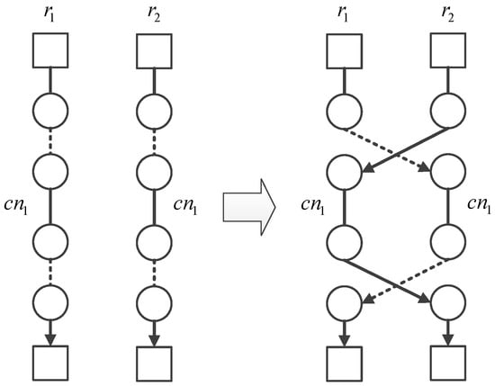
Figure 2.
A cross-exchange/transfer of requests between two routes.
It is worth noting that to make the operation be carried out smoothly, at least one of the two routes needs to perform more than cn1 requests. If the number of requests on both of the routes exceeds cn1 and the difference between the two individual counts is no more than a preset threshold denoted by Δl, a cross-exchange of cn1 requests is performed between the two routes. Otherwise, we select only cn1 requests from the route with more requests and transfer them to the other one. The requests are still selected according to the set of probabilities defined by (26). Then, DI1 or DI2 are performed to shift the requests to the other route.
The second neighborhood search is proposed to make a cyclic transfer of requests among multiple routes, which is also proposed in Reference [24] to solve the vehicle routing problem. An example of the method is presented in Figure 3, in which cm2 and cn2 respectively denote the number of routes and requests to participate in the transfer. Before the request transfer process, we first sort the routes in descending order according to the route length (i.e., the number of requests). To make the method be conducted smoothly, the number of requests on route r1 should exceed cn2. Moreover, if the difference between the numbers of requests performed by the first and the last routes exceeds the threshold Δl, the process terminates by completing the requested transfer from the second to last route to the last one. Otherwise, it performs one additional transfer, i.e., the transfer from the last route to the first one. Compared with the request transfer scheme presented in Figure 2, this transfer method shows the ability to provide larger neighborhood solutions due to the participation of more than two routes.
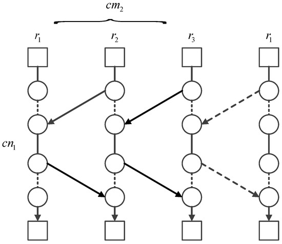
Figure 3.
A cyclic transfer of requests among multiple routes.
To further diversity the neighborhood solution space, we replace the original parameters cn1, cm2, and cn2 with three new parameters: cn1max, cm2max, and cn2max, which denote the preset maximum values of the original parameters. In each performance of the neighborhood search methods, cn1, cm2, and cn2 are randomly generated according to cn1max, cm2max, and cn2max. In this study, we attempt to set cn1max from 1 to 3, set cm2max from 3 to 4, and set cn2max from 1 to 3. Therefore, at most 9 attempts of neighborhood search are performed in each iteration. The parameters are sequentially listed as follows: cn1max ← 1 ⇨ cn1max ← 2 ⇨ cn1max ← 3 ⇨ cm2max ← 3, cn2max ← 1 ⇨ cm2max ← 3, cn2max ← 2 ⇨ cm2max ← 3, cn2max ← 3 ⇨ cm2max ← 4, cn2max ← 1 ⇨ cm2max ← 4, cn2max ← 2 ⇨ cm2max ← 4, cn2max ← 3. The former 3 attempts to use the cross-exchange/transfer method, while the latter 6 attempts are based on the cyclic-transfer method. If the solution obtained by an attempt to search is better than the current one, the process breaks immediately. Otherwise, we choose the best solution from the 9 obtained solutions and check whether it replaces the current solution by the acceptance criterion of the simulated annealing. The detailed steps are given in Algorithm 6. For the meanings of some repeated notations, one can refer to Algorithm 5, we do not repeat them here.
| Algorithm 6. Variable Neighborhood Search (VNS). |
Return to Step 5. |
5. Case Study
The network of the study area is the Huilongguan Community, which is large in size (about 4.8 km 2.2 km) and located in Beijing, China. As shown in Figure 4, there are 52 bus stops (Nodes 1–52), 6 metro stations (Nodes 53–58) and a depot (Node 0) in the area. By connecting the pairs of the nodes that no other stops exist on the shortest path between them, we formulate the corresponding topology network which is presented in Figure 5.
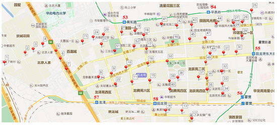
Figure 4.
The network, bus stops and metro stations of Huilonguan Community.
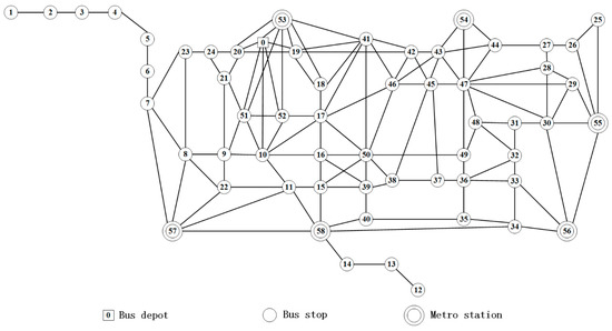
Figure 5.
The topological structure of the network of Huilonguan Community.
To simulate the process of generating a trip request, we first randomly choose two nodes from Nodes 1–52 and 53–58 as the origin and the destination since each trip request in the study is defined between a bus stop and a metro station. To generate the reversed trip requests which start from a metro station and terminate at a bus stop, the origin and the destination are just needed to be exchanged according to a certain probability, which can be understood as the ratio of the bidirectional trip requests. Here we set the probability as 0.7. That is if the randomly generated number between 0 and 1 after generating a trip request is greater than 0.7, we exchange the origin and the destination. To randomly generate the time window and the number of passengers, some parameters are set as follows: the time horizon LN = 300 min, the range of the pickup time window obeys the normal distribution N (10, 22), and the maximum number of passengers per request is set as DNmax = 5. We repeat the generation process to randomly generate 100 requests and formulate the matrix Demand by sorting them in ascending order according to .
The other parameters are set as follows: R = 5, ts = 0.5 min, = 9 RMB/min, = 1 RMB/min, λ = 1.5, P = 11, and Tmax = 180 min. The penalty functions g1(x), g2(x), and g3(x) are defined by Equations (28)–(30).
In the TS algorithm, θ = 30, MAXGEN = 300, and = 10. In the VNS algorithm, T0 = 3000, Tend = 0.001, q = 0.96, Δl = 22, and = 10. The results presented below are obtained by using MATLAB 2015a on a personal computer with Intel Core i5-3230 CPU @2.6GHz.
Based on the preset parameters above, 4 sets of experiments (represented by DI1+L1, DI1+L2, DI2+L1, and DI2+L2) with different combinations of internal operators are designed to test the TS performance of each case. The convergence processes of the 4 cases are presented in Figure 6. Some related results are given in Table 2.
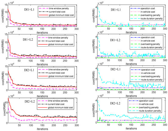
Figure 6.
Evolving curves of each experiment by using a tabu search (TS).
Table 2.
Detailed results and CPU time of each experiment by using TS.
In Figure 6, the results of each set are presented in two subfigures so that the optimization process of each cost or penalty is presented clearly. In each pair of subfigures of each set, the penalties of the service time window and the route duration take up most of the total cost within the about first 50 iterations. After that, the curves of these two items decrease sharply so that the infeasible solutions with serious violations of the constraints are ensured to be eliminated. Due to the parameters we set, the remaining three items, i.e. the operation cost, the in-vehicle cost, and the overloading penalty account for a small portion of the total cost and keep relatively stable in the whole optimization process. From the left subfigures, it is clear to see that the curves of the global minimum total costs of the 4 cases remain stable after approximately 50 iterations. However, minor fluctuations always exist on the curves of the current total costs even in late iterative processes, especially for the last three sets, i.e. the sets of DI1+L2, DI2+L1, DI2+L2. Therefore, it seems that we may obtain a satisfactory solution fast by using the TS, but the algorithm also shows an inadequate ability in providing continuous improvements in the late iteration process.
In Table 2, the case of DI1+L1 obtains the solution with the lowest objective value, however, it is also the most time-consuming case. Conversely, another extreme performance with the worst solution and the least CPU time occurs in the case of DI2+L2. The results of CT do not differ much between the cases of DI1+L1 and DI1+L2. However, DI1+L2 saves more than half of the CPU time compared with DI1+L1. This indicates that the use of L2 may also lead to a good solution with much higher efficiency. A much worse solution may be obtained if we use DI2 instead of DI1, which can be confirmed by comparing the former two cases in Table 2 with the latter two ones.
To test the performance of the VNS, 4 sets of experiments with the same combinations of internal operators in the VNS framework are conducted. The evolving processes are presented in Figure 7 where each set is also presented by two subfigures, and the related results are given in Table 3.
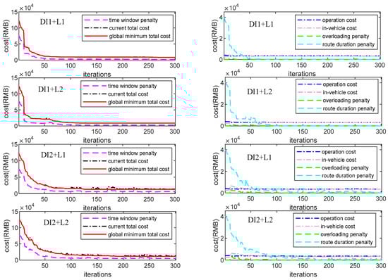
Figure 7.
Evolving curves of each experiment by using variable neighborhood search (VNS).
Table 3.
Detailed results and CPU time of each experiment by using VNS.
In each pair of subfigures of Figure 7, the penalties of the service time window and the route duration still take up most of the total cost and decrease sharply at the start of the evolving process. In contrast, the curves of the remaining three items keep stable with relatively small values in the whole process. Comparing the curves in Figure 7 with the ones in Figure 6, it is clear that the curves of almost all the items in Figure 7 are more stable with fewer fluctuations, although the global minimum total costs converge slightly slower (approximately within 70 iterations). In particular, in the case of DI1+L1 by using the VNS, the curves of the global minimum total cost and the current total cost are completely coincident. This confirms the effectiveness of the VNS since the current solution is constantly optimized as the iteration processes.
The results in Table 3 indicate similar conclusions about the performance of the four cases, as shown in Table 2. However, the objective values here are less than the ones in Table 2 for all four cases, especially for the latter two cases. By comparing the two tables, the percentages of the total cost reduction in Table 3 are found to be 21.4%, 20.6%, 32.6%, and 57.5%. On the other hand, the VNS costs more CPU time in general. The percentages of the CPU time increase by using VNS are 166.1%, 198.6%, 30.6%, and 32.0%. Therefore, we conclude that DI2 is well suited to the VNS framework since the latter two cases in Table 3 provide much better solutions than the corresponding ones in Table 2 without much CPU time consumption. Moreover, the VNS solutions are less influenced by different combinations of the internal operators than the other solutions since the objective values of the four cases in Table 3 do not differ significantly. However, the VNS seems to be more sensitive from the perspective of CPU time.
To evaluate the performances of the TS and the VNS more comprehensively, 15 sets of experiments (represented by 1a~5c) with different problem scales and time windows are conducted. The number of requests in cases 1~5 are set as 60, 80, 100, 120, and 140. The time windows in subcases a~c are randomly generated based on the normal distribution N (5, 12), N (10, 22), and N (15, 32). Both the TS and the VNS with DI1+L2 are used to solve the 15 sets of problems 5 times. The minimum objective value (denoted by and ), the average objective values (denoted by and ), and the CPU time of the 5 runs by using the TS and VNS of each case are recorded in Table 4. In addition, the percentage of differences between and (denoted by and , respectively) solved by the TS and VNS in each case are also given in Table 4.
Table 4.
Comparison of the results obtained by TS and VNS in each case.
In Table 4, the CPU time by using each meta-heuristic has a remarkable growth from case 1 to case 5 as the problem scale increases. For each case from case 1 to case 5, the minimum objective values and the average values obtained by the two meta-heuristics both decreases from subcase a to subcase c in general since the intensity of the time window constraint becomes weaker as the time window width increases. Comparing the performances of the TS and VNS, the VNS obtains a better solution in each of the 15 experiments, which can be confirmed by the negative values of and in each case. Moreover, the difference between the objective values obtained by the two meta-heuristics increases as the problem scale increases. For the problems with 60 requests (case 1a~1c), and are approximately 10%. For the problems with 140 requests (case 5a~5c), the values increase to 30~40%. Therefore, a much better solution may be obtained by the VNS for a large-scale problem. However, the CPU time of the VNS also increases sharply as the problem scale increases. For example, it is found to increase by 4353.9 sec by comparing case 1a with case 5a, while the CPU time of the TS increases by only 1715.8 sec. This suggests that making a trade-off between the solution quality and CPU time consumption is critical when solving a large-scale problem in practice.
6. Conclusions
This paper optimizes the routes and the vehicle departure times of community shuttles based on demand-responsive service. By considering the constraints of the time window, vehicle capacity and route duration as soft constraints, an analytical method of determining the vehicle departure time is developed to obtain a competitive solution that can be effectively used in real-world operations. To solve the routing problem, a tabu search (TS) and a variable neighborhood search (VNS) with multiple internal operators are designed. Finally, a case study is presented to test the algorithms followed by analysis. The key conclusions are summarized as follows:
Both the TS and the VNS with different combinations of internal operators provide clear convergence trends within 100 iterations during the evolving process. The curves of the VNS converge slightly slower but are more stable than those of the TS in general. Of the two, the VNS usually obtains a better solution with more CPU time consumption. The gaps in the objective value and the CPU time by using the two metaheuristics widen as the problem scale increases. In the 15 sets of experiments with different numbers of requests and time window widths, the percentage differences of objective values vary from less than 10% to more than 30% as the number of requests increases from 60 to 140. However, the difference in the CPU time also increases sharply in this process.
Two request insert operators (i.e., DI1 and DI2), as well as two sequence reorder operators (i.e., L1 and L2), are developed. DI1 and L1 are used to improve the solutions through additional runs. Therefore, ‘DI1+ DI1’ provides the best solution with the most CPU time, while ‘DI2+ DI2’ is the opposite extreme case. In the experiments involving both the TS and the VNS, L2 is found to be a competitive sequence reorder operator that leads to good solutions with much higher efficiency than L1. In contrast, DI2 is more suitable than DI1 for the VNS framework. From the perspective of solution quality, of the two metaheuristics, the VNS is less influenced by different combinations of the internal operators. However, it is more sensitive from the view of CPU time.
As described above, the model includes an analytical method to determine the optimal vehicle departure time by treating the related constraints as soft constraints. Undoubtedly, the departure time solution is greatly affected by the penalty functions and it may not be effectively used into practice if the relevant parameters are not well calibrated. Besides, the model is developed with a given number of routes. However, the shuttle operators are usually more sensitive to the fleet size of the vehicles they can invest rather than the number of routes. Therefore, future research could be performed by relaxing the preset number of routes and replacing this parameter with a fleet size constraint. This step would result in a jointly optimal design problem of routing and vehicle scheduling. By solving the problem effectively, some relationships among the trip requests, number of routes, departure time, and fleet size could be further explored.
Author Contributions
Conceptualization, J.X. and B.C.; methodology, J.X.; formal analysis, J.X.; investigation, B.C.; writing—original draft preparation, B.C. and X.L. writing—review and editing, J.X. and Z.H.; supervision, Y.C.; funding acquisition, J.X. All authors have read and agreed to the published version of the manuscript.
Funding
This research is sponsored by National Key Research and Development Program of China (2018YFB1601300), National Natural Science Foundation of China (71601006), Science and Technology Development Foundation of Beijing Municipal Education Commission (KM201710005030).
Conflicts of Interest
The authors declare no conflict of interest.
References
- He, Z.; Zheng, L.; Chen, P.; Guan, W. Mapping to Cells: A Simple Method to Extract Traffic Dynamics from Probe Vehicle Data. Comput. Civ. Infrastruct. Eng. 2017, 32, 252–267. [Google Scholar] [CrossRef]
- Jiang, S.; Guan, W.; He, Z.; Yang, L. Measuring Taxi Accessibility Using Grid-Based Method with Trajectory Data. Sustainability 2018, 10, 3187. [Google Scholar] [CrossRef]
- Dong, H.; Wu, M.; Ding, X.; Chu, L.; Jia, L.; Qin, Y.; Zhou, X. Traffic zone division based on big data from mobile phone base stations. Transp. Res. Part C: Emerg. Technol. 2015, 58, 278–291. [Google Scholar] [CrossRef]
- Xiong, J.; Guan, W.; Song, L.; Huang, A.; Shao, C. Optimal Routing Design of a Community Shuttle for Metro Stations. J. Transp. Eng. 2013, 139, 1211–1223. [Google Scholar] [CrossRef]
- Xiong, J.; He, Z.; Guan, W.; Ran, B. Optimal timetable development for community shuttle network with metro stations. Transp. Res. Part C: Emerg. Technol. 2015, 60, 540–565. [Google Scholar] [CrossRef]
- Xiong, J.; Chen, B.; Chen, Y.; Jiang, Y.; Lu, Y. Route Network Design of Community Shuttle for Metro Stations Through Genetic Algorithm Optimization. IEEE Access 2019, 7, 53812–53822. [Google Scholar] [CrossRef]
- Amirgholy, M.; Gonzales, E.J. Demand responsive transit systems with time-dependent demand: User equilibrium, system optimum, and management strategy. Transp. Res. Part B: Methodol. 2016, 92, 234–252. [Google Scholar] [CrossRef]
- Agatz, N.; Erera, A.; Savelsbergh, M.; Wang, X. Optimization for dynamic ride-sharing: A review. Eur. J. Oper. Res. 2012, 223, 295–303. [Google Scholar] [CrossRef]
- Ho, S.C.; Szeto, W.; Kuo, Y.-H.; Leung, J.M.; Petering, M.; Tou, T.W. A survey of dial-a-ride problems: Literature review and recent developments. Transp. Res. Part B: Methodol. 2018, 111, 395–421. [Google Scholar] [CrossRef]
- Røpke, S.; Pisinger, D. An Adaptive Large Neighborhood Search Heuristic for the Pickup and Delivery Problem with Time Windows. Transp. Sci. 2006, 40, 455–472. [Google Scholar] [CrossRef]
- Røpke, S.; Cordeau, J.-F. Branch and Cut and Price for the Pickup and Delivery Problem with Time Windows. Transp. Sci. 2009, 43, 267–286. [Google Scholar] [CrossRef]
- Irnich, S. A multi-depot pickup and delivery problem with a single hub and heterogeneous vehicles. Eur. J. Oper. Res. 2000, 122, 310–328. [Google Scholar] [CrossRef]
- Landrieu, A.; Mati, Y.; Binder, Z. A tabu search heuristic for the single vehicle pickup and delivery problem with time windows. J. Intell. Manuf. 2001, 12, 497–508. [Google Scholar] [CrossRef]
- Naccache, S.; Côté, J.-F.; Coelho, L.C. The multi-pickup and delivery problem with time windows. Eur. J. Oper. Res. 2018, 269, 353–362. [Google Scholar] [CrossRef]
- Haddad, M.N.; Martinelli, R.; Vidal, T.; Martins, S.; Ochi, L.S.; Souza, M.J.F.; Hartl, R. Large neighborhood-based metaheuristic and branch-and-price for the pickup and delivery problem with split loads. Eur. J. Oper. Res. 2018, 270, 1014–1027. [Google Scholar] [CrossRef]
- Qu, Y.; Bard, J.F. The heterogeneous pickup and delivery problem with configurable vehicle capacity. Transp. Res. Part C Emerg. Technol. 2013, 32, 1–20. [Google Scholar] [CrossRef]
- Masson, R.; Lehuédé, F.; Péton, O. The Dial-A-Ride Problem with Transfers. Comput. Oper. Res. 2014, 41, 12–23. [Google Scholar] [CrossRef]
- Reinhardt, L.B.; Clausen, T.; Pisinger, D. Synchronized dial-a-ride transportation of disabled passengers at airports. Eur. J. Oper. Res. 2013, 225, 106–117. [Google Scholar] [CrossRef]
- Detti, P.; Papalini, F.; De Lara, G.Z.M. A multi-depot dial-a-ride problem with heterogeneous vehicles and compatibility constraints in healthcare. Omega 2017, 70, 1–14. [Google Scholar] [CrossRef]
- Tong, L.; Zhou, L.; Liu, J.; Zhou, X. Customized bus service design for jointly optimizing passenger-to-vehicle assignment and vehicle routing. Transp. Res. Part C: Emerg. Technol 2017, 85, 451–475. [Google Scholar] [CrossRef]
- Braekers, K.; Caris, A.; Janssens, G.K. Exact and meta-heuristic approach for a general heterogeneous dial-a-ride problem with multiple depots. Transp. Res. Part B Methodol. 2014, 67, 166–186. [Google Scholar] [CrossRef]
- Parragh, S.N.; Schmid, V. Hybrid column generation and large neighborhood search for the dial-a-ride problem. Comput. Oper. Res. 2013, 40, 490–497. [Google Scholar] [CrossRef] [PubMed]
- Parragh, S.N.; Doerner, K.F.; Hartl, R.F. Variable neighborhood search for the dial-a-ride problem. Comput. Oper. Res. 2010, 37, 1129–1138. [Google Scholar] [CrossRef]
- Ibaraki, T.; Imahori, S.; Kubo, M.; Masuda, T.; Uno, T.; Yagiura, M. Effective Local Search Algorithms for Routing and Scheduling Problems with General Time-Window Constraints. Transp. Sci. 2005, 39, 206–232. [Google Scholar] [CrossRef]
© 2020 by the authors. Licensee MDPI, Basel, Switzerland. This article is an open access article distributed under the terms and conditions of the Creative Commons Attribution (CC BY) license (http://creativecommons.org/licenses/by/4.0/).