Spatially Explicit Mapping of Historical Population Density with Random Forest Regression: A Case Study of Gansu Province, China, in 1820 and 2000

Abstract

This study established a random forest regression model (RFRM) using terrain factors, climatic and river factors, distances to the capitals of provinces, prefectures (Fu, in Chinese Pinyin), and counties as independent variables to predict the population density. Then, using the RFRM, we explicitly reconstructed the spatial distribution of the population density of Gansu Province, China, in 1820 and 2000, at a resolution of 10 by 10 km. By comparing the explicit reconstruction with census data at the township level from 2000, we found that the RFRM-based approach mostly reproduced the spatial variability in the population density, with a determination coefficient (R²) of 0.82, a positive reduction of error (RE, 0.72) and a coefficient of efficiency (CE) of 0.65. The RFRM-based reconstructions show that the population of Gansu Province in 1820 was mostly distributed in the Lanzhou, Gongchang, Pingliang, Qinzhou, Qingyang, and Ningxia prefecture. The macro-spatial pattern of the population density in 2000 kept approximately similar with that in 1820. However, fine differences could be found. The 79.92% of the population growth of Gansu Province from 1820 to 2000 occurred in areas lower than 2500 m. As a result, the population weighting in the areas above 2500 m was ~9% in 1820 while it was greater than 14% in 2000. Moreover, in comparison to 1820, the population density intensified in Lanzhou, Xining, Yinchuan, Baiyin, Linxia, and Tianshui, while it weakened in Gongchang, Qingyang, Ganzhou, and Suzhou.

1. Introduction

The spatial distribution of populations is one of the hot topics in the field of demography. With the introduction of geography and statistics, the spatial distribution of populations has gradually become a complex, multidisciplinary research problem [1,2,3]. However, most of the demographic datasets were compiled based on administrative districts such as counties and townships. As a consequence, it has been impossible to depict the spatial variability in the population density within the administrative areas. This lack of knowledge leads to some limitations on many relevant issues, such as interactions of humans and the environment, because many natural environmental factors have explicit spatial variability [4]. The estimated population distribution can provide more spatial detailed information of population with regular grid cells and can be used to reveal the pattern of population growth and migration [5]. Furthermore, the gridded historical population datasets are widely used in the historical reconstruction of land use and land cover change (LUCC), such as the conversion from woodland to cropland, which is conducive to the quantitative estimations of carbon emissions in historical periods [6,7,8]. Therefore, there has been a large demand to determine the explicit spatial distribution of population.

To date, there are a large number of global- and national-scale gridded population datasets including the Gridded Population of the World (GPW), Global Rural-Urban Mapping Project (GRUMP), WorldPop datasets, and China 1 km Gridded Population (CnPop) datasets [9]. These datasets played critical roles in resource allocation and management [10], climate change research [11,12], disease risk assessment [13], and other fields. These existing studies mostly focused on modern times; however, there are a few population gridded datasets for historical periods. This may be partly explained by the lack of documented historical census data.

Overall, the modelling approaches of most population gridded datasets can be divided into two categories: a spatial interpolation (SITP) approach and multi-factor integration (MFI) approach. The SITP approach is based on geo-statistics. Under the SITP approach, population density is represented as a function of location, i.e., the X-coordinate and Y-coordinate [14]. To quantify the relationship between population density and locations, many models such as the inverse distance weighted model, kriging model, spline model, and natural neighbor model have been applied [15]. Using observations, the models are calibrated; then, they are used to calculate the population density of the sites without observations. Hence, the SITP approach assumes that the positions (distance) of the sampling points are dominant factors determining the population distribution but do not explicitly represent the impacts of environmental factors on the population distribution. SITP is usually used to transform irregular population density sampling points into rasters in situations lacking environmental factors. However, due to the limitations of the SITP approach, the population near the sampling points is usually overestimated, which is inconsistent with the actual population distribution.

The MFI approach is usually based on a multiple variable regression. Using the MFI approach, the population density is represented as a function of multiple environmental factors including altitude, slope, river, night-time light strength, land cover/use proportions, and satellite-based vegetation indexes [16,17,18,19]. Typically, a linear multiple variable regression is applied to quantify the relations between the population density and environmental factors. The regression model is calibrated with the observations; then, it is used to estimate the population density of sites with environmental variables but missing population observations. In comparison with the abovementioned SITP approach, the MFI approach considers the environmental factors closely related to population density, rather than only location and distance. Therefore, the MFI approach has been used extensively to construct the explicit spatial distribution of population density in recent decades [20,21]. However, the MFI approach usually requires a large number of independent variables, most of which are unavailable for the historical periods. Moreover, a traditional linear regression cannot describe the complex relationship between the population density and environmental factors. Therefore, the existing MFI approach is rarely applied to reconstruct the explicit spatial distribution of population density for historical periods.

Recently, intelligent algorithms were applied to establish the relationship between populations and environmental factors and simulate the population distribution in grid cells [22]. The most widely used intelligent algorithms for population spatialization is the random forest regression model (RFRM). The RFRM is an integrated learning method based on an ensemble of a large set of decision trees [23]. Some studies have shown that the RFRM can explain the nonlinear relationship between independent variables and dependent variables better than a conventional regression model [24,25,26]. It is noted that the existing study with RFRM used a large number of environmental factors as the independent variables. However, there are differences in the environmental factors between the historical period and present day. For example, the cities are densely populated areas from ancient times to now, after the industrial revolution, the cities had more attractions for the population than in its ancient period. Some studies showed that historical population distribution was partly dependent on the political situation and climate change [27,28]. In addition, environmental factors such as land use proportions and night-time light intensity are unavailable for the historical period. Thus, it still remains unclear if the RFRM could be applied to modelling population distribution with very limited environmental factors for the historical period.

China has a long history of recording census data, and the earliest census data can be traced back to 2 AD. However, all of these data were based on censuses conducted in political units, and as a result, the explicit spatial distribution of the population remains unclear. Currently, only few studies have attempted to reconstruct the explicit spatial distribution of populations in historical periods of China. For instance, Wang et al. [29] simulated the population distribution of China in the Western Han Dynasty (202 BC–8 AD) with the SITP approach. Therefore, the spatially explicit distributions of the populations in historical period in China needed to be reconstructed.

In this paper, the RFRM was used to model population density with few available environmental factors in grid cells with a size of 10 by 10 km, and Gansu Province, China, in 1820 and 2000 was used as the case study.

2. Materials and Methods

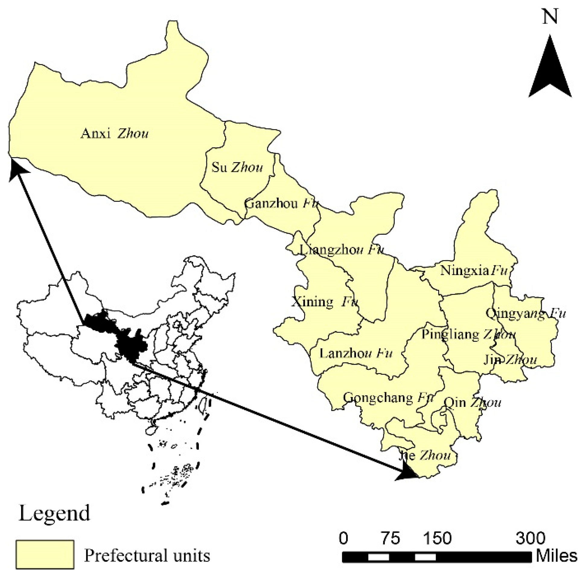
2.1. Study Area

The study area was Gansu Province, China, in 1820, during the Qing Dynasty. The area of Gansu Province was slightly larger in 1820 than it is at present. It not only included present-day Gansu Province but also present-day Ningxia and a small portion of Qing Hai. There were 13 prefectural units (Fu) including Lanzhou, Pingliang, Gongchang, Xining, Ningxia, etc. (Figure 1). The region is located in the junction of the Loess Plateau, the Qinghai-Tibet Plateau, and the Inner Mongolia Plateau. The terrain of the area is high in the west and south and low in the east and north. It is dominated by a temperate monsoon climate, which is characterized by cold and dry winters and warm and moist summers.

Gansu Province is the key area of the ancient Silk Road. With the development of commerce and trade, many cities (i.e., Lanzhou, Liangzhou, Ganzhou, and Dunhuang) were regarded as transportation hubs in the ancient period. The development of the cities further led to the uneven distribution of the population in this area. Thus, we need to reconstruct the population distribution in Gansu Province, and it may be of great significance to study human–environment interactions and the evolution of civilization [30].

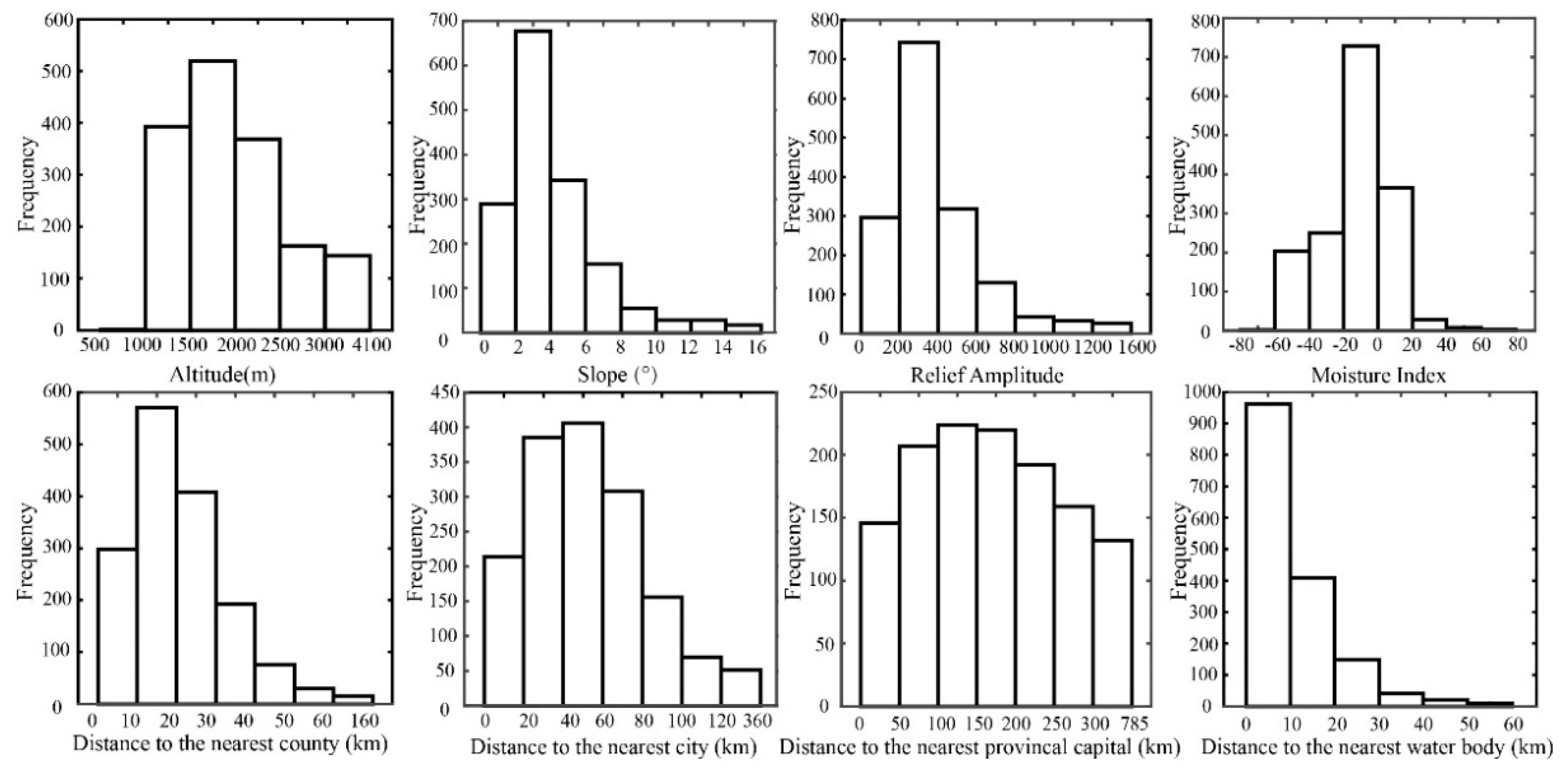
2.2. Environment Factors and Data Resources

Existing studies show that population density is determined by many factors [31,32]. These factors are essentially classified into two categories: natural factors and human factors. Based on existing studies together with the availability of data, this study selected natural factors consisting of terrain factors, climate and river factors, and human factors (referring to the distance to the nearest city).

In detail, the terrain factors included altitude above sea level, slope, and relief amplitude. It has been reported that most of the population lived in areas with a slope of less than 15 degrees, and more than 85% of the population lived in areas with a relief amplitude of less than 500 m in China [33,34]. The climate and river factors included moisture and the distance to the nearest water bodies. Climate moisture and distance to water bodies represent the availability of water resources, and moisture represents the accommodations provided by the environment. Since ancient times, people have generally lived near water, particularly in the arid areas, such as Northwest China.

For the distance to the nearest city, this study used three indexes: the distance to the nearest county, the distance to the nearest prefectural capital, and the distance to the nearest provincial capital. A city is the settlement where people live together and carry out economic, political, and cultural activities, which is the most direct representation of a population aggregation [35].

The data sources for the abovementioned factors used in this paper are as follows:

The terrain factors, (i.e., altitude above sea level, slope, and relief amplitude) were calculated from an ASTER GDEM, which was provided by the National Aeronautics and Space Administration (NASA). The ASTER GDEM was a digital elevation model in Geo-TIFF format and had a spatial resolution of 30 by 30 m. The relief amplitude is quantified as the index of the topographic morphology [36]. In this paper, it was calculated as the range of the maximum and the minimum elevations within a domain of 5 by 5 km.

The river data for 1820 was derived from the China Historical Geographic Information System (http://www.people.fas.harvard.edu/~chgis/). The river data for 2000 and climate moisture index were derived from the Resources and Environmental Scientific Data Center, Chinese Academy of Sciences (http://www.resdc.cn/). The climatic moisture index is the ratio of the annual average water input, quantified by precipitation, and output, quantified as the sum of evaporation and runoff. All these data were collected from 1915 meteorological stations throughout China [37].

The location of cities in Gansu Province in the Qing Dynasty was derived from the China Historical Geographic Information System. The administrative boundary and location of the city in 2000 was derived from the National Earth System Science Data Sharing Infrastructure, National Science and Technology Infrastructure of China (http://www.geodata.cn).

Additionally, the census data for 1820 was provided by the Center for Historical Geographical Studies of Fudan University. Based on the Population History of China (Vol. 5, Qing Dynasty Period) [38], the demographic data for 1820 were prepared for each prefecture unit [39]. The census data for Gansu Province in 2000 were provided by the Department of Population Social Science and Technology Statistics, National Bureau of Statistics of China [40].

2.3. Method

2.3.1. Random Forest Regression Model

The random forest regression model (RFRM) is a machine learning algorithm based on the combination of classification and regression trees [41]. The model uses a bootstrap method to randomly extract training samples from the original dataset and generates a large set of regression trees. For the regression process, the prediction results were calculated as the average value of the regression trees’ results [42]. Due to the use of the bootstrap method, one-third of the sample data are not involved in the construction of the model, approximately. These samples constitute the out-of-bag data. The out-of-bag data can be used to verify the accuracy of the RFRM and rank the importance of the variables. In comparison to the MFI, the random forest regression algorithm can well avoid the situation of variable collinearity, which often occurs in population modeling. Compared with other intelligent algorithms such as support vector machines (SVM) and artificial neural networks (ANN), the RFRM is computationally lighter and shows high accuracy in population prediction. More importantly, the RFRM can monitor the importance of each environmental factor by means of the variable importance measures, which is of vital importance to quantitatively assess the influences of environmental factors on population distribution [43,44].

2.3.2. Calibration and Verification of RFRM

In the process of RFRM calibration, population density was treated as a dependent variable and the abovementioned environmental factors were treated as independent variables. In practice, the natural logarithm of the population density, rather than the original population density, was used to exclude the impacts of a skewed distribution in the original population density. In the process of calibration, there were a total of 1591 towns, i.e., samples, for Gansu Province in 2000. The environmental factors and the natural logarithm of the population density of each town were aggregated to form the original dataset, then they were used to fit the RFRM. Figure 2 shows that most of the environmental factors had skewed distributions. The RFRM can rank the importance of variables [45]. Figure 3 shows the importance of environmental factors to the population distribution of Gansu Province in 2000. It illustrated that the RFRM’s performance was primarily sensitive to the distance to the nearest county and the altitude. The fitting procedure of the RFRM can be list as follows:

• The training subsets were randomly extracted from the original dataset with replacement by using the bootstrap method, in which sizes were equal to the original dataset.
• When constructing the regression trees, the optimal split at each node was chosen from all the environmental factors or a random subset of them according to the lowest Gini Impurity Index. It can be calculated as Equation (1).

  $$I_G\left(t_{X\left(xi\right)}\right)=1-{{\displaystyle \sum }}_{j=1}^{m}f{\left(t_{X\left(xi\right)},j\right)}^2$$

  (1)

  where I_G donates the Gini Impurity Index, f(t_x(xi), j) donates the proportion of samples with the value x_i belonging to leave j as node t [46].
• Each regression tree grew recursively from top to bottom without pruning until a specified termination condition was reached [47].
• The final prediction result of the RFRM was determined by averaging the prediction results of all the individual decision trees.

There were two critical parameters in the RFRM. They are the n_estimators and the max_features, which determine the size and shape of the regression trees, respectively. In detail, the n_estimators controlled the number of regression trees and max_features determined the number of input variables to consider when the nodes of the regression trees looked for the best split. Tan et al. [48] used the out-of-bag data and the accuracy of RFRM to optimize two parameters. In this study, n_estimators and the max_features were also optimized in this way. Figure 4 showed the accuracy of RFRM with different parameter values. We can find that the accuracy of RFRM increases firstly and decreases along with the increase of max_features. So, in this study, the 600 and 3 were applied for the n_estimators and max_features, respectively.

To evaluate the performances of RFRM, the leave-one-out cross-validation method was applied [49]. In addition to the determination coefficients (R²), the relative error (E) (Equation (2)), the reduction of error (RE) (Equation (3)) and the coefficient of efficiency (CE) (Equation (4)) were used to evaluate the reliability and stability of RFRM. RE and CE were sensitive indicators ranging from negative infinity to 1. When they are greater than zero, the model is considered to be reliable [50].

$$E=\frac{po{p}_i^{pre}-po{p}_i^{obs}}{po{p}_i^{obs}}\times 100\%$$

(2)

$$\mathrm{RE}=1-\frac{{{\displaystyle \sum }}_{i=1}^n{\left(po{p}_i^{pre}-po{p}_i^{obs}\right)}^2}{{{\displaystyle \sum }}_{i=1}^n{\left(po{p}_i^{obs}\right)}^2}$$

(3)

$$\mathrm{CE}=1-\frac{{{\displaystyle \sum }}_{i=1}^n{\left(po{p}_i^{obs}-po{p}_i^{pre}\right)}^2}{{{\displaystyle \sum }}_{i=1}^n{\left(po{p}_i^{obs}-\overline{po{p}_i^{obs}}\right)}^2}$$

(4)

where POP_i^pre and POP_i^obs denote the predicted and observed populations of town i, respectively, and n is the total number of towns in Gansu Province in 2000.

2.3.3. Application of RFRM

For 2000, using RFRM, which was driven by simultaneous environmental factors in grid cells with a size of 10 by 10 km, the population density for each grid cell was predicted. For 1820, since the locations of cities were different from those in 2000, the distances to the nearest cities for each grid cell were recalculated on the basis of the city distribution in 1820. Then, the RFRM was driven by human factors and natural environmental factors, which were assumed to be approximately the same as those in 2000, and predicted the population density for each grid cell.

It is noted that the total population based on the predicted population density were different from the census data at the prefectural level and provincial level because of the prediction errors. More importantly, there was a much larger difference for 1820 than for 2000 due to the different census data used for each period. Since census data at the prefectural level are available for both 2000 and 1820, we readjusted the predicted population density for each grid cell within the prefecture by considering the ratio of the predicted population and census data. The equation can be expressed as follows:

$$P_{ij}^{\prime }=P_{ij}\times \frac{S_i}{{{\displaystyle \sum }}_{j=1}^n{D}_{ij}{W}_{ij}}$$

(5)

where P_ij and P’_ij denote the predicted population density and readjusted population density (persons per km²) for grid cell j within prefectural unit i, respectively, S_i denotes the census data (persons) for prefectural unit i, D_ij denotes the land area (km²) of grid cell j within prefectural unit i, and W_ij donates the population distribution weight of grid cell j within prefectural unit i.

Finally, for the grid cells shared by more than one prefectural unit, the population was readjusted again by considering the land area fraction occupied by each prefectural unit (Equation (6)).

$$P_j^{″}=\frac{{{\displaystyle \sum }}_{i=1}^n{P}_{ij}^{\prime }{D}_{ij}}{D_j}$$

(6)

where P″_j is the readjusted population density (persons per km²) for the grid cell j, which is shared by more than one prefectural unit; $P_{ij}^{\prime }$ denotes the population density (persons per km²), derived from Equation (4), for the grid cell j within prefectural unit i, D_ij denotes the land area (km²) of grid cell j occupied by prefectural unit i, and D_j denotes the total land area (km²) of grid cell j.

3. Results

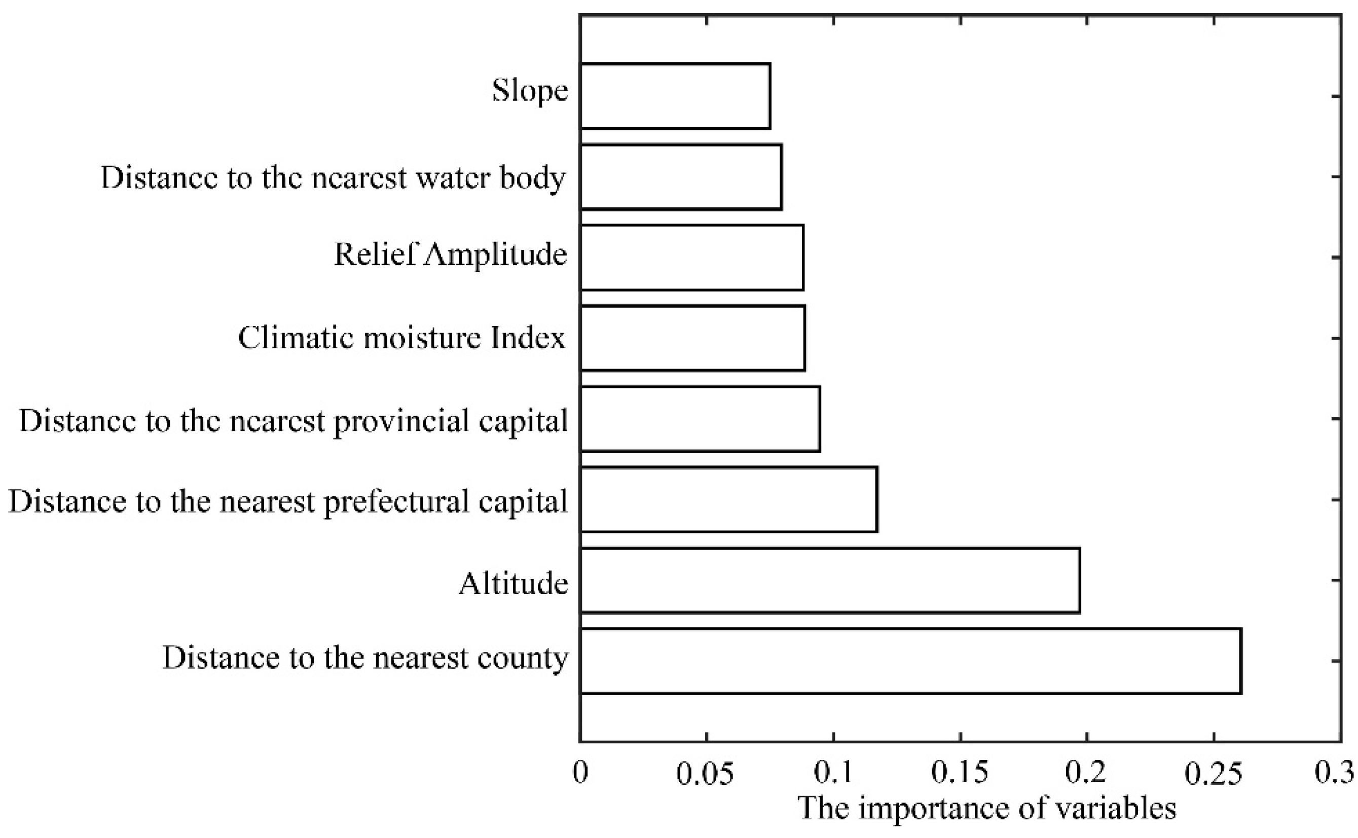
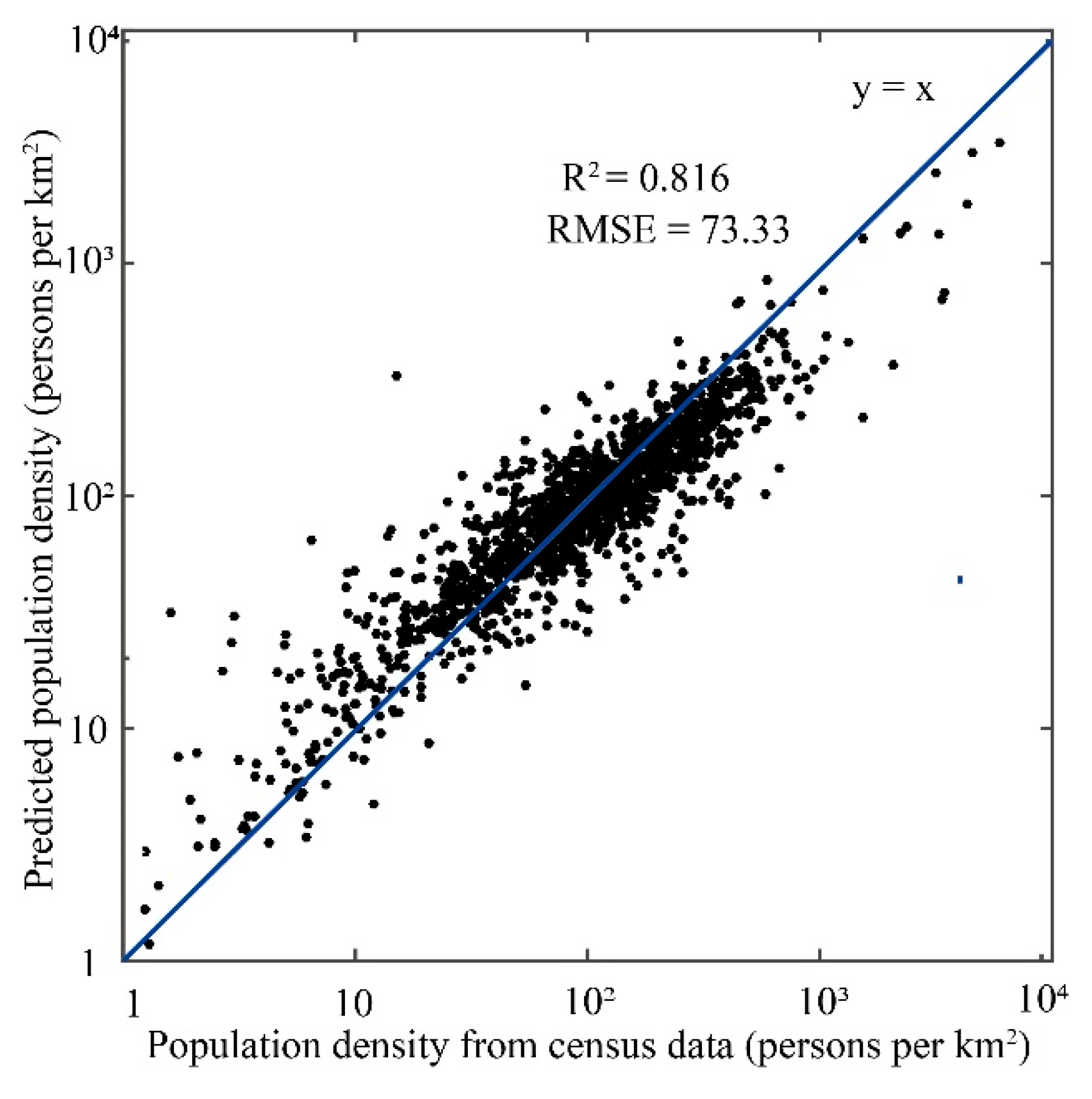
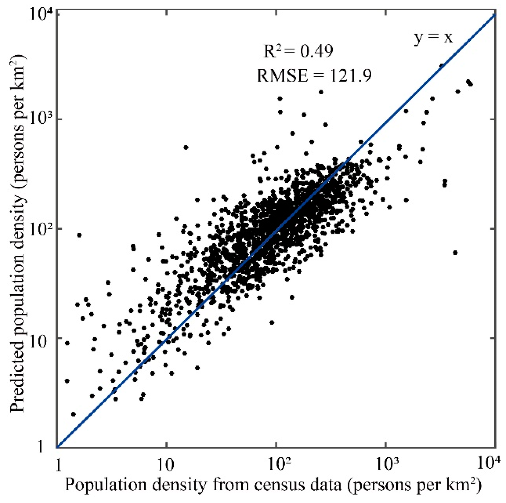
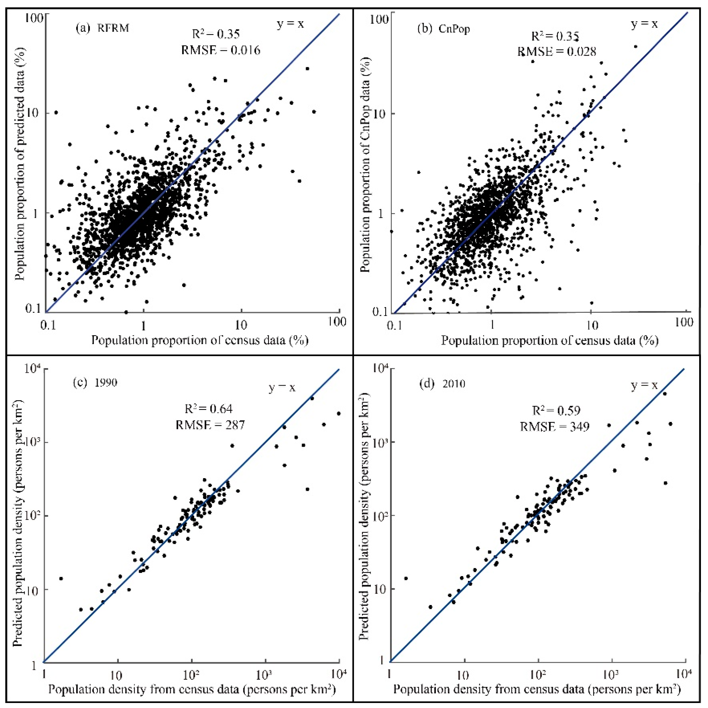
3.1. Evaluation of Model Performance

The RFRM predicted the natural logarithm of the population density. To highlight the performance of RFRM through comparing directly with the census data, the prediction with natural logarithm were converted to population density. Figure 5 shows that there was a significantly positive correlation (R² = 0.82) between the predicted population density and census data at the township level for 2000. This suggests that the RFRM driven by the abovementioned environmental factors was largely able to reproduce the spatial variability in the population distribution at the township level within Gansu Province. Nevertheless, it was found that errors exist and that the positive and negative errors always occurred in towns with low population density and high population density, respectively. Figure 6a confirms that the errors occur almost randomly and that the distributions of positive and negative errors were approximately symmetric with each other. In total, 81.58% of the towns had a relative error less than 50%, and only 8.55% of the towns had a relative error higher than 80%. Figure 6b shows that the positive and negative errors were evenly distributed in the large towns and small towns within Gansu Province, while the negative errors mainly occurred in the border towns of Gansu Province. Due to the complex natural and human factors of the border towns, the ability of the RFRM to predict the population density in those areas was weak. Another explanation may be the error of census data. Due to population mobility, the census coverage was usually higher in city and urban areas and lower in the rural areas, especially in the mountainous areas and remote districts. the actual population may be overestimated in the urban areas like cities and underestimated in the rural areas. Thus, the errors in those areas were relatively large. All of these findings, together with the positive reduction of error (RE = 0.72) and the coefficient of efficiency (CE = 0.65), suggest that the model is able to reproduce the spatial variability in population density and is likely stable.

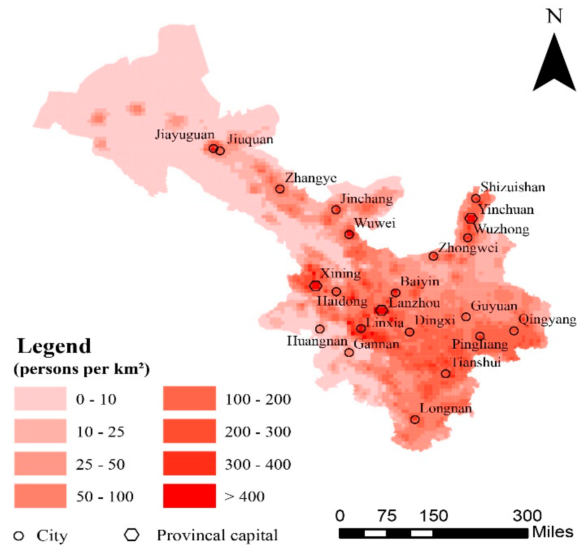
3.2. Modeling the Population Density in the 2000

Figure 7 shows the explicit population density variability in 10 by 10 km grid cells within the Gansu Province in 2000. We found that there was a high density of the population in the southeastern portion of Gansu Province and a low density of the population in the northwestern partition of the Tibetan Plateau. In central Gansu Province, the high population density mainly occurred in Lanzhou, Baiyin, Linxia, and Tianshui. The population density of the Lanzhou city reached 3986 persons per km². Due to the restriction of the Qilian Mountains, the population in the Hexi corridor was zonal distribution and exhibited an extension from southeast to the northwest. To the northeast, i.e., the Ningxia Plain, the high population density mainly occurred in the urban areas of cities and surrounding areas such as Yinchuan, Wuzhong, and Shizuishan. To the southwest, i.e., the northeastern portion of the Tibetan Plateau, the highest population density occurred in Xining city, with a population density of more than 1500 persons per km².

Furthermore, to evaluate the performance of RFRM in the 10- by 10-km grid cells, the RFRM predictions at the grid cell level were compared to the 2000 census at township level. The predictions in the grid cells were aggregated into data at the township scale to compare with the township level census. As shown in Figure 8, there are also significantly positive correlations, with determination coefficients of 0.49. It is possible that the RFRM grid cell-based predictions may perform well at predicting the spatial variability in population density within Gansu Province in 2000. However, there are errors, as shown by the root mean square error (RMSE) of 121.9 persons per km². The errors are likely random and have an approximately normal distribution. Both positive errors and negative errors exist, and moreover, there is a high frequency of small errors and low frequency of large errors. Positive errors mostly occurred in the areas with low population density, while negative errors mostly occurred in the areas with high population density. This finding suggests that grid cell-based RFRM predictions could not reproduce the areas of relatively low and high density of the population well.

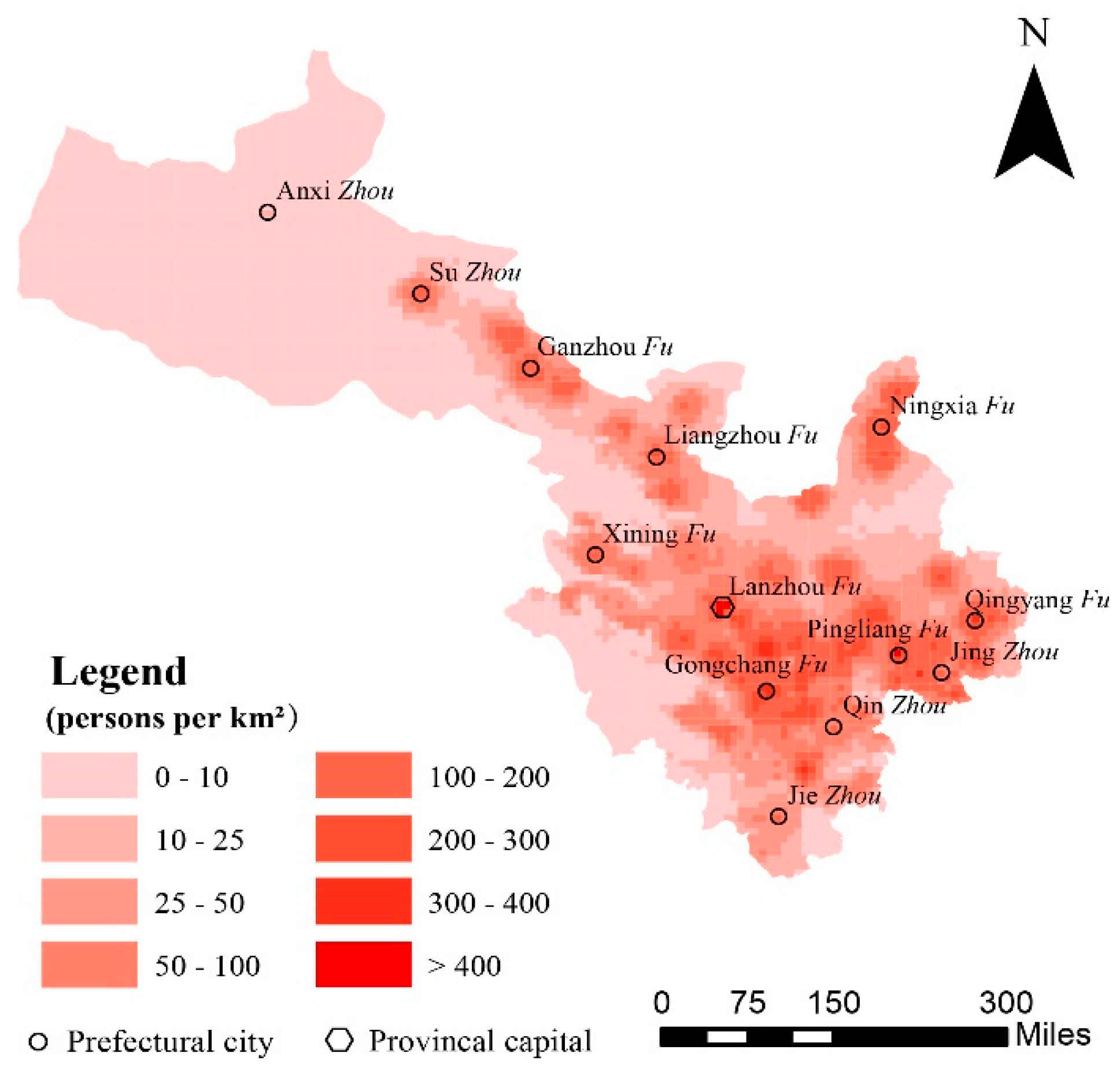
3.3. Modeling the Population Density in the 1820

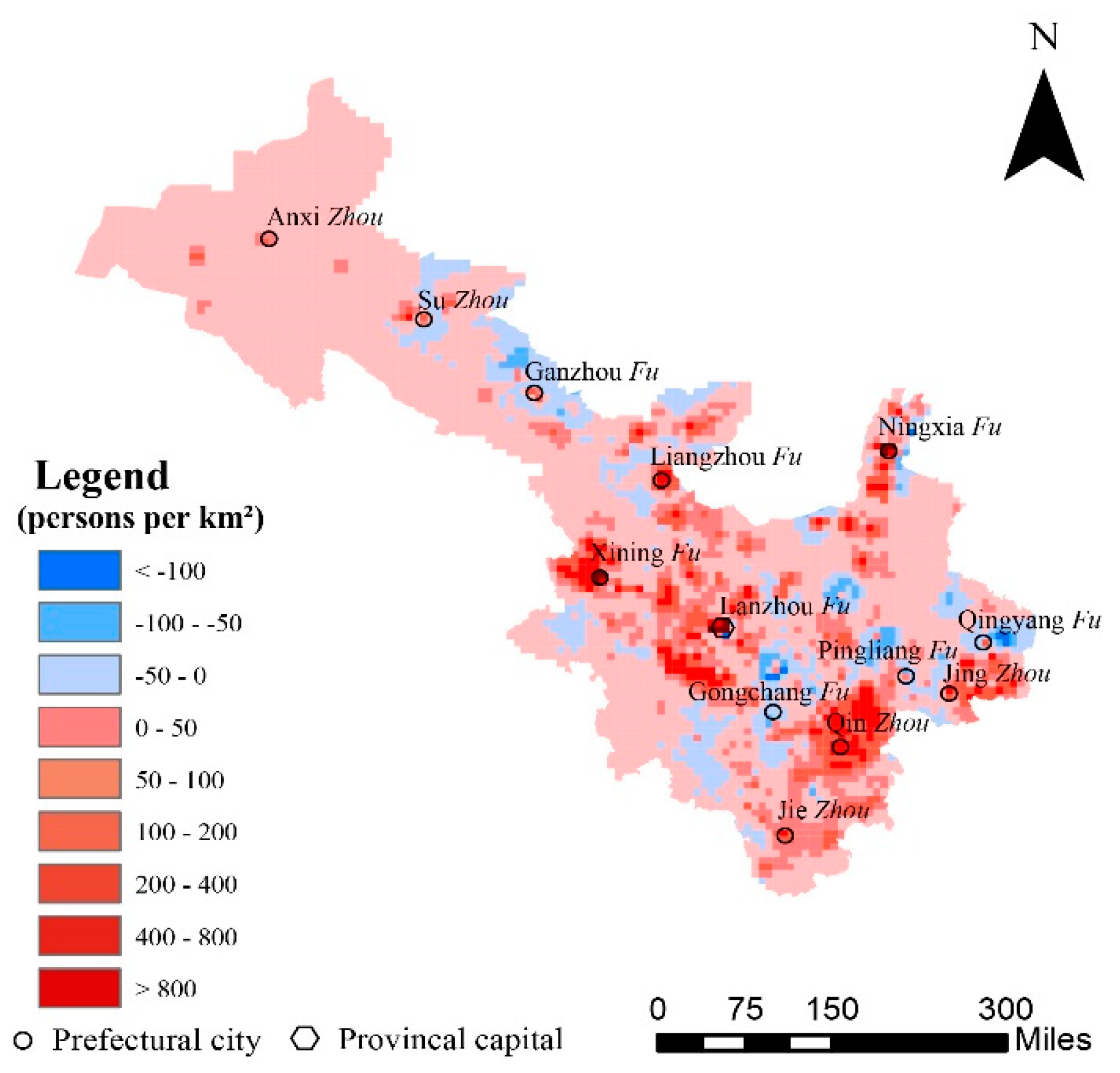
Figure 9 shows the RFRM grid cell-based predictions of population density with a spatial resolution of 10 by 10 km in Gansu Province in 1820. The overall spatial pattern of the population density in 1820 was approximately the same as that in 2000. There was a high population density in the southeastern region and a low population density in the northwestern region. However, the population density was quite different from that in 2000 in some regions. The population in 1820 was mostly distributed in the central and eastern portions of Gansu, the Ningxia Plain, the Hexi Corridor, and the northeastern Tibetan Plateau. In the central and eastern parts of Gansu, a higher population density existed mainly in Lanzhou, Gongchang, Pinglian, and Qingyang. For instance, in Lanzhou, the population density exceeded 1700 persons per km². In the Hexi Corridor, a high population density was mainly found in the Suzhou, Ganzhou, and Liangzhou city, with a population density of more than 100 persons per km². Moreover, the population in the Ningxia plain and northeastern Tibetan Plateau was densely distributed in Ningxia and Xining city, respectively. The population density in Ningxia reached more than 200 persons per km².

Figure 10 shows the differences in the population density of Gansu Province between 1820 and 2000. In comparison to 1820, the population in 2000 was denser in some areas while it was sparser in other areas. The intensified population density mainly occurred in Lanzhou, Xining, Ningxia, Qinzhou, and Jiezhou. With the increasing population aggregations in the provincial capital cities, the population in some grid cells of Lanzhou, Ningxia, and Xining city has increased by more than 800 persons per km². The weakened population density mainly occurred in Gongchang, Ganzhou, Suzhou, and Qinyang. The population density reductions in those areas can exceed 100 persons per km².

The demographic change in Gansu Province was primarily affected by the cities. Along with the urban development, the population aggregation effect in modern cities was strengthening. The cities especially the provincial capitals such as Lanzhou, Yinchuan, and Xining city had great attractiveness to the surrounding population, as the cites can provide more employment opportunities. The population was constantly floating from rural areas to the urban areas, thus the population was densely distributed in the urban areas of those cities. The dominant reason for the population decrease in some areas was the evolution of the structure of cities. The first reason for this may be the decline in a city’s political level. For instance, Gongchang was the capital of a prefectural unit, namely, Gongchang Fu in Chinese, in 1820. whereas, it was canceled and reset as a county in 1913. The second reason may be that a city was replaced by a new city. For instance, the capital of Heshui County, Qingyang Fu, in 1820 was replaced by the present-day capital. As a result, the population density around the old capital of Heshui County in 2000 was lower than that in 1820. The third reason for the population decrease may be related to military affairs. For instance, Ganzhou, and Suzhou were important military towns in the Northwest China in the historical period; however, the military positions are largely reduced at present. As a result, the population density in Ganzhou decreased from 41 persons per km² in 1820 to 31 persons per km² in 2000. In addition, affected by the climate and river change, the living condition in some extremely arid areas of Gansu Province became worse, it might have a certain impact on the population distribution.

To improve our understanding of the spatial variability in population density changes in Gansu Province, we analyzed the variations in the population density for areas with altitude above sea level.

Table 1. Variation in the population density with altitude above sea level.

Altitude (Meters)	Population in 1820 (104 Persons)	Population in 2000 (104 Persons)	Change (104 Persons)	Proportion of Population Growth (%)
<1500	520.11	906.74	386.63	23.60
1500–2000	684.54	1196.88	512.34	31.27
2000–2500	416.87	827.44	410.57	25.06
2500–3000	126.90	329.82	202.92	12.38
3000–3500	28.99	126.12	97.13	5.93
>3500	7.15	36.07	28.92	1.76
Total	1784.56	3423.06	1638.51	100

shows that most of the population existed in the lowlands, while less of the population existed in the highlands. The population in the area lower than 2500 m accounted for as much as 90.86% in 1820 and 85.63% in 2000. This finding illustrated that the vertical structure of the population distribution in Gansu Province was essentially stable from 1820 to 2000. However, the population growths varied with altitude. The total population in Gansu Province increased from 17.84 million in 1820 to 34.23 million in 2000, 79.92% of which occurred in the regions below 2500 m and only 7.69% of which occurred in the regions above 3000 m. The greatest increase occurred in areas between 1500 m and 2000 m. Moreover, the weighting of the highlands increased. The population in the area above 2500 m accounted for ~9% in 1820, and it increased to greater than 14% in 2000.

4. Discussion

In addition to the abovementioned comparisons between the RFRM predictions and census data, we also compared the RFRM predictions and the 1 by 1 km resolution China gridded population dataset (CnPop) to the township level census data for 2000, respectively. According to the previous studies, CnPop had a higher accuracy of estimation at the township level in China than of the other gridded population datasets, e.g., GPW and WorldPop [51]. Since the RFRM prediction and CnPop dataset are based on grid cells and the census data were collected at the township level, we aggregated the grid cell-based RFRM prediction and CnPop dataset into townships. Additionally, because the census data sources were different from the data source used by the CnPop dataset, the population proportion of each town to the prefectural unit was calculated and compared with each other.

Figure 11a,b show that both the RFRM prediction and CnPop dataset perform well at reproducing the spatial variability in the weighted township-level population within the prefectural unit, with a determination coefficient of 0.35. Moreover, both the CnPop dataset and RFRM prediction exhibit random errors. However, the RMSE of RFRM predictions (0.016) is slightly lower than the RMSE of CnPop dataset (0.028). Taken together, these findings indicate that RFRM predictions use fewer environmental variables than the CnPop dataset does, RFRM grid cell-based predictions accurately reproduced the spatial variability in population density, and the performance of RFRM is comparable to the existing CnPop dataset. In addition, the population distribution of Gansu Province in 1990 and 2010 were reproduced at the gird scale, then they were aggregated into county and compared with the census data. Figure 11c,d show that the RFRM has a good prediction accuracy with the determination coefficients of about 0.6. The RFRM approach is, hence, suitable for historical periods.

It is noted that some uncertainties exist in this study. Firstly, as mentioned above, the historical population distribution was influenced by the political situation and climate change, those factors can’t be quantified in the RFRM, so the RFRM can’t express the impacts of those factors on population distribution. Secondly, the environmental factors of 2000 used in 1820 may be not suitable. For example, climate moisture was used as an environmental factor. Due to the lack of precise environmental moisture data for 1820, the present moisture spatial pattern of moisture was used in this study. However, the climate proxy data shows that there may have been significant climate changes from 1820, which was in the period of the Little Ice Age, to 2000 [52]. Additionally, this study used the quantitative relations between the population density and distance to the nearest city derived from data for 2000 in the 1820 reconstruction. In 2000, this region had an industrial and commercial society, whereas, it had an agricultural society in 1820. Because the livelihoods are different, the importance of the city is also different. As a result, the quantitative relations between the population density and distance to the nearest city derived from data for 2000 would not be completely suitable for 1820. Finally, the census data in 1820 may suffer from a distinct bias compared with it in 2000, which mainly caused by the different statistical criteria between historical and contemporary census, it might lead to errors of population comparison in some areas.

5. Conclusions

This paper presents an RFRM-based population gridding method that is able to reproduce the explicit distribution of populations in historical periods. Using the RFRM, we constructed the explicit population distributions of Gansu Province in 1820 and 2000 for 10- by 10-km grid cells. The results suggest that the RFRM together with the available environmental factors, fits the census data well. The spatial pattern of the population density of Gansu Province in 2000 kept approximately similar with that in 1820; however, explicit differences exist. In comparison to 1820, the population density in 2000 intensified in many cities, such as Lanzhou, Xining, Yinchuan, Baiyin, Linxia, and Tianshui, while it weakened in other cities, such as Gongchang, Qingyang, Ganzhou, and Suzhou. The decreased population may be mainly caused by the decline in cities’ political and military positions. Moreover, we also found that 79.92% of the population increase from 1820 to 2000 occurred in areas lower than 2500 m. However, due to relatively high increasing rate, the population weighting of areas above 2500 m increased from ~9% in 1820 to greater than 14% in 2000.

This study presents the spatial variability in the population density changes in Gansu Province from 1820 to 2000. More importantly, it provides the community a dataset for the spatially explicit population density of Gansu Province in 1820 and 2000. This dataset will be valuable for population-relevant issues and studies. We found that the RFRM predictions do incur errors, which are comparable to the error of the existing CnPop dataset. However, the RFRM predictions relied on a few environmental factors, which is much less than required by the CnPop dataset, and RFRM is, therefore, better suitable for historical spatially explicit reconstruction of the population.

References

1. Fuguitt, G.V.; Zuiches, J.J. Residential Preferences and Population Distribution. Demography 1975, 12, 491. [Google Scholar] [CrossRef] [PubMed]
2. Yue, T.X.; Wang, Y.A.; Liu, J.Y.; Chen, S.P.; Qiu, D.S.; Deng, X.Z.; Liu, M.L.; Tian, Y.Z.; Su, B.P. Surface modelling of human population distribution in China. Ecol. Model. 2005, 181, 461–478. [Google Scholar] [CrossRef]
3. Balk, D.L.; Deichmann, U.; Yetman, G.; Pozzi, F.; Hay, S.I.; Nelson, A. Determining global population distribution: Methods, applications and data. Adv. Parasitol. 2006, 62, 119–156. [Google Scholar] [PubMed] [Green Version]
4. Tobler, W.; Deichmann, U.; Gottsegen, J.; Maloy, K. World population in a grid of spherical quadrilaterals. Int. J. Popul. Geogr. 1997, 3, 203–225. [Google Scholar] [CrossRef]
5. Wu, J.; Mohamed, R.; Wang, Z. Agent-based simulation of the spatial evolution of the historical population in China. J. Hist. Geogr. 2011, 37, 12–21. [Google Scholar] [CrossRef]
6. Klein Goldewijk, K.; Beusen, A.; Van Drecht, G.; De Vos, M. The HYDE 3.1 spatially explicit database of human-induced global land-use change over the past 12,000 years. Glob. Ecol. Biogeogr. 2011, 20, 73–86. [Google Scholar] [CrossRef]
7. Lin, S.; Zheng, J.; He, F. Gridding cropland data reconstruction over the agricultural region of China in 1820. J. Geogr. Sci. 2009, 19, 36–48. [Google Scholar] [CrossRef]
8. Arneth, A.; Sitch, S.; Pongratz, J.; Stocker, B.D.; Ciais, P.; Poulter, B.; Bayer, A.D.; Bondeau, A.; Calle, L.; Calle, L.; et al. Historical carbon dioxide emissions caused by land-use changes are possibly larger than assumed. Nat. Geosci. 2017, 10, 79. [Google Scholar] [CrossRef]
9. Leyk, S.; Gaughan, A.E.; Adamo, S.B.; de Sherbinin, A.; Balk, D.; Freire, S.; Rose, A.; Stevens, F.R.; Blankespoor, B.; Frye, C.; et al. The spatial allocation of population: A review of large-scale gridded population data products and their fitness for use. Earth Syst. Sci. Data 2019, 11, 1385–1409. [Google Scholar] [CrossRef] [Green Version]
10. Islam, M.S.; Oki, T.; Kanae, S.; Hanasaki, N.; Agata, Y.; Yoshimura, K. A grid-based assessment of global water scarcity including virtual water trading. Water Resour. Manag. 2007, 21, 19. [Google Scholar] [CrossRef]
11. Dasgupta, S.; Laplante, B.; Murray, S.; Wheeler, D. Exposure of developing countries to sea-level rise and storm surges. Clim. Chang. 2011, 106, 567–579. [Google Scholar] [CrossRef]
12. Mondal, P.; Tatem, A.J. Uncertainties in Measuring Populations Potentially Impacted by Sea Level Rise and Coastal Flooding. PLoS ONE 2012, 7, e48191. [Google Scholar] [CrossRef] [PubMed]
13. Hay, S.I.; Noor, A.M.; Nelson, A.; Tatem, A.J. The accuracy of human population maps for public health application. Trop. Med. Int. Health 2005, 10, 1073–1086. [Google Scholar] [CrossRef]
14. Lam, N.S.N. Spatial interpolation methods: A review. Am. Cartogr. 1983, 10, 129–150. [Google Scholar] [CrossRef]
15. De Amorim Borges, P.; Franke, J.; da Anunciação, Y.M.T.; Weiss, H.; Bernhofer, C. Comparison of spatial interpolation methods for the estimation of precipitation distribution in Distrito Federal, Brazil. Theor. Appl. Climatol. 2016, 123, 335–348. [Google Scholar] [CrossRef]
16. Azar, D.; Engstrom, R.; Graesser, J.; Comenetz, J. Generation of fine-scale population layers using multi-resolution satellite imagery and geospatial data. Remote Sens. Environ. 2013, 130, 219–232. [Google Scholar] [CrossRef]
17. Zeng, C.; Zhou, Y.; Wang, S.; Yan, F.; Zhao, Q. Population spatialization in China based on night-time imagery and land use data. Int. J. Remote Sens. 2011, 32, 9599–9620. [Google Scholar] [CrossRef]
18. Hu, L.; He, Z.; Liu, J. Adaptive Multi-Scale Population Spatialization Model Constrained by Multiple Factors: A Case Study of Russia. Cartogr. J. 2011, 54, 265–282. [Google Scholar] [CrossRef]
19. Zhuo, L.; Ichinose, T.; Zheng, J.; Chen, J.; Shi, P.J.; Li, X. Modelling the population density of China at the pixel level based on DMSP/OLS non-radiance-calibrated night-time light images. Int. J. Remote Sens. 2009, 30, 1003–1018. [Google Scholar] [CrossRef]
20. Tan, M.; Li, X.; Li, S.; Xin, L.; Wang, X.; Li, Q.; Li, W.; Li, Y.; Xiang, W. Modeling population density based on nighttime light images and land use data in China. Appl. Geogr. 2018, 90, 239–247. [Google Scholar] [CrossRef]
21. Calka, B.; Nowak Da Costa, J.; Bielecka, E. Fine scale population density data and its application in risk assessment. Geomatics. Nat. Hazards Risk 2017, 8, 1440–1455. [Google Scholar] [CrossRef]
22. Stevens, F.R.; Gaughan, A.E.; Linard, C.; Tatem, A.J. Disaggregating census data for population mapping using random forests with remotely-sensed and ancillary data. PLoS ONE 2015, 10, e0107042. [Google Scholar] [CrossRef] [PubMed] [Green Version]
23. Youssef, A.M.; Pourghasemi, H.R.; Pourtaghi, Z.S.; Al-Katheeri, M.M. Landslide susceptibility mapping using random forest, boosted regression tree, classification and regression tree, and general linear models and comparison of their performance at Wadi Tayyah Basin, Asir Region, Saudi Arabia. Landslides 2016, 13, 839–856. [Google Scholar] [CrossRef]
24. Zhang, H.; Wu, P.; Yin, A.; Yang, X.; Zhang, M.; Gao, C. Prediction of soil organic carbon in an intensively managed reclamation zone of eastern China: A comparison of multiple linear regressions and the random forest model. Sci. Total Environ. 2017, 592, 704–713. [Google Scholar] [CrossRef]
25. Forkuor, G.; Hounkpatin, O.K.; Welp, G.; Thiel, M. High resolution mapping of soil properties using remote sensing variables in south-western Burkina Faso: A comparison of machine learning and multiple linear regression models. PLoS ONE 2017, 12, e0170478. [Google Scholar] [CrossRef]
26. Ye, T.; Zhao, N.; Yang, X.; Ouyang, Z.; Liu, X.; Chen, Q.; Hu, K.; Yue, W.; Qi, J.; Li, Z.; et al. Improved population mapping for China using remotely sensed and points-of-interest data within a random forests model. Sci. Total Environ. 2019, 658, 936–946. [Google Scholar] [CrossRef]
27. Li, H.; Liu, F.; Cui, Y.; Ren, L.; Storozum, M.J.; Qin, Z.; Wang, J.; Dong, G. Human settlement and its influencing factors during the historical period in an oasis-desert transition zone of Dunhuang, Hexi Corridor, northwest China. Quat. Int. 2017, 458, 113–122. [Google Scholar] [CrossRef]
28. Zinyama, L.; Whitlow, R. Changing patterns of population distribution in Zimbabwe. GeoJournal 1986, 13, 365–384. [Google Scholar] [CrossRef]
29. Wang, P.; Wang, Z.W.; Zhang, X.T.; Wang, X.; Feng, Q.S.; Chen, Q.G. The Spatial Patterns of China’s Population and Their Cause of Format ion in Western Han Dynasty. Northwest Popul. J. 2010, 5, 88–90. [Google Scholar]
30. Dong, G.; Yang, Y.; Zhao, Y.; Zhou, A.; Zhang, X.; Li, X.; Chen, F. Human settlement and human-environment interactions during the historical period in Zhuanglang County, western Loess Plateau, China. Quat. Int. 2012, 281, 78–83. [Google Scholar] [CrossRef]
31. Small, C.; Cohen, J. Continental physiography, climate, and the global distribution of human population. Curr. Anthropol. 2004, 45, 269–277. [Google Scholar] [CrossRef]
32. Kummu, M.; De Moel, H.; Salvucci, G.; Viviroli, D.; Ward, P.J.; Varis, O. Over the hills and further away from coast: Global geospatial patterns of human and environment over the 20th–21st centuries. Environ. Res. Lett. 2016, 11, 034010. [Google Scholar] [CrossRef]
33. Cohen, J.E.; Small, C. Hypsographic demography: The distribution of human population by altitude. Proc. Natl. Acad. Sci. USA 1998, 95, 14009–14014. [Google Scholar] [CrossRef] [PubMed] [Green Version]
34. Feng, Z.; Tang, Y.; Yang, Y.; Zhang, D. Relief degree of land surface and its influence on population distribution in China. J. Geogr. Sci. 2008, 18, 237–246. [Google Scholar] [CrossRef]
35. Dong, N.; Yang, X.; Cai, H. Research progress and perspective on the spatialization of population data. J. Geo-Inf. Sci. 2016, 18, 1295–1304. [Google Scholar]
36. Liu, Y.; Deng, W.; Song, X. Relief degree of land surface and population distribution of mountainous areas in China. J. Mt. Sci. 2015, 12, 518–532. [Google Scholar] [CrossRef]
37. Xu, X.; Zhang, Y. Chinese meteorological background dataset. Resources and Environmental Scientific Data Center (RESDC). Chin. Acad. Sci. CAS 2017. [Google Scholar] [CrossRef]
38. Cao, S.J. Population History of China (Vol. 5, Qing Dynasty Period); Fudan University Press: Shanghai, China, 2007; pp. 690–720. [Google Scholar]
39. Lu, W.D. Fifty Years of Population in Northwest China (1861–1911); Fudan University Press: Shanghai, China, 2017; pp. 135–136. [Google Scholar]
40. Department of Population Social Science and Technology Statistics National Bureau of Statistics of China. China Population by Township; China Statistics Press: Beijing, China, 2002.
41. Breiman, L. Random forests. Mach. Learn. 2001, 45, 5–32. [Google Scholar] [CrossRef] [Green Version]
42. Biau, G. Analysis of a random forests model. J. Mach. Learn. Res. 2012, 13, 1063–1095. [Google Scholar]
43. Rodriguez-Galiano, V.; Mendes, M.P.; Garcia-Soldado, M.J.; Chica-Olmo, M.; Ribeiro, L. Predictive modeling of groundwater nitrate pollution using Random Forest and multisource variables related to intrinsic and specific vulnerability: A case study in an agricultural setting (Southern Spain). Sci. Total Environ. 2014, 476, 189–206. [Google Scholar] [CrossRef]
44. Liaw, A.; Wiener, M. Classification and regression by randomForest. R News 2002, 2, 18–22. [Google Scholar]
45. Strobl, C.; Boulesteix, A.L.; Kneib, T.; Augustin, T.; Zeileis, A. Conditional variable importance for random forests. BMC Bioinform. 2008, 9, 307. [Google Scholar] [CrossRef] [PubMed] [Green Version]
46. Wang, L.A.; Zhou, X.; Zhu, X.; Dong, Z.; Guo, W. Estimation of biomass in wheat using random forest regression algorithm and remote sensing data. Crop J. 2016, 4, 212–219. [Google Scholar] [CrossRef] [Green Version]
47. Li, K.; Chen, Y.; Li, Y. The Random Forest-Based Method of Fine-Resolution Population Spatialization by Using the International Space Station Nighttime Photography and Social Sensing Data. Remote Sens. 2018, 10, 1650. [Google Scholar] [CrossRef] [Green Version]
48. Tan, M.; Liu, K.; Lin, L.; Zhu, Y.; Wang, D. Spatialization of population in the Pearl River Delta in 30 m grids using random forest model. Prog. Geogr. 2017, 36, 1304–1312. [Google Scholar]
49. Michaelsen, J. Cross-validation in statistical climate forecast models. J. Clim. Appl. Meteorol. 1987, 26, 1589–1600. [Google Scholar] [CrossRef] [Green Version]
50. Gou, X.; Gao, L.; Deng, Y.; Chen, F.; Yang, M.; Still, C. An 850-year tree-ring-based reconstruction of drought history in the western Qilian Mountains of northwestern China. Int. J. Climatol. 2015, 35, 3308–3319. [Google Scholar] [CrossRef]
51. Bai, Z.; Wang, J.; Wang, M.; Gao, M.; Sun, J. Accuracy assessment of multi-source gridded population distribution datasets in China. Sustainability 2018, 10, 1363. [Google Scholar] [CrossRef] [Green Version]
52. Gou, X.; Deng, Y.; Gao, L.; Chen, F.; Cook, E.; Yang, M.; Zhang, F. Millennium tree-ring reconstruction of drought variability in the eastern Qilian Mountains, northwest China. Clim. Dyn. 2015, 45, 1761–1770. [Google Scholar] [CrossRef] [Green Version]
Figure 1. Map of Gansu Province in year 1820 (the bottom-left insert shows the location of the study area in China).
Sustainability 12 01231 g001
Figure 2. Histogram of environmental factors distribution.
Sustainability 12 01231 g002
Figure 3. Importance of variables in random forest regression model (RFRM).
Sustainability 12 01231 g003
Figure 4. The dependence of RFRM accuracy on the max_features under different n_estimators.
Sustainability 12 01231 g004
Figure 5. The RFRM predictions with the leave-one-out method plotted against the 2000 Census data at the township level. Abbreviations: RMSE, root mean square error.
Sustainability 12 01231 g005
Figure 6. Histogram (a) and spatial distributions (b) of relative errors of the RFRM predictions with the leave-one-out method at the township level for the 2000.
Sustainability 12 01231 g006
Figure 7. Population density in 2000 in 10- by 10-km grid cells.
Sustainability 12 01231 g007
Figure 8. Comparison of the RFRM grid cell-based predictions aggregated into township with the township level census data for 2000.
Sustainability 12 01231 g008
Figure 9. Population density of Gansu Province in 1820 in 10- by 10-km grid cells.
Sustainability 12 01231 g009
Figure 10. Population density differences in Gansu Province between 1820 and 2000 at cell size of 10 by 10 km.
Sustainability 12 01231 g010
Figure 11. Population proportion of the townships to the prefectures from the RFRM grid cell-based predictions (a) and from the China 1 km Gridded Population (CnPop) dataset (b) plotted against that from the census and comparison of the RFRM grid cell-based predictions aggregated into county with the county level census data for 1990 (c) and 2010 (d), respectively.
Sustainability 12 01231 g011