Investigating the Ripple Effect through the Relationship between Housing Markets and Residential Migration in Seoul, South Korea

Abstract

This study examined the relationship between housing markets and residential migration to identify if there is a housing refugee phenomenon due to an involuntary ripple effect in the Seoul metropolitan area, South Korea. The study applied Granger causality analysis and a vector error correction model. The empirical results confirmed that changes in housing market conditions cause a ripple effect in surrounding areas in the Seoul metropolitan area, and these changes are easily transmitted to the nearby Gyeonggi housing market. This study shows that intra-metropolitan residential migration may occur due to changes in housing market conditions. Additionally, the study proved that residential migration from Seoul to the nearby Gyeonggi province does not represent the pursuit of a stable residential environment, but is merely involuntary migration due to the financial burden of increased housing costs in Seoul. Finally, the study showed that there may be a ripple effect that intensifies instability in the jeonse market—a type of lease unique to South Korea—that emerged due to residential migration from Seoul. From this perspective, this study confirms that residential migration occurring in the Seoul metropolitan area is the result of an involuntary ripple effect and represents a housing refugee phenomenon.

1. Introduction

The housing market in South Korea is experiencing substantial change due to the economic downturn. The most remarkable change is that a housing price trend that rapidly gathered stream in the 2000s has subsided, thereby reducing the possibility of capital gains from profit margins on purchases and sales. This change has shifted the direction of the South Korean housing market. Property owners are seeking operating profit in the form of rent rather than gains on sales. Moreover, the demand for housing purchases has decreased while the demand for leasing has increased. Particularly, the market for jeonse, a type of housing lease unique to South Korea, is falling into a state of chaos. With a jeonse arrangement, the lessee can pay a certain amount of deposit (approximately 40% to 70% of the sales price) in a lump sum without having to pay monthly rent to live in the housing [1,2,3,4]. It was the case that a lessor would rent their property by receiving the jeonse deposit of approximately 70% of the sales price, which the lessor would bank to receive interest or use in other investments. However, as the usability of the jeonse deposit has decreased due to slow economic growth and low interest rates, the trend is shifting towards monthly rent (wolse in Korean), whereby the lessor can realize a higher profit than they would through bank interest.

According to data released by the South Korean Ministry of Land, Infrastructure, and Transport, the percentage of apartment—a type of housing that is common and preferred in South Korea—monthly rent from lease/rental contracts nationwide increased from 24.6% in 2011 to 40.5% in mid-2016 and from 17.4% to 38.3% in Seoul. The ratio of monthly rent in Seoul more than doubled in five years. On the other hand, tenants who cannot afford to purchase housing prefer jeonse over monthly rents because they pay a deposit of approximately 70% of the sales price and receive all their deposit back when the lease ends. Accordingly, the demand for jeonse is increasing while the supply is decreasing causing a market imbalance. As jeonse prices constantly increase due to the mismatch between supply and demand, the required deposit amounts have increased to unaffordable levels of up to 90% of the sales price in some parts of Seoul. This phenomenon is more apparent in the housing market in Seoul, the capital and economic center of South Korea, where housing prices are highest. Jeonse households in Seoul are forced to extend their lease by obtaining a loan to pay the increased deposits or by moving to less expensive nearby areas such as Gyeonggi province. The upward trend in sales prices has also halted; however, the price-to-income ratio (PIR) is 11.2, which is higher than that in Los Angeles, London, New York, and Tokyo, indicating that it is much more difficult to purchase a house in Seoul [5].

If the increase in jeonse prices and high sales prices in Seoul force residents to move to Gyeonggi province, which is next to Seoul, there will be a chain reaction and a significant impact on the housing market in Gyeonggi province [6,7]. According to Trends in National Housing Prices surveyed by the South Korea Appraisal Board, the average annual increase in nationwide jeonse prices from 2013 to 2017 was 2.98%, whereas it was 4.3% in the metropolitan area including Seoul and Gyeonggi province. These data indicate that acquiring jeonse residency is more difficult in this area compared to other regions. The average housing price in Seoul, as of 2017, was KRW 660 million (approximately USD 580,000), which is more than twice the price of housing in Gyeonggi province (KRW 320 million, USD 280,000) further aggravating the conditions for property ownership in Seoul. Net migration to Gyeonggi province from Seoul is also constantly increasing and, since 2015, the population moving from Seoul to Gyeonggi province has rapidly increased by at least 26%. According to the population migration data by Statistics Korea, net migration from Seoul to Gyeonggi province from July 2010 to February 2015 was 8017 a year, on average, but it rapidly increased by at least 26.4% to 10,134 from March 2015 to August 2017. Residential migration reflects the housing market conditions in Seoul, which suggests a strong relationship between the housing market and residential migration.

Although a ripple effect on the metropolitan housing market is expected following changes in housing market conditions in Seoul, the nation’s capital, there has been insufficient microscopic analysis on whether there is actually a ripple effect on the housing markets of Seoul and Gyeonggi province and the interactions occurring in the housing market. The main reason for investigating the ripple effect in a metropolitan area is because residential migration is likely to cause various problems related to housing stability in metropolitan areas, which could trigger further instability in the housing market. Thus, the purpose of this study is to examine the changes in metropolitan area housing market conditions and their relationship with residential migration. This study empirically analyzes whether there is a ripple effect using Granger causality analysis and a vector autoregressive (VAR) model. Specifically, this study verifies whether changes in the sales and jeonse prices of the Seoul housing market cause residential migration to Gyeonggi province and whether residential migration brings changes to the housing market in the metropolitan area. Additionally, this study reviews whether residential migration in the metropolitan area is a ripple effect of involuntary migration—a housing refugee phenomenon.

The rest of this paper is organized as follows. Section 2 reviews the research background. Section 3 presents the current housing market and residential migration trends in the Seoul metropolitan area. Section 4 discusses the methodology and variable specification, and Section 5 presents the descriptive statistics and unit root test. Section 6 provides the empirical results of the Granger causality analysis, VAR, and impulse response analysis and forecast error variance decomposition analysis. Finally, Section 7 presents the conclusions and findings.

2. Research Background

Studies on the spatial transition phenomenon, whereby changes in housing prices in one region affect housing markets in nearby regions, have been conducted in various countries such as the United Kingdom [6,8,9,10,11,12,13,14], Australia [15,16], New Zealand [17], the United States [18], China [19,20,21], and South Korea [4,22,23,24,25,26].

The price transition phenomenon among housing markets is explained by the ripple effect, which has been actively discussed since Munro and McLennan [27]. The emergence of the phenomenon has raised the need for interregional correlation analysis of housing prices. A ripple effect is defined as a situation in which changes in a specific country or region’s housing prices directly affect another country or region’s housing market [6,10,11,13,19]. Housing markets integrate both the concepts of dependency and independency. Under the concept of dependency, the housing market has multiple hierarchical levels, and higher-level housing markets form a subordinate relationship with lower-level housing markets [13]. As a higher-level housing market assumes control as the price leader over the lower-level housing market, there is a ripple effect [28]. However, the housing market under the concept of independency is structurally differentiated from other housing markets with its own unique economic situation and demographic characteristics and is not influenced by others [13,17].

Some studies argued that the ripple effect does not appear among housing markets [8,15]. Nevertheless, many studies have found a ripple effect among housing markets. For example, Jones and Leishman [6] and Giussani and Hadjimatheou [11] examined whether there is a ripple effect in the local housing markets in the United Kingdom and concluded that there is a ripple effect on regions that are near other regions with high population density and large economic size. Meen [13] and Shi et al. [17] also conducted an analysis on the same country and verified a ripple effect among regions. Macdonald [29] and Cook [30] conducted an empirical analysis and determined that although there is a ripple effect in the UK housing market, there is a difference in the transition speed among regions.

Pollakowski and Ray [18] analyzed the ripple effect of changes in the housing market conditions of New York on its surrounding areas and proved that price changes in the New York housing market forms causality with nearby regions. However, the ripple effect is limited to regions next to metropolitan areas.

Chiang [19] examined the interregional transition of housing prices on six cities in China using a causality test and concluded that there is a clear interregional ripple effect. This study emphasized that Beijing housing prices represent a key driving force that increases the housing prices in surrounding regions. Therefore, it is necessary to develop a selective price policy targeting Beijing to stabilize housing prices. Huang et al. [20] examined the ripple effect of housing prices in 19 cities in China and verified that there was a ripple effect around metropolitan areas. Zhang et al. [21] stated that the ripple effect is not a local phenomenon limited to certain areas and proved that this pattern is evident in most Chinese cities.

However, contrary to this argument, Lee and Chien [31] found that the ripple effect appears only in small and medium cities and not metropolitan areas. Specifically, the authors analyzed five cities in Taiwan and discovered that there was a long-run relationship in cities except for the city of Taipei. This study clarified that the interregional ripple effect according to changes in housing prices may be a general phenomenon, but not all regions show the same pattern.

Related studies have also been conducted in South Korea, which is the target area of this study. Choi et al. [23] examined seven major cities including south and north Seoul and found a spillover effect in housing prices. The results showed that price changes in south Seoul, which has the highest housing prices in South Korea, affect not only north Seoul but also six other major cities located far away. Lee and Lee [26] also determined an interregional transition effect using apartment sales prices in the same region and arrived at the same conclusion. Chang [32] and Kim [33] empirically analyzed whether changes in housing prices in Seoul caused a ripple effect in the housing markets of other regions and discovered a ripple effect in areas near Seoul. However, unlike previous studies, they discovered that most regions that are geographically distant had little or no effect.

There are other studies that determined a ripple effect by including the jeonse housing market. Kim et al. [4] classified the South Korean housing market into a housing transaction market, a jeonse market, and a monthly rental market and examined their dynamic relations. The results showed that the global financial crisis in the late 2000s affected the South Korean economy. Lessors began to prefer monthly rent over jeonse, and this preference resulted in a rise in jeonse prices due to a supply–demand imbalance. In this situation, jeonse tenants could neither purchase housing due to a lack of liquidity nor easily pay the increased jeonse deposit, which pushed them involuntarily into the monthly rental market. Jin and Lee [25] analyzed the spatio-temporal interaction pattern of housing sales and jeonse prices in the Seoul metropolitan area using the SpVAR model. The authors proved that sales prices did not show a ripple effect on nearby areas, but jeonse prices were being transmitted to jeonse prices of surrounding areas. A few studies adopted a more microscopic approach and determined whether housing price changes in Gangnam, Seoul, where the housing prices are the highest in South Korea, cause a ripple effect on nearby areas. Those studies concluded that both sales prices and jeonse prices show an interregional spillover effect [22,24].

Many studies have proven that there is a ripple effect among housing markets in many countries, including South Korea. These ripple effects may have disturbed the stability of the housing markets. Changes in the social and economic conditions of Seoul significantly influence the housing markets nearby. This may exacerbate the confusion in the subordinate housing market as described. In particular, the ripple effect of the jeonse market appeared to be significant, thereby increasing pressure on jeonse tenants who did not accumulate much wealth [25]. However, previous studies focused on the spatial transition of housing prices while being limited in microscopically examining the changes among housing markets caused by the ripple effect. Interregional transition due to changes in sales and jeonse prices of certain regions appears in line with residential migration, which may become a factor that increases instability in the housing markets. Thus, this study considers it necessary to review the relationship between residential migration and changes in housing market conditions to understand the national and regional housing markets. Accordingly, this study overcomes the limitations of previous studies by reviewing how the changes in housing market conditions in Seoul and residential migration are causing a ripple effect on the surrounding housing markets. This study microscopically reviewed whether residential migration from Seoul to nearby Gyeonggi province is involuntary by specifically determining the ripple effect of the sales market and the jeonse market that is unique to South Korea. This study also examined whether the findings could represent a housing refugee phenomenon in the Seoul metropolitan housing market.

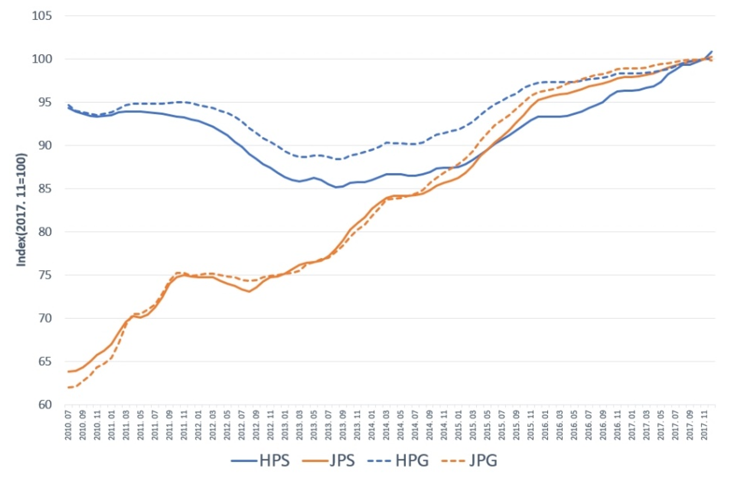
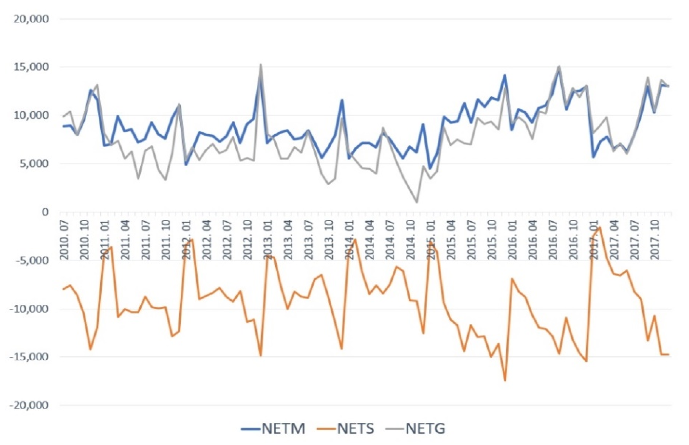
3. Housing Market and Residential Migration Trends in the Seoul Metropolitan Area

South Korea is currently in a state of flux due to the decoupling of the sales and jeonse markets. Typically, jeonse prices increase along with sales prices, building a positive correlation between the two. However, the expected gain from profit margins on purchases and sales recently decreased, which led to an increase in the demand for jeonse. Meanwhile, low interest rates and the economic recession lowered the usability of deposits and reduced jeonse supply, thereby increasing jeonse prices and causing a decoupling of the housing markets [4]. Decoupling is evident in the Seoul metropolitan area, where half the South Korean population is concentrated. Jeonse prices have increased at a rapid rate since the 2010s, but the rate of increase in sales prices is relatively lower than the increase in jeonse prices. Moreover, sales prices or jeonse prices in Gyeonggi province follow those in Seoul. Thus, Seoul recorded a higher rate of increase in sales prices than Gyeonggi province until the early 2010s, but Gyeonggi province showed a higher rate of increase after that. For jeonse, Gyeonggi province has shown a higher rate of increase in jeonse prices than Seoul since the early 2010s, which indicates that the housing market in Gyeonggi province changed significantly. Furthermore, Seoul and Gyeonggi province both showed a much higher increase in jeonse prices than sales prices (see Figure 1).

This study examined this trend using the transaction volume of housing (apartments) in the metropolitan area. According to the Ministry of Land, Infrastructure and Transport, volume in Seoul and Gyeonggi province increased by at least 149% and 110%, respectively, from 2010 to 2017. The national average during this period was only 66.7%, which shows that there were many more housing transactions in both Seoul and Gyeonggi province than other regions. Suwon city (24,482 units per year), Seongnam city (21,552 units per year), Uijeongbu city (21,323 units per year), and Anyang city (19,028 units per year), located next to Seoul, had the highest housing transaction volume in Gyeonggi province from 2010 to 2017. This proves that more households are moving to Gyeonggi province next to Seoul because they cannot afford the high sales prices and jeonse prices in Seoul. In fact, the term “housing refugee” is now widely used in South Korea, which refers to residents who can no longer afford the high housing sales and jeonse prices in Seoul and are forced to move to Gyeonggi province where the prices are relatively lower. Specifically, tenants who undergo involuntary migration to Gyeonggi’s jeonse market once their lease expires due to high jeonse prices in Seoul are called jeonse refugees. The phenomenon is an emerging social problem, and there have been many associated media reports.

The residential migration pattern in the metropolitan area also supports these findings. Since 2010, the population leaving Seoul increased rapidly so that net migration in Seoul (NETS) constantly showed negative growth. There were more people moving into Gyeonggi province than moving out, showing a constant increase in net migration into Gyeonggi province (NETG). Net migration from Seoul to Gyeonggi province (NETM) showed a rapid increase since 2010 when net outflows from Seoul began to increase. This indicates that most people moving out of Seoul were moving into Gyeonggi province, which shows that involuntary residential migration such as the housing refugee phenomenon occurred in the metropolitan area (see Figure 2).

This conclusion has a remarkable impact on housing market changes in the Seoul metropolitan area. As Seoul residents with relatively more assets move to Gyeonggi province, there is a negative externality on the housing market of Gyeonggi. In other words, households living in the Gyeonggi housing market, which had been stably maintained at relatively low price levels, are placed in a situation where they must compete for housing with households that moved to Gyeonggi province due to high sales and jeonse prices in Seoul. Households living in Gyeonggi province are in an inferior position to Seoul households, which are likely to pay higher prices, and are sequentially forced to move to a place far away from their current homes.

This study can confirm this finding by comparing residential migration and housing prices. By comparing NETM, HPS (housing price index in Seoul), JPS (jeonse price index in Seoul), HPG (housing price index in Gyeonggi), and JPG (jeonse price index in Gyeonggi), this study proves that NETM is increasing along with sales and jeonse prices in Seoul. On the contrary, in Gyeonggi housing market, sales and jeonse prices increase when the NETM occurred. The rate of increase in jeonse prices is slightly higher than that of sales prices, which implies that the Gyeonggi housing market is undergoing substantial changes due to households leaving Seoul (see Figure 3).

4. Analytical Framework

4.1. Analysis Methods and Approaches

This study used two research methods to verify the relationship between the metropolitan housing markets and residential migration in terms of the ripple effect. First, Granger causality analysis was used to review whether residential migration from Seoul has a significant relationship with the housing market of nearby Gyeonggi province. Specifically, this study verified the causality between intra-metropolitan residential migration and housing markets, sales and jeonse prices, and residential migration and housing supply–demand factors. Next, the VAR model, which combined regression analysis and time series analysis, was used to analyze the factors affecting housing prices, jeonse prices, and residential migration in the metropolitan area.

Prior to the Granger causality analysis, this study verified the stability of the time series data through a unit root test. The existence of a unit root indicates that when unstable time series are depicted in the autoregressive model, its characteristic root has a unit root ($\mathsf{\beta }=1)$. If there is a unit root, the response to exogenous shocks and unpredictable stochastic trends in the price index and NETM used in this study appear permanently, thereby increasing the price index and residential migration to an abnormal level. In this case, time series stability is secured by the differences in the time series data, in which the mean and variance are constant regardless of time. Additionally, the autocorrelation function becomes irrelevant to the period as a function of time lag. To verify whether there is a unit root, this study used the augmented Dickey–Fuller (ADF) unit root test, which is modified to eliminate the effect of autocorrelation that is typical in the Dickey–Fuller (DF) test [30,34,35].

Granger causality analysis is useful in reviewing whether variable Y is a causal variable that brings change to another variable X. Statistically, if Y and X have causality, variable X causes variable Y. However, caution in interpreting the results is necessary because causality is not an actual cause-and-effect relationship, but a relationship based on the directivity of lead and lag (i.e., causality is due to time lag) [15,36]. The regression equations of Formulas (1) and (2) determine which variable, X or Y, is the causal variable when there is causality [15,37,38].

$${\mathrm{Y}}_t={\displaystyle \sum }_{i=1}^k{\alpha }_i{X}_{t-1}+{\displaystyle \sum }_{j=1}^l{\beta }_j{Y}_{\left(t-j\right)}+{\epsilon }_{1t}$$

(1)

$${\mathrm{X}}_t={{\displaystyle \sum }}_{i=1}^m{\sigma }_i{X}_{t-1}+{{\displaystyle \sum }}_{j=1}^n{\tau }_j{Y}_{\left(t-j\right)}+{\epsilon }_{2t}$$

(2)

Here, the null hypothesis for analysis is $H_{01}:{\alpha }_i=0$ or $H_{02}:{\tau }_j=0$, which is explained in the four following situations [37]; first, when $H_{01}:{\alpha }_i\ne 0$ is rejected and $H_{02}:{\tau }_j=0$ is supported, there is unidirectional causality from Y to X. Second, when $H_{01}:{\alpha }_i=0$ is supported and $H_{02}:{\tau }_j\ne 0$ is rejected, there is unidirectional causality from X to Y. Third, when $H_{01}:{\alpha }_i\ne 0$ is rejected and $H_{02}:{\tau }_j\ne 0$ is rejected, causality between Y and X has a bilateral relation. Finally, when $H_{01}:{\alpha }_i=0$ and $H_{02}:{\tau }_j=0$ are supported, Y and X do not have causality and are mutually independent. The hypotheses are tested through an F-test using the method in Formula (3). If F is greater than the threshold, the null hypothesis that there is no Granger causality between X and Y is rejected [39].

$$\mathrm{F}=\frac{\left[SSR\left(r\right)-SSR\left(ur\right)\right]/n_r}{SSR\left(ur\right)/\left(O-n_p\right) }$$

(3)

where

• SSR = the sums of the squared residuals from the restricted(r) and unrestricted(ur) models
• $n_r$ = number of restrictions
• O = number of usable observations
• $n_p$ = number of parameters estimated in the unrestricted model.

Next, this study used the VAR model to determine the factors affecting residential migration and housing markets. The VAR model is an analysis method that performs time series based on regression equations composed of the current observed values of each variable as the dependent variables and past observed values of all other variables as explanatory variables [40]. The fundamental equations of the VAR model, assuming there are two exogenous variables, are as shown in Formulas (4) and (5) [15].

$$\Delta {\mathrm{Y}}_t={\mathsf{\theta }}_1+{\displaystyle \sum }_{i=1}^k{\alpha }_i\Delta X_{t-1}+{\displaystyle \sum }_{j=1}^l{\beta }_j\Delta Y_{\left(t-j\right)}+{\epsilon }_{1t}$$

(4)

$$\Delta {\mathrm{X}}_t={\mathsf{\theta }}_2+{\displaystyle \sum }_{i=1}^m{\sigma }_i\Delta X_{t-1}+{\displaystyle \sum }_{j=1}^n{\tau }_j\Delta Y_{\left(t-j\right)}+{\epsilon }_{2t}$$

(5)

Here, $\mathsf{\theta }$ is a constant, and $\mathsf{\epsilon }$ is a stochastic error term. When the variables used lack stability in terms of time series, this may lead to overestimated results by spurious regression [39]. Thus, this study estimates the VAR model after verifying the stability of the time series and fit of the model. If there is a unit root, this study secures stability in the time series through data difference. The order for difference is determined using the Schwarz information criterion (SC), and this is limited based on the point where ${\widehat{\epsilon }}_t$ gets closer to white noise. Moreover, even if there are fluctuations in unstable series as individual time series variables have a unit root, this linear combination becomes normal if a stable relationship between time series is formed among them, which is referred to as a cointegration relationship [41]. The cointegration test estimates the number of cointegration relationships and parameters in the model using maximum likelihood estimation (MLE). This study uses the Johansen cointegration test, which does not need to choose the dependent variables because all variables are regarded as endogenous variables and can identify multiple cointegration relationships simultaneously. Even if individual variables obtain unit roots through the cointegration test and become unstable, when there is a cointegration relationship in which a stable relationship of time series is formed among them, the vector error correction model (VECM) should be used, which is the limited form of the VAR. The fundamental equation is shown in Formula (6) [42].

$$\Delta Y_t=\theta +\alpha {\beta }^{\prime }{Y}_{t-D}+{\displaystyle \sum }_{j=1}^{D-1}{\gamma }_j\Delta Y_{t-j}+{\epsilon }_t$$

(6)

Here, $\theta$ is the constant of matrix $\mathrm{p}\times 1$, $\alpha {\beta }^{\prime }{Y}_{t-D}$, ${\sum }_{j=1}^{D-1}{\gamma }_j\Delta Y_{t-j}$ are error-correction components and the VAR component in first differences, and ${\epsilon }_t$ is the white noise error term of $\mathrm{p}\times 1$ vector. An optimal time lag must be determined to select the model that decides the VAR lag length, where the Akaike information criterion (AIC), final prediction error (FPE), or SC are typically used. In addition, the sequential modified LR test statistic (LR) and Hannan–Quinn information criterion (HQ) can be used to determine the optimal time lag. If there are around 60 samples, AIC and FPE are superior to other methods. If the number of samples is less than 120, HQ can also estimate a relatively accurate time lag [43]. This study used samples from 90 months from July 2010 to December 2017 and decided the optimal time lag applying AIC, FPE, and HQ.

The VAR model is also used to determine the effects of exogenous shocks of individual variables on the entire model and the effects of simultaneous exogenous shocks of all variables in the model on individual variables. This can be proved by impulse response analysis and forecast error variance decomposition analysis. These methods are in line with Granger causality based on the predictive power and are useful in verifying the correlation between the variables used in the analysis over time. This study verified the time series effect of exogenous shocks on the explanatory variables using impulse response analysis. Moreover, this study estimated the relative contribution of shock factors on the changes in endogenous variables using forecast error variance decomposition analysis through which it is possible to determine which variables have greater effect on the movements of individual variables.

For the VAR model estimation, the hierarchical order of variables is important for correct estimation results because the sequence of the estimation order may affect the results of impulse response analysis and forecast error variance decomposition analysis. This study minimizes the distortion of estimation results by setting a hierarchy of variables based on the importance of variables and Granger causality analysis.

4.2. Data and Variables

This study focuses on the Seoul metropolitan area, which includes Seoul, the capital and largest city, and Gyeonggi province, which is the social, economic, and cultural hub, with Seoul as the research area. Gyeonggi province is composed of 31 cities that surround Seoul; thus, the province is highly influenced by Seoul. The population in Seoul is densely concentrated. As a single city, it hosts 19% of the entire South Korean population, but at the level of catchment area, Gyeonggi province has the highest population (25%). However, in terms of economic power, gross regional domestic product (GRDP) per capita is 96% of the national average, indicating that it is falling behind and has an economically subordinate relationship with nearby Seoul (113%). This study used apartments, a common and preferred type of housing. Additionally, apartment transaction prices have been managed by the government since 2006 with sufficient transaction records, which makes them more favorable for time series analysis. As of 2017, the average housing (apartment) price in Seoul was KRW 660 million (USD 578,000), which is over twice the national average and the average in Gyeonggi province. The jeonse price was also highest in Seoul (1.92 times the national average) while the price in Gyeonggi province slightly exceeded the national average by 1.1 times (see

Table 1. State of research area (2017).

	GRDP/Capita	Population	# of Housing	Mean Sales Price	Mean Jeonse Price
Unit	KRW 1000	Person	Unit	KRW 1000	KRW 1000
Seoul	38,062 (113%)	9,776,305 (19%)	2,866,845 (17%)	659,905 (210%)	437,365 (192%)
Gyeonggi	32,347 (96%)	12,809,379 (25%)	3,949,829 (23%)	320,920 (102%)	249,726 (110%)
Nationwide	33,657 (100%)	51,446,201 (100%)	17,122,573 (100%)	313,552 (100%)	227,506 (100%)

Data source: Korea Appraisal Board and Statistics Korea. Note: % in parentheses indicates the ratio to the national value.

).

The housing market covered in this study is defined as a physical space with a distinctive character where housing prices are formed [44,45]. Housing prices are fundamentally determined by demand and supply, where changes in demand refer to changes in households with solvency. Here, household changes include household differentiation, natural population growth, and inflowing households. Since the main purpose of this study is to understand the relationship between housing markets and residential migration, a key factor in demand change, the following assumptions are made to increase the validity of the analysis. First, household differentiation or natural population increases are constant. Second, changes in demand vary according to population inflow from the surrounding areas, which serves as a key factor affecting change in demand. Third, changes in solvency and economic power are similar in Seoul and Gyeonggi province.

Based on these assumptions, this study used nine individual variables included in the categories of housing price factors, demand factors, and supply factors for the empirical analysis. Housing price factors included the HPS, JPS, HPG, and the JPG. The price indexes were based on data for November 2017. Demand factors included economic conditions and population factors considered most important for changes in housing demand. First, this study examined the macroscopic economic conditions using the index of all industrial production (IND). Gross domestic product is typically used to determine the macroscopic economic conditions, but the relevant data is provided quarterly and, thus, is impossible to use. Therefore, monthly IND was adopted as a proxy variable. Mortgage rate (RATE) was also included in the variables as it is an index of an individual’s financial condition and is considered significant in terms of demand. Population inflow and outflow according to residential migration were considered key factors of housing demand. Typically, this study used NETM as its objective to review the possibility of ripple effects in the housing markets. Supply is also significant for changes in housing markets and, thus, this study increased the validity of the model using the number of housing units in Seoul and Gyeonggi province (CONS, CONG).

All the data were collected on a monthly basis from July 2010, when CONS and CONG began to be disclosed, to December 2017, and the period of analysis was set as the data period. Based on these variables, this study reviewed whether residential migration in Seoul has a significant effect on the housing market of Gyeonggi province using Granger causality analysis and analyzed the factors affecting housing sales prices, jeonse prices, and residential migration in the metropolitan area using the VAR model. However, since the VAR model focuses on price changes and residential migration, this study mainly examined the results with a focus on the relationship between NETM and housing price factors (HPS, JPS, HPG, and JPG) (see

Table 2. Description of variables.

Category	Variable	Description	Unit	Source	Variable Use
					Granger	VAR
Housing Price Factors	HPS	Housing Price Index in Seoul	2017.11 = 100	South Korea Appraisal Board.	0	0
	JPS	Jeonse Price Index in Seoul	2017.11 = 100		0	0
	HPS	Housing Price Index in Gyeonggi	2017.11 = 100		0	0
	JPG	Jeonse Price Index in Gyeonggi	2017.11 = 100		0	0
Demand Factors	IND	Index of All Industry Production	2015 = 100	Bank of Korea. Statistics Korea.	0
	RATE	Mortgage Rate	%		0
	NETM	Net Migration from Seoul to Gyeonggi	person		0	0
Supply Factors	CONS	The Number of Housing Supply Units in Seoul	unit	Ministry of Land, Infrastructure and Transport.	0
	CONG	The Number of Housing Supply Units in Gyeonggi	unit		0

).

5. Descriptive Statistics and Unit Root Test

5.1. Descriptive Results

The results of the descriptive statistics showed that for the sales price, the mean of HPS was 91.45 and the mean of HPG was 93.99. The standard deviation was 4.218 for HPS and 3.459 for HPG. These indicate that the sales price increased to a greater extent in Gyeonggi province than in Seoul while the range of the fluctuation was less, indicating that the housing market in Gyeonggi was relatively stronger. The jeonse market also showed a slightly higher rate of increase in Gyeonggi province with a JPS of 83.53 and a JPG 83.90, but the overall trend was similar. Fluctuations in jeonse prices were relatively greater than sales prices; thus, instability in the jeonse market was intensified by changes in housing market conditions.

The average value of IND, which is a demand factor, was 98.57. The RATE was 3.8% on average, which was much lower than 5.1% in the early 2010s but has been rising since it dropped to a low of 2.7% in August 2016. The NETM showed a monthly average of 8917 persons, proving that residential migration from Seoul to Gyeonggi province is consistent. Net migration has exceeded 10,000 persons since the mid-2010s, indicating that net migration from Seoul is significantly increasing.

Finally, in terms of housing supply, the monthly average of CONS was 5762 units and the monthly average of CONG was 10,219 units, indicating that there was greater housing supply in Gyeonggi province compared to the population size as of 2017 (see

Table 3. Results of descriptive statistics.

Factor	Variable	Mean	Min	Max	Standard Deviation
Housing Price Factors	HPS	91.45	85.1	100.8	4.218
	JPS	83.53	63.8	100.2	11.176
	HPG	93.99	88.4	100.0	3.459
	JPG	83.90	62.0	100.0	11.732
Demand Factors	IND	98.57	82.8	116.5	6.165
	RATE	3.80	2.7	5.1	0.764
	NETM	8917	4512	14,963	2317.348
Supply Factors	CONS	5762	1458	14,696.0	2065.654
	CONG	10,219	3551	23,391.0	4567.261

).

5.2. Unit Root Test

The data used in this study are time series monthly data for 90 months. Thus, a unit root test is required for original time series data to verify the stability of the time series prior to the analysis. To determine if there is a unit root, this study used the ADF unit root test. Original data, first order difference, and second order difference were compared, after which the most significant order was selected with a focus on t-statistics and significance. The test results showed that the absolute value of statistics was higher than the absolute value of threshold at the 1% significance level through first order difference for IND, CONS, and CONG, and through second order difference for other variables, thereby rejecting the null hypothesis that there is a unit root. Thus, the values obtained from the first order difference for IND, CONS, and CONG and the values obtained from the second order difference for other variables were used in the statistical analysis (see

Table 4. Result of augmented Dickey–Fuller (ADF) test.

Variable	Lag Order	t-Statistics
		Original Data	1st Order Difference	2nd Order Difference
HPS	2nd	−0.448	−1.514	−8.076 ***
HPG	2nd	−0.948	−3.061	−9.507 ***
JPS	2nd	−1.105	−4.723 ***	−8.297 ***
JPG	2nd	−1.451	−1.991	−9.860 ***
IND	1st	1.535	−7.915 ***	−6.750 ***
RATE	2nd	−1.370	−6.237 ***	−10.235 ***
NETM	2nd	−5.240 ***	−3.333	−6.658 ***
CONS	1st	−7.213 ***	−9.538 ***	−6.773 ***
CONG	1st	−1.001	−8.052 ***	−7.598 ***

Note: *** denotes rejection of the hypothesis at the 0.01(1%) level.

).

6. Empirical Results

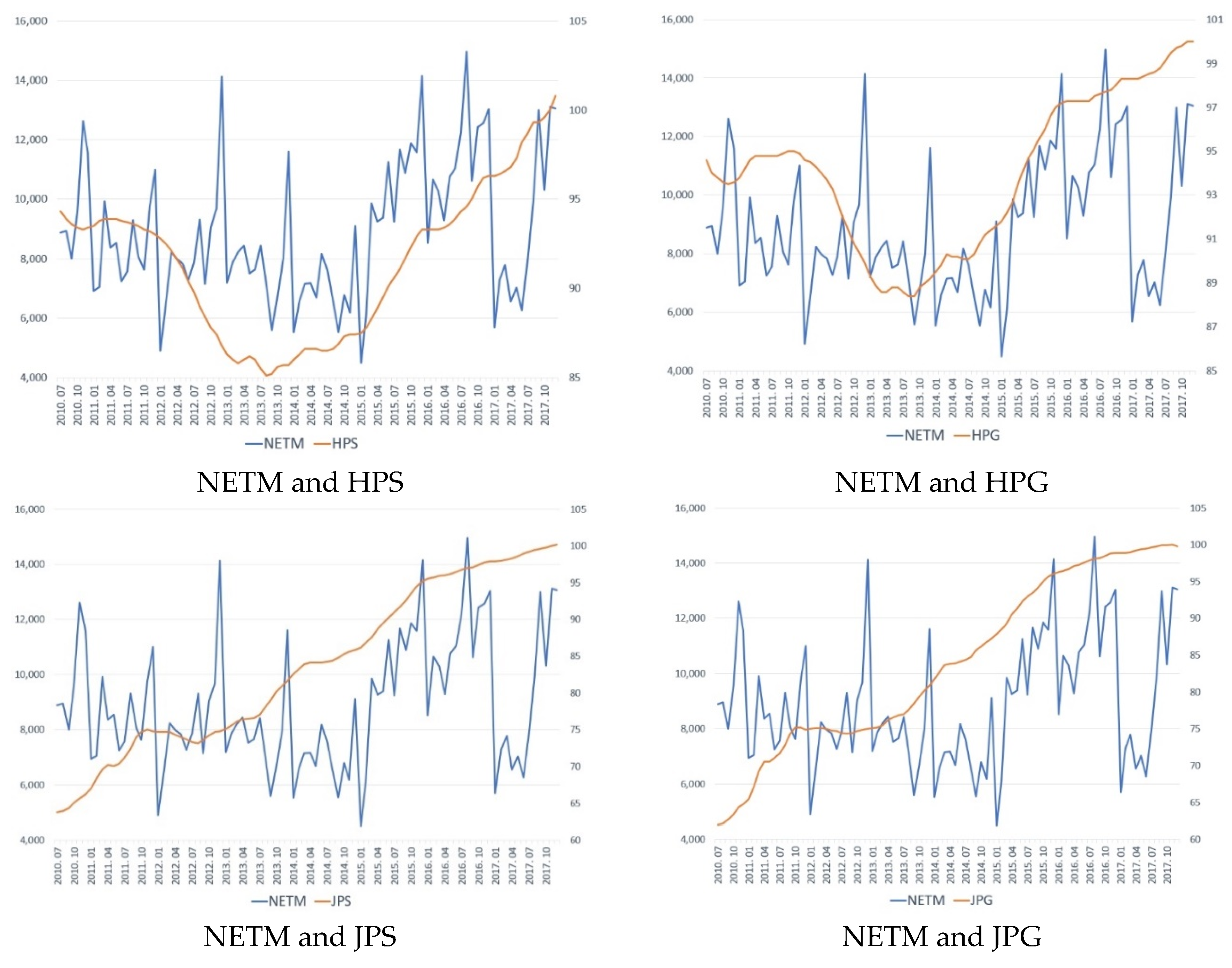
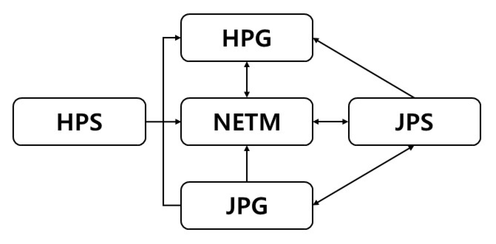
6.1. Relationship between Housing Markets and Residential Migration

This study used Granger causality analysis to find the relationship between residential migration and housing markets in the metropolitan area, the relationship between the housing markets of Seoul and Gyeonggi province, and the relationship between residential migration and demand–supply factors. The results showed that housing markets and residential migration had close causality (see

Table 5. Results of Granger causality test.

Null Hypothesis	lag 1		lag 2		lag 4		lag 6
	F	Prob.	F	Prob.	F	Prob.	F	Prob.
HPS ↛ NETM	8.999	0.004	3.817	0.026	3.374	0.014	2.280	0.018
NETM ↛ HPS	0.266	0.608	1.189	0.310	1.188	0.323	1.021	0.419
HPG ↛ NETM	3.434	0.067	3.563	0.0329	2.465	0.052	2.070	0.068
NETM ↛ HPG	0.420	0.519	2.837	0.065	1.965	0.109	1.098	0.373
JPS ↛ NETM	4.460	0.038	3.117	0.049	2.002	0.103	1.083	0.382
NETM ↛ JPS	0.006	0.937	2.511	0.088	2.553	0.046	2.330	0.042
JPG ↛ NETM	3.141	0.080	3.130	0.049	1.448	0.227	1.079	0.384
NETM ↛ JPG	0.037	0.848	1.322	0.272	0.919	0.458	1.323	0.259
HPS ↛ JPG	0.666	0.417	0.701	0.499	1.167	0.332	0.829	0.551
JPG ↛ HPS	1.529	0.220	0.897	0.412	0.612	0.655	0.743	0.617
HPG ↛ JPS	0.997	0.321	1.369	0.260	0.326	0.860	0.568	0.755
JPS ↛ HPG	5.199	0.025	3.525	0.034	0.954	0.438	0.785	0.585
HPS ↛ HPG	15.605	0.000	7.992	0.001	3.289	0.015	2.756	0.019
HPG ↛ HPS	0.000	0.988	0.633	0.534	0.085	0.987	0.865	0.525
JPS ↛ JPG	15.389	0.000	11.343	0.000	4.717	0.002	3.097	0.009
JPG ↛ JPS	0.345	0.559	6.700	0.002	2.554	0.046	1.800	0.112
HPS ↛ JPS	1.516	0.222	0.793	0.456	0.196	0.940	0.534	0.781
JPS ↛ HPS	0.523	0.471	1.568	0.215	0.626	0.645	1.234	0.300
HPG ↛ JPG	0.195	0.660	0.199	0.820	0.775	0.545	0.322	0.923
JPG ↛ HPG	3.199	0.077	1.663	0.196	0.903	0.467	0.862	0.527
NETM ↛ IND	27.197	0.000	5.993	0.004	4.389	0.003	5.982	0.000
IND ↛ NETM	57.574	0.000	20.959	0.000	16.171	0.000	15.121	0.000
NETM ↛ RATE	0.016	0.901	0.152	0.859	1.933	0.114	1.774	0.117
RATE ↛ NETM	0.018	0.892	1.200	0.306	1.199	0.318	2.390	0.037
NETM ↛ CONS	1.735	0.191	4.818	0.011	2.056	0.095	1.452	0.208
CONS ↛ NETM	10.191	0.002	4.351	0.016	1.147	0.341	1.214	0.310
NETM ↛ CONG	0.630	0.430	1.908	0.155	1.811	0.136	1.255	0.290
CONG ↛ NETM	0.113	0.738	0.685	0.507	1.712	0.156	1.352	0.246

Note: Bold denotes rejection of the hypothesis at the 0.10 (10%) level.

). Specifically, HPS and HPG had Granger causality to NETM throughout the entire period (lag 1 to 6). In contrast, however, NETM did not have a consistent effect on the housing sales market. Specifically, there was no causal relationships for HPS while HPG contributed to the NETM. This indicates that fluctuations in sales prices in Seoul and Gyeonggi province cause residential migration from Seoul to Gyeonggi, and this residential migration may also affect the housing sales market in Gyeonggi province accordingly.

As for the jeonse market, JPS and NETM had mutual causality. In other words, changes in jeonse prices in Seoul caused residential migration from Seoul to Gyeonggi province, which again caused fluctuations in jeonse prices in Seoul. On the other hand, JPG affected NETM but NETM did not have a significant effect on JPG. This indicates that changes in jeonse prices in Seoul may cause residential migration to Gyeonggi province, and changes in jeonse prices in Gyeonggi will also cause the same phenomenon. In other words, if jeonse residents in Seoul face difficulties due to fluctuations of jeonse prices in Seoul, they may move to Gyeonggi province because of the price changes in the Gyeonggi jeonse market.

These show that price changes in the Seoul housing market cause residential migration regardless of whether they are sales prices or jeonse prices, and residential migration from Seoul to Gyeonggi province Granger-causes changes in the Gyeonggi sales market, not the jeonse market. This proves that Seoul residents moving to Gyeonggi province are more interested in the sales market than the jeonse market in the short run. Additionally, the results found that residential migration from Seoul to Gyeonggi has the attribute of a ripple effect because of changes in Seoul housing market conditions.

Next, the relationship between housing markets in Seoul and Gyeonggi confirmed that the Seoul sales market was typically independent. However, the Gyeonggi sales market was affected by Seoul significantly and was subordinate to the Seoul sales market. For the jeonse market, JPS Granger-caused HPG and JPG throughout the entire period, proving that the Gyeonggi sales market was subordinate to the Seoul jeonse market. However, the Gyeonggi jeonse market was also partially affecting the Seoul jeonse market in the medium run. Thus, jeonse residents were sensitive to jeonse prices of both Seoul and Gyeonggi province. Moreover, there was no mutual Granger causality between HPS and JPS, which found distinct independence between the sales market and the jeonse market in Seoul. However, JPG showed causality to HPG, indicating that Gyeonggi sales prices may be affected by Gyeonggi jeonse prices.

This shows that the Seoul housing market typically maintains independence and affects the nearby Gyeonggi housing market. Specifically, the Seoul sales market affects the Gyeonggi sales market, and the Seoul jeonse market affects the Gyeonggi jeonse market, implying that there is high causality between housing markets of the same type.

By determining the effects of macroeconomic changes on residential migration, this study found that IND Granger-caused NETM with statistical significance. Also, RATE was a factor affecting NETM, which proved that residential migration was closely related to economic conditions. CONS was a cause of immediate residential migration, which subsequently affected CONS. However, CONG did not form a significant relationship with residential migration, which indicates that Seoul residents do not consider housing supply in Gyeonggi province a motive for residential migration.

In summary, the results of the Granger causality analysis imply that intra-metropolitan residential migration may occur due to changes in housing market conditions rather than playing a role in changing housing market conditions. In other words, residents living in Seoul would prefer to continue living there; however, they are forced to choose residential migration due to price changes in the Seoul housing market. Jeonse residents in Seoul, particularly, tend to move to Gyeonggi sales and the jeonse markets instead of staying in Seoul because of increasing jeonse prices. This residential migration is not to seek better housing but is an involuntary movement due to excessive residential costs in Seoul. This result implies that residential migration in the metropolitan area of South Korea is an involuntary ripple effect creating housing refugees.

6.2. Factors Affecting Intra-metropolitan Migration and Housing Markets

This study conducted a time series analysis to determine whether changes in the Seoul housing market conditions cause residential migration to surrounding areas and the time series effect this phenomenon has on surrounding area housing markets. Prior to this analysis, this study used the Johansen cointegration test to determine whether there is a stable time series relationship among the individual time series variables. The result showed that trace statistics rejected the null hypothesis that there was no cointegration relationship at the 5% significance level, thereby confirming that even though individual variables have unit roots and are unstable, there is a cointegration relationship among them, forming a stable time series relationship (see

Table 6. Result of Johansen cointegration test.

Hypothesized No. of CE(s)	Eigenvalue	Trace Statistic	Critical Value (0.05)	Prob.**
None *	0.727279	304.7564	69.81889	0.0001
At most 1 *	0.585915	194.3153	47.85613	0.0000
At most 2 *	0.469870	119.3720	29.79707	0.0000
At most 3 *	0.357945	65.42827	15.49471	0.0000
At most 4 *	0.278673	27.76635	3.841466	0.0000

Note 1: Trace test indicates five cointegrating eqn(s) at the 0.05 level. Note 2: * denotes rejection of the hypothesis at the 0.05 (5%) level. Note 3: ** MacKinnon–Haug–Michelis (1999) p-values.

). Thus, this study conducted an empirical analysis using the VECM, which is a limited form of the VAR model.

To determine the factors affecting residential migration in the metropolitan area and housing market changes, this study used housing market factors (HPS, JPS, HPG, and JPG) and NETM. The order of variables for analysis was HPS, JPG, HPG, JPS, and NETM, considering the Granger causality analysis results (see Figure 4) and the importance of variables for the research purpose. Specifically, NETM was arranged last so that the impact of other variables appeared first, to obtain significant results of impulse response and forecast error variance decomposition analysis on the target variables.

In addition, to choose the model that determines the VECM lag length, the optimal time lag was verified by applying the standards by Asghar and Abid [43] and Liew [46]. As a result, lag order 3 was suggested as the optimal time lag for all AIC, FPE, and HQ (see

Table 7. Result of vector autoregressive (VAR) lag order selection criteria.

Lag	LogL	LR	FPE	AIC	SC	HQ
0	−740.8541	NA	28.79291	17.54951	17.69319*	17.60730
1	−695.8371	83.67873	17.99890	17.07852	17.94063	17.42529
2	−659.4946	63.27867	13.86754	16.81164	18.39218	17.44738
3	−619.4859	64.95536*	9.892959*	16.45849*	18.75746	17.38320*

Note: * indicates lag order selected by the criterion. LR: sequential modified LR test statistic (each test at the 5% level). FPE: Final prediction error. AIC: Akaike information criterion. SC: Schwarz information criterion. HQ: Hannan-Quinn information criterion.

). Thus, this study set the ultimate optimal time lag as lag order 3.

The fit of the VECM model showed that for adj. R-square representing explanatory power, the previous housing market and residential migration factors explained 87% of the current residential migration and 31% to 51% of the current housing markets in Seoul and Gyeonggi province. Accordingly, the determinants affecting residential migration and changes in housing market conditions were sufficiently verified by the results of this study. The coefficients refer to the estimated coefficients, standard errors, and t-statistics, which show the short run impact (see

Table 8. Analysis result of vector error correction model (VECM).

Error Correction:	HPS	JPG	HPG	JPS	NETM
CointEq1	0.010707	−0.474237	0.017300	−0.338478	6074.437
	(0.08417)	(0.11045)	(0.06353)	(0.10226)	(925.085)
	[0.12720]	[−4.29377]	[0.27232]	[−3.30982]	[6.56635]
HPS(−3)	−0.444233	0.050715	−0.037044	0.083502	1011.284
	(0.17219)	(0.22595)	(0.12996)	(0.20921)	(1892.48)
	[−2.57988]	[0.22445]	[−0.28504]	[0.39913]	[0.53437]
JPG(−3)	−0.065100	−0.323307	−0.152422	0.054855	−6363.858
	(0.12702)	(0.16668)	(0.09587)	(0.15433)	(1396.07)
	[−0.51250]	[−1.93970]	[−1.58987]	[0.35544]	[−4.55842]
HPG(−3)	−0.120422	−0.239624	−0.142759	−0.294372	6726.647
	(0.21717)	(0.28497)	(0.16391)	(0.26386)	(2386.87)
	[−0.55450]	[−0.84087]	[−0.87096]	[−1.11564]	[2.81819]
JPS(−3)	0.172822	0.283449	0.205396	−0.142802	2944.945
	(0.13419)	(0.17608)	(0.10128)	(0.16304)	(1474.84)
	[1.28788]	[1.60974]	[2.02800]	[−0.87588]	[1.99679]
NETM(−3)	4.42E−07	−5.20E−05	−4.60E−06	−3.96E−05	−0.160789
	(9.4E−06)	(1.2E−05)	(7.1E−06)	(1.1E−05)	(0.10339)
	[0.04697]	[−4.20985]	[−0.64769]	[−3.46915]	[−1.55519]
C	−0.000960	−0.001988	−0.007500	−0.001923	20.31237
	(0.02514)	(0.03299)	(0.01897)	(0.03054)	(276.282)
	[−0.03818]	[−0.06026]	[−0.39529]	[−0.06297]	[0.07352]
Adj. R-squared	0.306560	0.507830	0.438286	0.340487	0.870657
F-statistic	3.293317	6.352552	5.047625	3.678153	35.91918
Log likelihood	13.70771	−9.114787	37.34339	−2.648768	−767.8951
Akaike AIC	0.078388	0.621781	−0.484366	0.467828	18.68798

Note: Standard errors in ( ) and t-statistics in [ ].

).

By examining the analysis results with a focus on lag order 3, which is the optimal time lag, this study found that NETM was closely related to changes in housing market conditions. In particular, the regression coefficients of housing markets in Seoul and Gyeonggi province were opposite, indicating that the two housing markets had opposite effects on residential migration. Specifically, the rise in housing sales prices and jeonse prices in Seoul ultimately increased NETM. On the other hand, the rise in jeonse prices in Gyeonggi reduced NETM. As previously explained, involuntary residential migration due to increases in housing sales and jeonse prices in Seoul may be concentrated in Gyeonggi province, which is why the rise in jeonse prices in Gyeonggi offsets the motivation for residential migration, thereby reducing the ripple effect. However, HPG served as a factor that had a positive effect on NETM in the short run, which indicates that when there is a price increase in the housing sales market in Gyeonggi, Seoul residents tend to seek economic benefit through housing purchases in Gyeonggi province in the short run. This was also verified by the Granger causality analysis. To determine more tangible proof, it is necessary to verify the long-term trend through impulse response analysis and forecast error variance decomposition analysis.

Next, this study determined housing market and residential migration factors that affect housing markets and found that housing sales and jeonse markets in both Seoul and Gyeonggi province did not have high statistical significance in the short run. In this sense, it was necessary to examine the factors affecting housing markets over the long term. Regardless of the statistical significance, the short-run relationship of each housing market shows that HPS had a negative correlation with Gyeonggi housing markets (HPG, JPG) and a positive correlation with JPS, while JPS had a positive correlation with HPS and JPG and a negative correlation with HPG. HPG had a positive correlation with HPS and JPG, while it had the opposite correlation with JPS, and JPG had a positive correlation with HPS and JPS and a negative correlation with HPG.

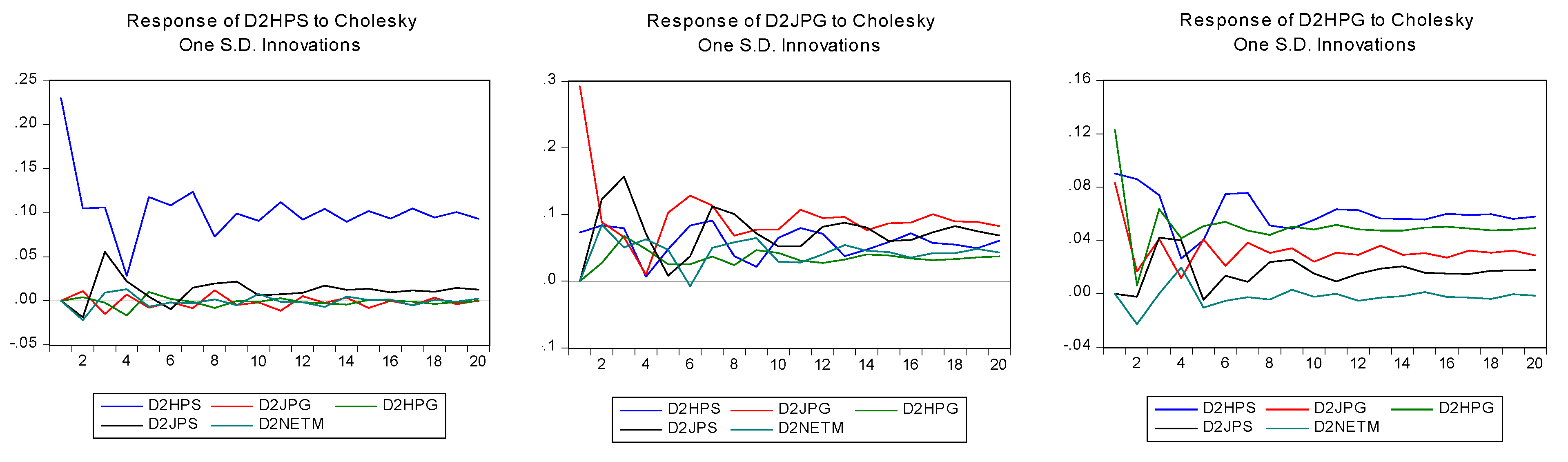
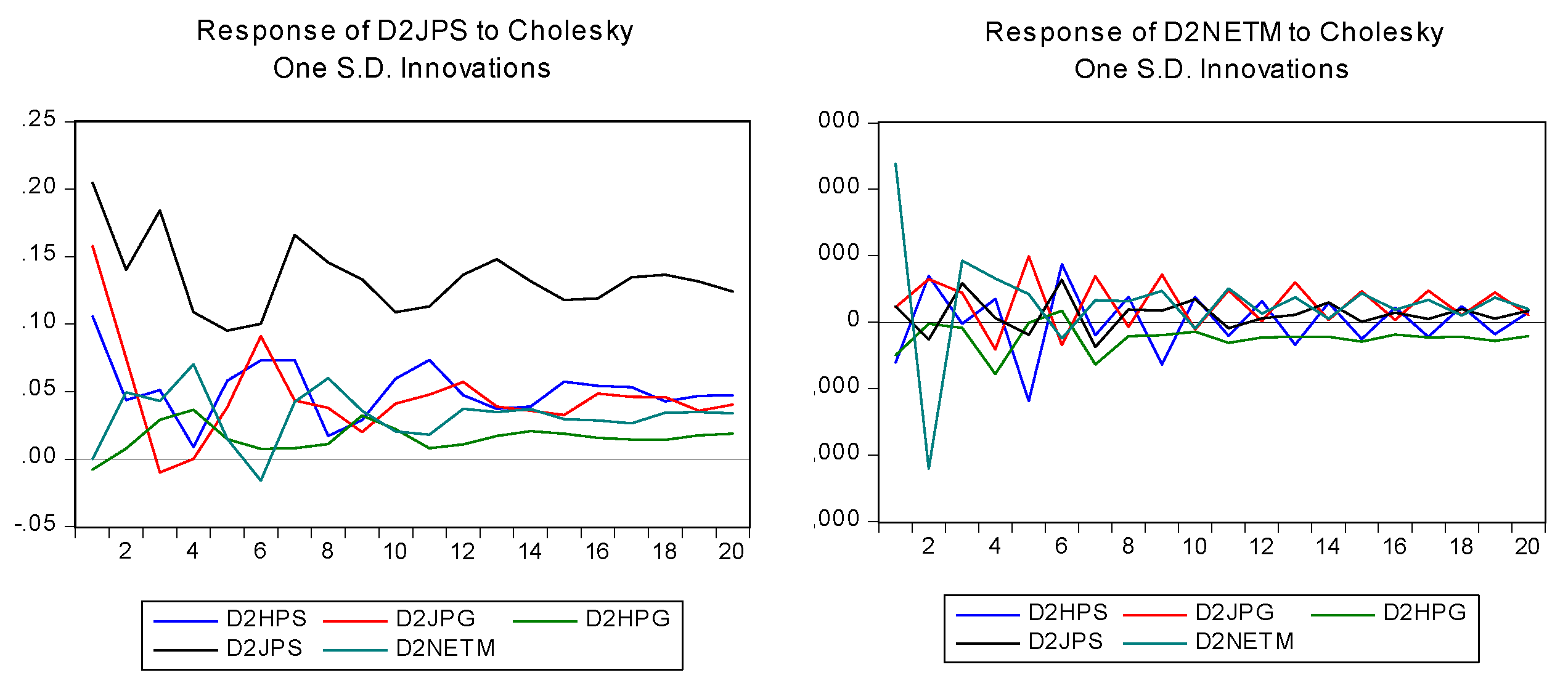
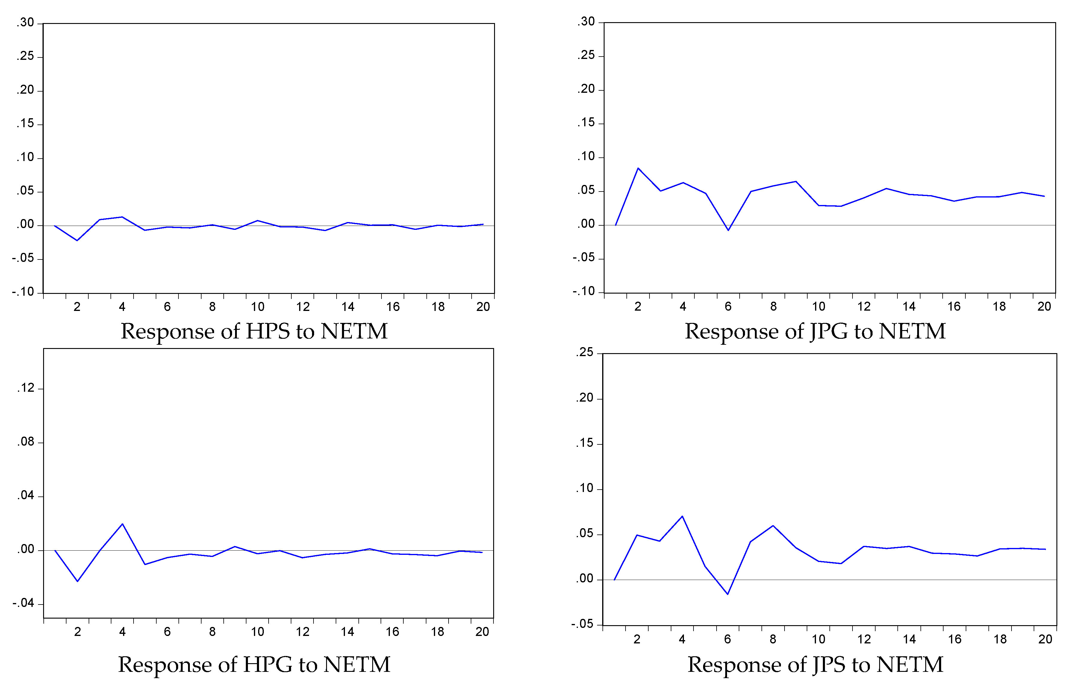
6.3. Impulse Response Analysis

This study examined the short and long-run time series effects of the shock of residential migration on housing markets based on the impulse response analysis. Specifically, this study checked the responses of all variables in the model toward the unit impulse to the extent of each variable’s standard deviation as time passes up to 20 periods. This study then verified how the changes in the housing market (HPS, HPG, JPS, JPG) conditions and NETM impact NETM and housing markets, respectively, by the response of residential migration to housing markets and the response of housing markets to residential migration.

The result verified that the factor with the greatest impact on HPS was HPS itself, which increased the sales price index through the entire period by at least 0.1 point, on average. Then, the factor that had the next biggest impact was JPS, which has had a constant impact on HPS since period 2. The reason that JPS has a significant influence over HPS is because South Korean property owners typically increase the deposit amount when renewing a jeonse contract. Thus, the jeonse prices approach the sales prices. In this case, the tenant either pays the increased jeonse deposit and continues to live in the property as a jeonse tenant or considers buying a house. Therefore, the jeonse prices have a significant impact on housing sales prices. JPS was also most greatly affected by its own change. However, the factor that had the next most important impact varied depending on time; JPG had a great impact in the short run and HPS in the medium run. On the other hand, HPG showed a different pattern from the Seoul housing market. Also, HPS had the strongest impact on the Gyeonggi sales market, except for the initial period. Similarly, JPG was significantly affected by JPS up to the medium run.

For NETM, the effect from changes in residential migration itself was significant at first, but in the medium run, JPG had a significant effect on residential migration (see Figure 5). Both HPS and JPS had a significant effect on NETM from the initial to the medium run, but the impact on residential migration afterward was limited. On the other hand, HPG caused an increase in NETM at first because Seoul residents pursued economic benefit through housing purchases in Gyeonggi province. However, due to the high prices, residential migration decreased later.

Next, the effects of residential migration on the housing markets of Seoul and Gyeonggi (see Figure 6) showed that NETM had an unstable effect on HPS and HPG in the short run, but had almost no effect in the long run. On the other hand, NETM had a great impact on the Seoul and Gyeonggi jeonse markets in the short run, which indicates that residential migration was concentrated in the Gyeonggi jeonse market and resulted in a rise in jeonse prices. The Seoul jeonse market also had high causality with residential migration, but the Gyeonggi jeonse market also showed an increase in prices. This implies that the increased housing expenses in Seoul forced residents to move to the relatively less expensive Gyeonggi jeonse market, but this resulted in increasing Gyeonggi jeonse prices.

These results show that Seoul and Gyeonggi province have different housing market characteristics. While the Seoul housing market tends to be independent from Gyeonggi province, the Gyeonggi housing market is strongly subordinate to Seoul’s housing market. This finding indicates that a ripple effect is likely, by which changes in the Seoul housing market will be easily transmitted to the Gyeonggi housing market. This study verified that residential migration from Seoul to Gyeonggi province is not to seek a stable residential environment but is involuntary migration due to the financial burden of increased housing costs in Seoul. This study also confirmed that there may be a ripple effect that intensifies instability in the jeonse market due to residential migration from Seoul to Gyeonggi province.

6.4. Forecast Error Variance Decomposition Analysis

This study conducted forecast error variance decomposition analysis to determine how much the forecast error variance of residential migration and housing markets is explained by the variable itself and other variables. It was found that HPS itself had an explanatory power of at least 96% and explained the housing sales market in Seoul throughout the entire period. In other words, changes in the Seoul sales market conditions were not caused by external factors but rather by the shock of the housing sales market, which shows the independent character of the market. JPS explained as much as 70% of its own shock in the long run. However, unlike the housing sales market that was independent, 12.2% was explained by the shock of JPG, indicating that there may be a relatively active ripple effect between the jeonse markets in the metropolitan areas (see

Table 9. Variance decomposition of housing markets and residential migration.

Period	HPS					JPS					HPG
	HPS	JPG	HPG	JPS	NETM	HPS	JPG	HPG	JPS	NETM	HPS	JPG	HPG	JPS	NETM
1	100.00	0.00	0.00	0.00	0.00	14.40	31.87	0.08	53.66	0.00	26.98	22.94	50.08	0.00	0.00
2	98.49	0.18	0.03	0.55	0.75	12.20	28.29	0.11	57.12	2.28	40.47	18.74	39.42	0.01	1.37
3	94.52	0.44	0.03	4.30	0.72	10.72	20.80	0.66	64.91	2.92	40.91	17.31	37.31	3.45	1.02
4	93.43	0.50	0.38	4.79	0.91	9.59	18.50	1.39	64.92	5.59	38.83	16.14	37.36	6.03	1.64
5	94.16	0.49	0.43	4.11	0.82	10.70	17.85	1.40	64.77	5.27	37.68	17.27	37.91	5.48	1.65
6	94.70	0.44	0.38	3.74	0.74	12.07	19.81	1.27	62.08	4.77	40.71	15.66	37.12	5.04	1.48
7	95.13	0.44	0.34	3.44	0.65	12.46	17.58	1.10	64.07	4.79	43.00	15.63	35.52	4.54	1.31
8	94.89	0.53	0.37	3.58	0.62	11.32	16.36	1.04	65.62	5.66	43.00	15.61	35.28	4.87	1.24
9	94.90	0.51	0.34	3.65	0.60	10.78	15.29	1.32	66.93	5.68	42.44	15.73	35.46	5.22	1.16
10	95.11	0.48	0.33	3.47	0.60	11.30	14.94	1.41	66.87	5.49	42.87	15.33	35.58	5.12	1.09
11	95.38	0.52	0.31	3.23	0.56	12.23	14.68	1.34	66.51	5.24	43.52	15.11	35.51	4.83	1.02
12	95.55	0.51	0.29	3.12	0.53	11.98	14.54	1.27	66.96	5.25	44.15	14.88	35.27	4.72	0.97
13	95.63	0.49	0.28	3.08	0.52	11.51	13.93	1.26	68.09	5.21	44.20	15.08	35.06	4.74	0.92
14	95.71	0.47	0.28	3.03	0.51	11.26	13.48	1.30	68.69	5.26	44.36	14.96	34.99	4.82	0.88
15	95.81	0.48	0.26	2.96	0.49	11.52	13.12	1.32	68.81	5.23	44.44	14.90	35.06	4.76	0.84
16	95.94	0.46	0.25	2.88	0.47	11.65	13.04	1.32	68.82	5.17	44.75	14.67	35.09	4.69	0.80
17	96.06	0.45	0.24	2.80	0.46	11.66	12.82	1.29	69.17	5.06	44.94	14.67	35.01	4.61	0.77
18	96.16	0.44	0.24	2.73	0.44	11.46	12.63	1.27	69.59	5.05	45.18	14.62	34.88	4.59	0.74
19	96.23	0.42	0.23	2.70	0.42	11.39	12.33	1.28	69.94	5.07	45.22	14.65	34.83	4.59	0.71
20	96.30	0.41	0.22	2.67	0.41	11.37	12.15	1.30	70.10	5.08	45.35	14.54	34.84	4.59	0.68
Period	JPG					NETM
	HPS	JPG	HPG	JPS	NETM	HPS	JPG	HPG	JPS	NETM
1	5.90	94.10	0.00	0.00	0.00	5.75	0.79	3.86	0.84	88.76
2	9.60	72.53	0.59	11.73	5.55	6.93	3.82	2.02	1.02	86.21
3	10.90	57.11	3.12	23.19	5.67	6.23	4.84	1.87	3.41	83.65
4	10.24	53.57	4.20	24.50	7.49	6.48	5.53	5.79	3.13	79.07
5	10.59	54.63	4.19	22.58	8.01	13.54	10.29	4.93	2.87	68.36
6	12.50	55.75	4.01	20.63	7.12	16.55	10.17	4.73	4.82	63.72
7	13.87	52.65	3.95	22.47	7.06	15.78	11.96	6.47	5.23	60.56
8	13.38	50.52	3.88	24.46	7.76	16.23	11.79	6.58	5.33	60.07
9	12.74	49.48	4.37	24.71	8.69	17.21	13.48	6.40	5.17	57.74
10	13.45	48.93	4.73	24.36	8.53	17.62	13.35	6.40	5.64	56.99
11	14.45	49.09	4.70	23.56	8.21	17.31	13.99	6.65	5.52	56.53
12	14.92	48.43	4.61	23.90	8.13	17.61	13.88	6.83	5.49	56.18
13	14.42	48.02	4.61	24.51	8.43	17.61	15.01	6.84	5.38	55.16
14	14.33	47.30	4.81	25.00	8.57	17.80	14.87	6.98	5.70	54.65
15	14.54	47.07	4.96	24.79	8.65	17.66	15.42	7.18	5.57	54.18
16	15.08	46.78	5.01	24.57	8.56	17.75	15.33	7.28	5.62	54.01
17	15.09	46.78	4.99	24.59	8.55	17.63	15.97	7.37	5.53	53.50
18	15.07	46.43	5.00	24.95	8.55	17.74	15.91	7.52	5.64	53.19
19	14.96	46.20	5.06	25.10	8.68	17.56	16.40	7.70	5.56	52.78
20	15.14	45.87	5.15	25.11	8.73	17.55	16.36	7.83	5.64	52.63

Note: Cholesky ordering is HPS JPG HPG JPS NETM.

).

On the other hand, the Gyeonggi housing market showed relatively little change caused by the shock of its own variable compared to Seoul. For HPG, the explanatory power of its own shock that exceeded 50% in the short run (period 1) dropped to less than 35% in the long run (period 20). In the process, the impact of HPS became significantly stronger, and the part where HPS explains HPG became greater than the part explained by its own shock after period 2. The fact that the Seoul sales market contributed substantially to the changes in the Gyeonggi sales market indicates that there may be a subordinate ripple effect by which changes in housing sales prices in Seoul can be directly reflected in the housing sales prices in Gyeonggi even without residential migration. JPG explained 25% of its own shock, although the dependency was lower than HPG, showing that there is a ripple effect. The part explained by the shock of NETM on JPG was also 9% in the long run, which is remarkably higher than HPS, JPS, and HPG.

Finally, 89% of NETM was explained by the shock of residential migration in the short run and 53% in the long run, showing that residential migration causes additional residential migration. However, a relatively large part was explained by housing markets in the long run, particularly HPS and JPG, which explained 34% of residential migration. This indicates that changes in sales prices in Seoul and in jeonse prices in Gyeonggi may be the main cause of residential migration. As previously explained, increases in housing expenses in Seoul may be the cause of a ripple effect on the Gyeonggi jeonse market, which is a relatively inexpensive.

7. Conclusion and Findings

Recently, the housing market trend in South Korea has been shifting and moving toward operating profits, such as rent, instead of capital gains from profit margins on purchases and sales. In the process, jeonse, a type of housing lease unique to South Korea, has undergone price increases due to demand–supply imbalance in Seoul. Sales prices are so high that it is impossible for people to purchase a house by merely saving up, which adds to the difficulty of living in Seoul. Therefore, residential migration to Gyeonggi province, adjacent to Seoul, is increasing, as residents cannot afford the increased jeonse and sales prices. In this regard, the housing markets in Seoul and Gyeonggi are undergoing a great change. This study examined the relationship between housing markets and residential migration in the Seoul metropolitan area. The study also reviewed whether there was a housing refugee phenomenon due to an involuntary ripple from this process.

The Granger causality analysis proved that changes in housing market conditions in Seoul are causing residential migration to Gyeonggi province regardless of sales or jeonse. Moreover, the Seoul housing market generally maintains independence while affecting the Gyeonggi housing market. In particular, the Seoul jeonse market has a significant ripple effect on both the sales and jeonse markets in Gyeonggi. Next, through VECM, impulse response analysis, and variance decomposition analysis, this study proved once again that the Gyeonggi housing market is subordinate to Seoul and is greatly affected by Seoul in terms of both sales and jeonse prices. Thus, changes in sales and jeonse prices in Seoul are a major cause of residential migration to Gyeonggi province.

In conclusion, this study confirmed that Seoul and Gyeonggi province have different characteristics concerning their housing market conditions. While the Seoul housing market tends to be independent from Gyeonggi province, the Gyeonggi housing market is strongly subordinate to Seoul. This indicates that a ripple effect is likely to occur by which any changes in the Seoul housing market conditions will be easily transmitted to the Gyeonggi housing market. This study also found that intra-metropolitan residential migration may occur due to changes in housing market conditions, rather than playing a role in changing housing market conditions, and residential migration from Seoul to Gyeonggi province is not for the purpose of seeking a stable residential environment, but it is involuntary migration caused by the financial burden of increased housing costs in Seoul. This study confirmed that there may be a ripple effect that intensifies instability in the jeonse market due to residential migration from Seoul to Gyeonggi province. This study clearly showed that residential migration occurring in the Seoul metropolitan area is an involuntary ripple effect—a housing refugee phenomenon.

Finally, the study results, which prove that changes in housing market conditions cause a ripple effect on the surrounding areas, showed that residential migration in Seoul affects the Gyeonggi housing market, particularly the jeonse market, which causes a series of residential migration events to housing markets in peripheral areas that are farther away from Gyeonggi province, thereby causing the spread of an involuntary ripple effect. This seems to influence reflationary measures by activating housing transactions. However, considering that this residential migration is involuntary, there is a concern that jeonse refugees may spread out to small and medium cities beyond the metropolitan area. For this reason, housing policy for metropolitan areas in South Korea must focus on providing physical and financial support to maintain residential stability in large cities such as Seoul to prevent the refugee phenomenon, whereby residents are forced to involuntarily move to other regions. Considering the sequential ripple effect of changes in housing market conditions in the Seoul metropolitan area, policymakers should also consider the need for a housing management policy that can comprehensively manage housing markets in multiple regions. Our findings illustrate the direction of housing policy for maintaining housing stability in countries where the population is concentrated in certain urban areas, such as metropolitan regions. A system which considers the aforementioned policy directions should be established, given that involuntary residential migration caused by housing instability in large cities will increase influx in the housing markets of nearby cities, which in turn could act as the cause of uncertainty and instability in the overall national housing market.

This study overcame the limitations of previous studies by reviewing how the changes in housing market conditions in Seoul and residential migration are causing a ripple effect on the surrounding housing markets. However, there may be a different ripple effect pattern in the housing markets of other city regions with different circumstances. In other words, residents may directly choose to migrate to housing markets in the Seoul metropolitan area instead of moving to a nearby low-tier housing market. Therefore, further research and a theoretical foundation would establish the direction for an integrated housing policy by verifying the patterns of the ripple effect depending on the characteristics of each city region. Moreover, this study contributes to the understanding of the relationship between residential migration and housing market conditions of countries in which the functions are concentrated in metropolitan areas, as they are in South Korea, and in which the central government proposes housing policy. However, there may be different patterns of ripple effects in countries where urban functions and housing policy authorities are dispersed. Therefore, conducting related research by considering these characteristics may be the foundation for understanding the ripple effect in a broader sense.

References

1. Ryu, K.; Kim, J. Jeonse, will it be extinguished? Differentiation of Korean rental housing market. J. Hous. Built Environ. 2018, 33, 409–427. [Google Scholar] [CrossRef]
2. Yoon, J. Structural changes in South Korea’s rental housing market: The rise and fall of the Jeonse system. J. Comp. Asian Dev. 2003, 2, 151–168. [Google Scholar] [CrossRef]
3. Ambrose, B.; Kim, S. Modeling the Korean chonsei lease contract. Real Estate Econ. 2003, 31, 53–74. [Google Scholar] [CrossRef]
4. Kim, S.; Kim, J.; Kim, J. Structural changes in the Korean housing market before and after macroeconomic fluctuations. Sustainability 2016, 8, 415. [Google Scholar] [CrossRef] [Green Version]
5. Jones, C.; Leishman, C. Spatial dynamics of the housing market: An interurban perspective. Urban Stud. 2006, 43, 1041–1059. [Google Scholar] [CrossRef]
6. Seo, W. Dynamic relationship between housing consumer sentiment in Seoul and metropolitan housing market. SH Urban Res. Insight 2019, 9, 31–47. [Google Scholar] [CrossRef]
7. Jeong, Y.; Kim, K.; Kim, H.; Yang, D.; Kang, E. A Diagnosis of Bubble Risk in the Global Real Estate Sector and Prospective Impacts on Financial Crises; Policy Analysis 18-01; Korea Institute for International Economic Policy: Seoul, Kerea, 2018. [Google Scholar]
8. Ashworth, J.; Parker, S. Modeling regional house prices in the UK. Scott. J. Political Econ. 1997, 44, 225–246. [Google Scholar] [CrossRef]
9. Cook, S.; Thomas, C. An alternative approach to examining the ripple effect in UK house prices. Appl. Econ. Lett. 2003, 10, 749–851. [Google Scholar] [CrossRef]
10. Cook, S.; Watson, D. A new perspective on the ripple effect in the UK housing market: Comovement, cyclical subsamples and alternative indices. Urban Stud. 2016, 53, 3048–3062. [Google Scholar] [CrossRef] [Green Version]
11. Giussani, B.; Hadjimatheou, G. Modeling regional house prices in the United Kingdom. Pap. Reg. Sci. 1991, 70, 201–219. [Google Scholar] [CrossRef]
12. Meen, G. Spatial aggregation, spatial dependence and predictability in the UK housing market. Hous. Stud. 1996, 11, 345–372. [Google Scholar] [CrossRef]
13. Meen, G. Regional house prices and the ripple effect: A new interpretation. Hous. Stud. 1999, 14, 733–753. [Google Scholar] [CrossRef]
14. Tsai, I. Ripple effect in house prices and trading volume in the UK housing market: New viewpoint and evidence. Econ. Model. 2014, 40, 68–75. [Google Scholar] [CrossRef]
15. Blake, J.; Gharleghi, B. The ripple effect at an inter-suburban level in the Sydney metropolitan area. Int. J. Hous. Mark. Anal. 2018, 11, 2–33. [Google Scholar] [CrossRef]
16. Ma, L.; Liu, C. Ripple effects of house prices: Considering spatial correlations in geography and demography. Int. J. Hous. Mark. Anal. 2013, 6, 284–299. [Google Scholar] [CrossRef] [Green Version]
17. Shi, S.; Young, M.; Hargreaves, B. The ripple effect of local housing price movements in New Zealand. J. Prop. Res. 2009, 26, 1–24. [Google Scholar] [CrossRef]
18. Pollakowski, H.O.; Ray, T.S. Housing price diffusion patterns at different aggregation level: An examination of housing market efficiency. J. Hous. Res. 1997, 8, 107–124. [Google Scholar]
19. Chiang, S. Housing markets in China and policy implications: Comovement or ripple effect. China World Econ. 2014, 22, 103–120. [Google Scholar] [CrossRef]
20. Huang, F.; Li, C.; Li, Y. Ripple effect of housing prices among Chinese deputy provincial cities based on an alternative approach. Int. J. Bus. Adm. 2010, 1, 19–24. [Google Scholar] [CrossRef] [Green Version]
21. Zhang, L.; Hui, E.C.; Wen, H. The regional house prices in China: Ripple effect or differentiation. Habitat Int. 2017, 67, 118–128. [Google Scholar] [CrossRef]
22. Suh, S. An empirical study on the existence and the cause of ripple effect: The case of Kangnam-gu. Seoul Study 2007, 8, 1–13. [Google Scholar]
23. Choi, K.; Hyung, N.; Jeon, H.; Kim, J. Analyzing the spillover effect of housing prices. In Proceedings of the 3rd International Conference on Humanities, Geography and Economics, Bali, Indonesia, 4–5 January 2013; pp. 138–142. [Google Scholar]
24. Jeon, H.; Hyung, N. Spillover effects in the housing market: Shocks originating from gangnam. Hous. Stud. Rev. 2018, 26, 63–88. [Google Scholar] [CrossRef] [Green Version]
25. Jin, C.; Lee, G. Analysis of the spatio-temporal interaction patterns of the house sales and rent price using SpVAR model: Focus on the Seoul metropolitan area. J. Real Estate Anal. 2016, 2, 23–42. [Google Scholar] [CrossRef]
26. Lee, H.; Lee, J. Spillover effects of apartment housing prices across cities: A generalized forecast error variance decomposition for seven large cities. Korea Spat. Plan. Rev. 2014, 82, 3–15. [Google Scholar]
27. Munro, M.; Mclennan, D. Intra-urban changes in house prices: Glasgow 1972–83. Hous. Stud. 1987, 2, 65–81. [Google Scholar] [CrossRef]
28. Wilson, P.; White, M.; Dunse, N.; Cheong, C.; Zurbruegg, R. Modelling price movements in housing micro market: Identifying long-term components in local housing market dynamics. Urban Stud. 2011, 48, 1853–1874. [Google Scholar] [CrossRef]
29. Macdonald, R. Regional house prices in Britain: Long-run relationships and short-run dynamics. Scott. J. Political Econ. 1993, 40, 43–55. [Google Scholar] [CrossRef]
30. Cook, S. Detecting long-run relationship in regional house prices in the UK. Int. Rev. Appl. Econ. 2005, 19, 107–118. [Google Scholar] [CrossRef]
31. Lee, C.; Chien, M. Empirical modeling of regional house prices and the ripple effect. Urban Stud. 2011, 48, 2029–2047. [Google Scholar] [CrossRef]
32. Chang, B. Spillover effect and its time-varying characteristics in the Korean housing market. Hous. Stud. Rev. 2014, 22, 5–30. [Google Scholar]
33. Kim, H. Spatio-temporal analysis of house price diffusion of Korea. J. Korean Econ. Anal. 2017, 23, 89–135. [Google Scholar]
34. Dickey, D.; Fuller, W. Distribution of the estimators for autoregressive time series with a unit root. J. Am. Stat. Assoc. 1979, 74, 427–431. [Google Scholar]
35. Harris, R.I.D. Testing for unit roots using the augmented dickey-fuller test. Econ. Lett. 1992, 38, 381–386. [Google Scholar] [CrossRef]
36. Granger, C. Investigating causal relations by econometric model and cross-spectral methods. Econometrica 1969, 37, 424–438. [Google Scholar] [CrossRef]
37. Han, Y.; Han, K.; Lee, J. A study on the causality of housing price variations. J. Korean Urban Manag. Assoc. 2010, 23, 199–219. [Google Scholar]
38. Schelter, B.; Winterhalder, M.; Timmer, J. Handbook of Time Series Analysis: Recent Theoretical Developments and Applications; Wiley-VCH: Weinheim, Germany, 2006. [Google Scholar]
39. Enders, W. Applied Econometric Time Series; Willey: Hobken, NJ, USA, 2014. [Google Scholar]
40. Sims, C. Macroeconomics and reality. Ecoometrica 1980, 48, 1–48. [Google Scholar] [CrossRef] [Green Version]
41. Engle, R.; Granger, C. Co-integration and error correction: Representation, estimation and testing. Econometrica 1987, 55, 251–276. [Google Scholar] [CrossRef]
42. Maysami, R.; Koh, T. A vector error correction model of the Singapore stock market. Int. Rev. Econ. Financ. 2000, 9, 79–96. [Google Scholar] [CrossRef]
43. Asghar, Z.; Abid, I. Performance of Lag Length Selection Criteria in Three Different Situations; MPRA Paper No. 40042; University Library of Munich: Munich, Germany, 2007; Available online: https://EconPapers.repec.org/RePEc:pra:mprapa:40042 (accessed on 13 July 2012).
44. Gallet, C. Housing market segmentation: An application of convergence tests to Los Angeles housing. Ann. Reg. Sci. 2002, 38, 551–561. [Google Scholar] [CrossRef]
45. Islam, K.; Asami, Y. Housing market segmentation: A review. Rev. Urban Reg. Dev. Stud. 2009, 21, 93–109. [Google Scholar] [CrossRef]
46. Liew, V. Which lag length selection criteria should be employ? Econ. Bull. 2004, 3, 1–9. [Google Scholar]
Figure 1. Housing market trends in the Seoul metropolitan area. Data source: Korea Appraisal Board.
Sustainability 12 01225 g001
Figure 2. Residential migration patterns in the Seoul metropolitan area. Data source: Korea Appraisal Board.
Sustainability 12 01225 g002
Figure 3. Residential migration and housing market trends in the Seoul metropolitan area. Data source: Korea Appraisal Board.
Sustainability 12 01225 g003
Figure 4. Relationship between housing markets and intra-metropolitan migration.
Sustainability 12 01225 g004
Figure 5. Results of impulse response analysis.
Sustainability 12 01225 g005aSustainability 12 01225 g005b
Figure 6. Impulse response of housing markets to NETM.
Sustainability 12 01225 g006