Detecting Possible Reduction of the Housing Bubble in Korea for Different Residential Types and Regions


Abstract
1. Introduction
2. Literature Review
3. Data & Methods
3.1. Data
- -
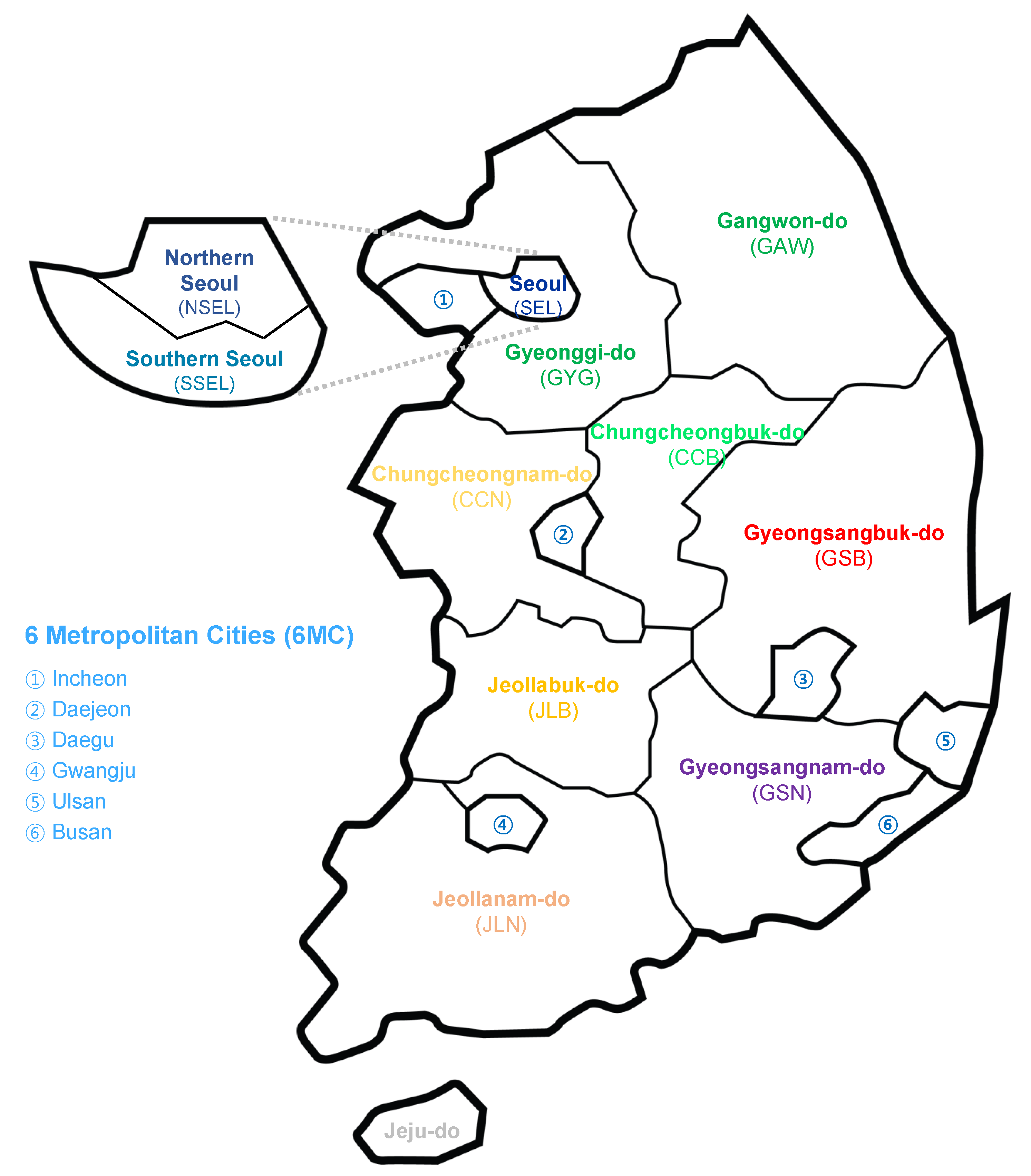
- SEL, NSEL, SSEL, 6MC, GYG, GAW, CCB, CCN, JLB, JLN, GSB, GSN, Non-Metropolitan Areas (NMA, all regions except the SEL, 6MC, and GYG)
- -
- SEL, NSEL, SSEL, 6MC, GYG, NMA
3.2. Real Options Framework
3.2.1. Arbitrage and Real Option Setting
3.2.2. Mechanics of the Binomial Option Pricing Model with Heteroscedasticity
- First stage: From the landlord’s Contract notice in the market to the Contract date.
- Second stage: From the Contract date to maturity of the Contract.
3.3. Data Exploration
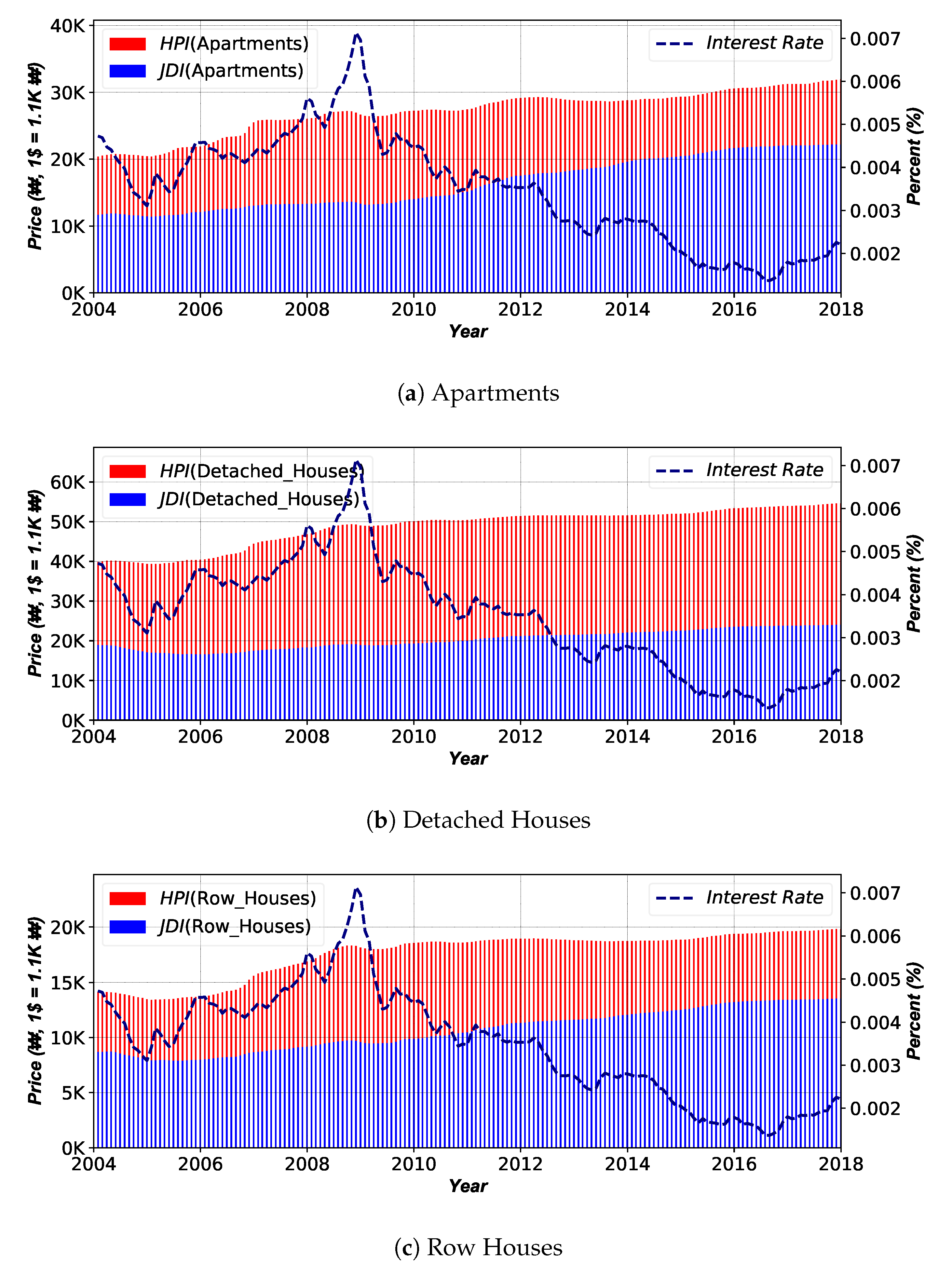
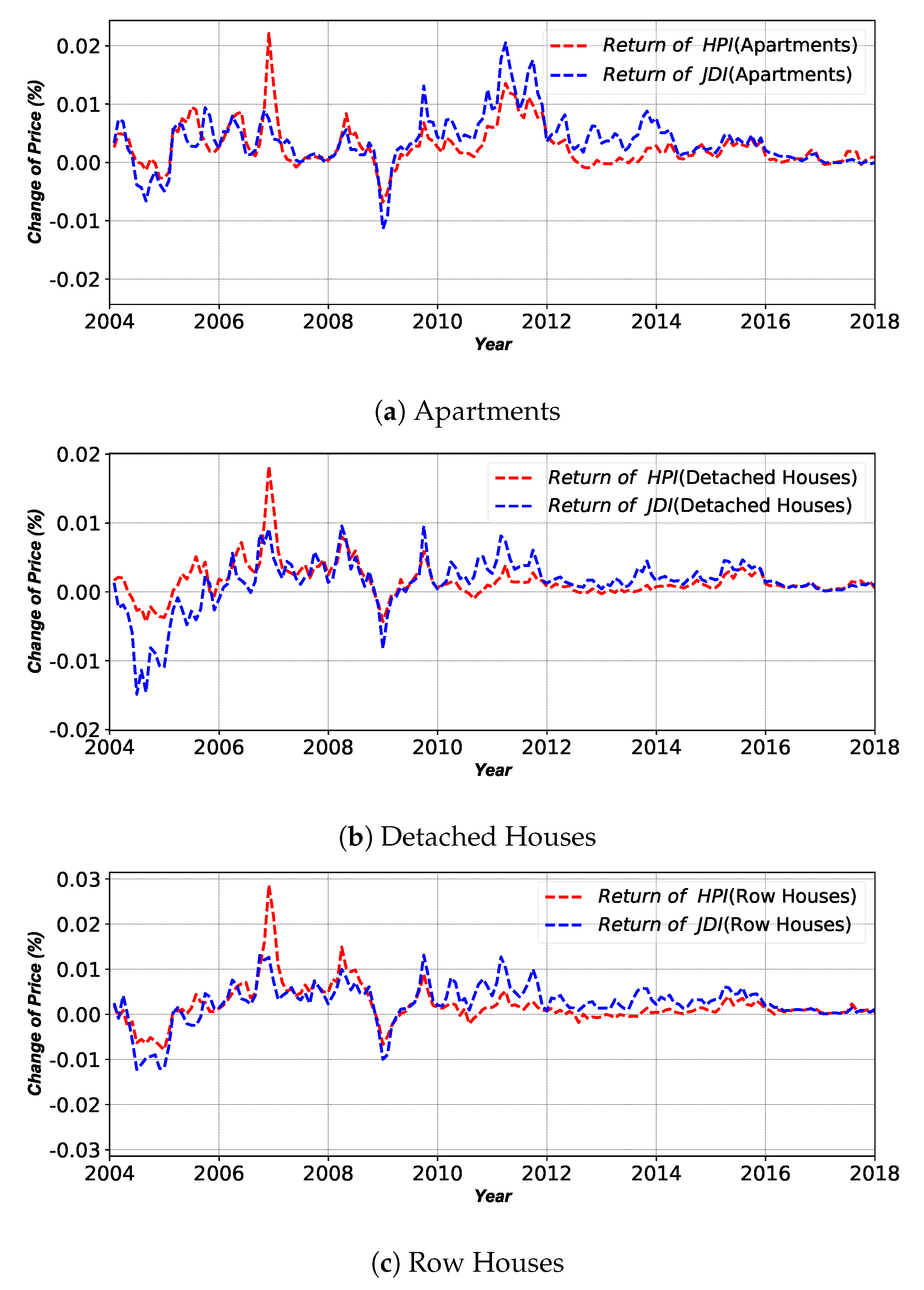
3.3.1. Indices and Spreads
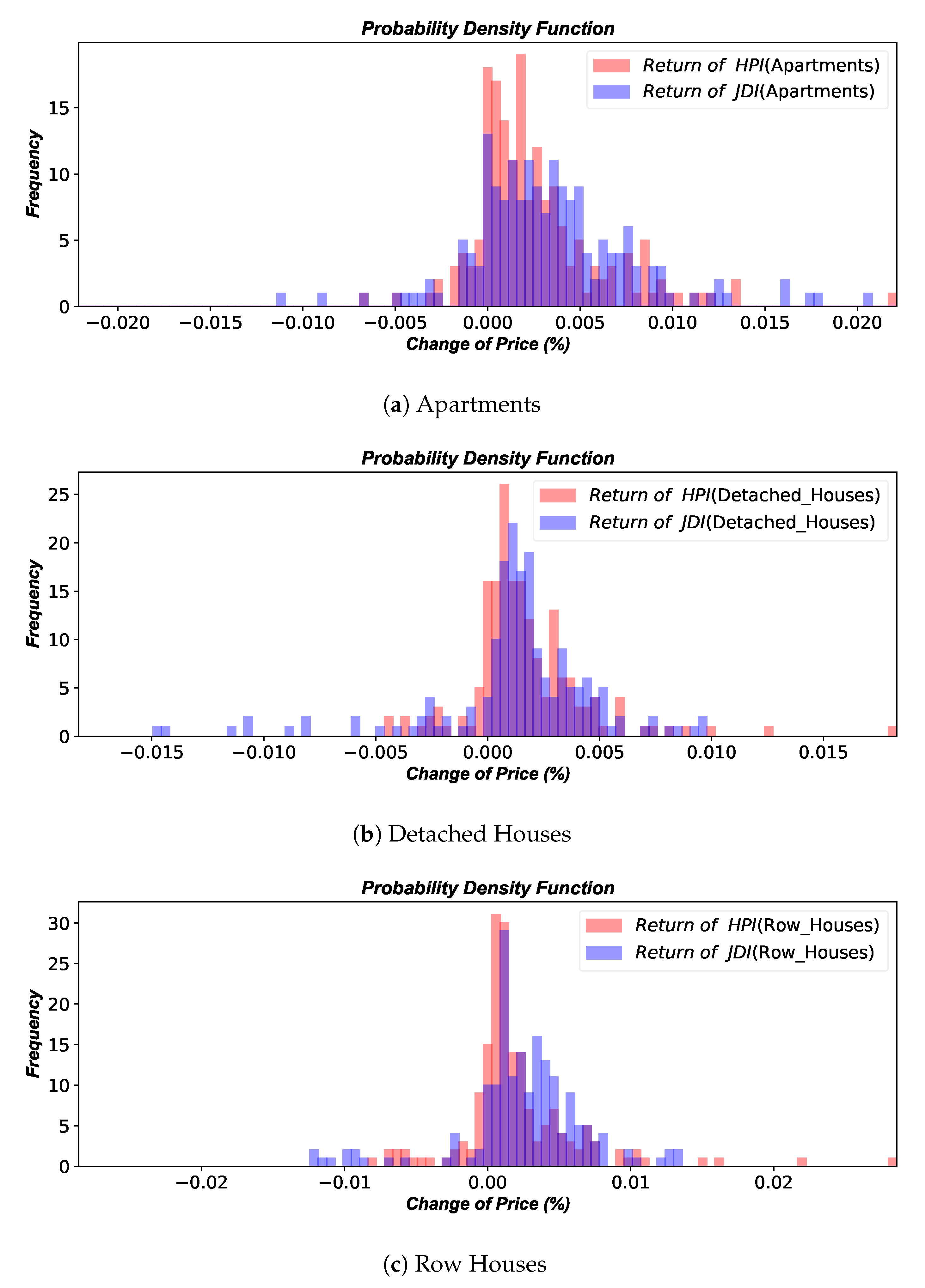
3.3.2. Existence of Heteroscedasticity in Returns
4. Results and Discussions
4.1. Analyses on Bubbles in Real Estate Market
4.1.1. Housing Bubbles in Total Period (2004–2018)
4.1.2. Housing Bubbles in Different Cross-Sections
4.2. Reduction of Housing Bubbles for Sustainable Real Estate Market
4.2.1. Effectiveness of Early Exercise
4.2.2. Effectiveness of Early Exercise and Shortened Contract Period
5. Conclusions
Author Contributions
Funding
Conflicts of Interest
References
- Deng, Y.; Girardin, E.; Joyeux, R. Fundamentals and the volatility of real estate prices in China: A sequential modelling strategy. China Econ. Rev. 2018, 48, 205–222. [Google Scholar] [CrossRef]
- Chung, H.S.; Kim, J.H. Housing speculation and housing price bubble in Korea. In KDI School of Public Policy & Management Paper; KDIS: Sejong-si, Korea, 2004. [Google Scholar]
- Kim, B.H.; Min, H.G. Household lending, interest rates and housing price bubbles in Korea: Regime switching model and Kalman filter approach. Econ. Model. 2011, 28, 1415–1423. [Google Scholar] [CrossRef]
- Kim, K.H.; Lee, H.S. Real estate price bubble and price forecasts in Korea. In Proceedings of the Asia Real Estate Society Fifth Annual Conference, Beijing, China, 26–30 July 2000; pp. 26–30. [Google Scholar]
- Bryant, S.K.; Kohn, J.W. A housing bubble debate resolved. J. Appl. Financ. Bank. 2013, 3, 55. [Google Scholar]
- Kim, J.R.; Lim, G. Fundamentals and rational bubbles in the Korean housing market: A modified present-value approach. Econ. Model. 2016, 59, 174–181. [Google Scholar] [CrossRef]
- Kim, K.; Song, J.W. Managing Bubbles in the Korean Real Estate Market: A Real Options Framework. Sustainability 2018, 10, 2875. [Google Scholar] [CrossRef]
- Berkovec, J.A.; Goodman, J.L., Jr. Turnover as a measure of demand for existing homes. Real Estate Econ. 1996, 24, 421–440. [Google Scholar] [CrossRef]
- Tu, Y.; Ong, S.E.; Han, Y.H. Turnovers and housing price dynamics: Evidence from Singapore condominium market. J. Real Estate Financ. Econ. 2009, 38, 254–274. [Google Scholar] [CrossRef]
- Phillips, P.C.; Wu, Y.; Yu, J. Explosive behavior in the 1990s Nasdaq: When did exuberance escalate asset values? Int. Econ. Rev. 2011, 52, 201–226. [Google Scholar] [CrossRef]
- Phillips, P.C.; Shi, S.; Yu, J. Specification sensitivity in right-tailed unit root testing for explosive behaviour. Oxf. Bull. Econ. Stat. 2014, 76, 315–333. [Google Scholar] [CrossRef]
- Trigeorgis, L. Real options and interactions with financial flexibility. Financ. Manag. 1993, 22, 202–224. [Google Scholar] [CrossRef]
- Busby, J.S.; Pitts, C. Real options in practice: an exploratory survey of how finance officers deal with flexibility in capital appraisal. Manag. Account. Res. 1997, 8, 169–186. [Google Scholar] [CrossRef]
- Malpezzi, S.; Wachter, S. The role of speculation in real estate cycles. J. Real Estate Lit. 2005, 13, 141–164. [Google Scholar] [CrossRef]
- Case, K.E.; Shiller, R.J.; Weiss, A.N. Index-Based Futures and Options Markets in Real Estate; Yale University: New Haven, CT, USA, 1991. [Google Scholar]
- Buttimer, R.J., Jr.; Kau, J.B.; Slawson, V.C., Jr. A model for pricing securities dependent upon a real estate index. J. Hous. Econ. 1997, 6, 16–30. [Google Scholar] [CrossRef]
- Fisher, J.D. New strategies for commercial real estate investment and risk management. J. Portf. Manag. 2005, 31, 154–161. [Google Scholar] [CrossRef]
- Cunningham, C.R. Growth Controls, real options, and land development. Rev. Econ. Stat. 2007, 89, 343–358. [Google Scholar] [CrossRef]
- Foo Sing, T. Optimal timing of a real estate development under uncertainty. J. Prop. Invest. Financ. 2001, 19, 35–52. [Google Scholar] [CrossRef]
- Plantinga, A.J.; Lubowski, R.N.; Stavins, R.N. The effects of potential land development on agricultural land prices. J. Urban Econ. 2002, 52, 561–581. [Google Scholar] [CrossRef]
- Cunningham, C.R. House price uncertainty, timing of development, and vacant land prices: Evidence for real options in Seattle. J. Urban Econ. 2006, 59, 1–31. [Google Scholar] [CrossRef]
- Wang, K.; Zhou, Y. Equilibrium real options exercise strategies with multiple players: The case of real estate markets. Real Estate Econ. 2006, 34, 1–49. [Google Scholar] [CrossRef]
- Bulan, L.; Mayer, C.; Somerville, C.T. Irreversible investment, real options, and competition: Evidence from real estate development. J. Urban Econ. 2009, 65, 237–251. [Google Scholar] [CrossRef]
- Cauley, S.D.; Pavlov, A.D. Rational delays: the case of real estate. J. Real Estate Financ. Econ. 2002, 24, 143–165. [Google Scholar] [CrossRef]
- Ott, S.H.; Hughen, W.K.; Read, D.C. Optimal phasing and inventory decisions for large-scale residential development projects. J. Real Estate Financ. Econ. 2012, 45, 888–918. [Google Scholar] [CrossRef]
- Hughen, W.K.; Read, D.C. Analyzing form-based zoning’s potential to stimulate mixed-use development in different economic environments. Land Use Policy 2017, 61, 1–11. [Google Scholar] [CrossRef]
- Myers, S.C. Determinants of corporate borrowing. J. Financ. Econ. 1977, 5, 147–175. [Google Scholar] [CrossRef]
- Titman, S. Urban land prices under uncertainty. Am. Econ. Rev. 1985, 75, 505–514. [Google Scholar]
- Power, G.J.; Turvey, C.G. US rural land value bubbles. Appl. Econ. Lett. 2010, 17, 649–656. [Google Scholar] [CrossRef]
- Pavlov, A.D.; Wachter, S.M. Underpriced Lending and Real Estate Markets. Available online: https://ssrn.com/abstract=980298 (accessed on 20 December 2006).
- Pavlov, A.; Wachter, S. Mortgage put options and real estate markets. J. Real Estate Financ. Econ. 2009, 38, 89. [Google Scholar] [CrossRef][Green Version]
- Chiang, Y.H.; Joinkey So, C.K.; Stanley Yeung, C.W. Real option premium in Hong Kong land prices. J. Prop. Invest. Financ. 2006, 24, 239–258. [Google Scholar] [CrossRef]
- Teng, H.J.; Chang, C.O.; Chau, K. Housing bubbles: A tale of two cities. Habitat Int. 2013, 39, 8–15. [Google Scholar] [CrossRef]
- Yamazaki, R. Empirical testing of real option pricing models using Land Price Index in Japan. J. Prop. Invest. Financ. 2001, 19, 53–72. [Google Scholar] [CrossRef]
- Yamaguchi, H.; Takezawa, N.; Sumita, U.; Azarmi, T. The Real Option Premium in Japanese Land Prices; Working Paper; International University of Japan: Niigata, Japan, 2000. [Google Scholar]
- Čirjevskis, A.; Tatevosjans, E. Empirical Testing of Real Option in the Real Estate Market. Procedia Econ. Financ. 2015, 24, 50–59. [Google Scholar] [CrossRef]
- Durica, M.; Guttenova, D.; Pinda, L.; Svabova, L. Sustainable Value of Investment in Real Estate: Real Options Approach. Sustainability 2018, 10, 4665. [Google Scholar] [CrossRef]
- Regan, C.M.; Bryan, B.A.; Connor, J.D.; Meyer, W.S.; Ostendorf, B.; Zhu, Z.; Bao, C. Real options analysis for land use management: Methods, application, and implications for policy. J. Environ. Manag. 2015, 161, 144–152. [Google Scholar] [CrossRef] [PubMed]
- Edeki, S.; Ugbebor, O.; Owoloko, E. Analytical solutions of the Black–Scholes pricing model for european option valuation via a projected differential transformation method. Entropy 2015, 17, 7510–7521. [Google Scholar] [CrossRef]
- Vellekoop, M.H.; Nieuwenhuis, J.W. Efficient pricing of derivatives on assets with discrete dividends. Appl. Math. Financ. 2006, 13, 265–284. [Google Scholar] [CrossRef]
- Company, R.; Egorova, V.; Jódar, L.; Vázquez, C. Finite difference methods for pricing American put option with rationality parameter: Numerical analysis and computing. J. Comput. Appl. Math. 2016, 304, 1–17. [Google Scholar] [CrossRef]
- Jeong, D.; Yoo, M.; Yoo, C.; Kim, J. A hybrid monte carlo and finite difference method for option pricing. Comput. Econ. 2019, 53, 111–124. [Google Scholar] [CrossRef]
- Brennan, M.J.; Schwartz, E.S. Finite difference methods and jump processes arising in the pricing of Contingent claims: A synthesis. J. Financ. Quant. Anal. 1978, 13, 461–474. [Google Scholar] [CrossRef]
- Hull, J.; White, A. Valuing derivative securities using the explicit finite difference method. J. Financ. Quant. Anal. 1990, 25, 87–100. [Google Scholar] [CrossRef]
- O’Sullivan, S.; O’Sullivan, C. On the acceleration of explicit finite difference methods for option pricing. Quant. Financ. 2011, 11, 1177–1191. [Google Scholar] [CrossRef]
- Arciniega, A.; Allen, E. Extrapolation of difference methods in option valuation. Appl. Math. Comput. 2004, 153, 165–186. [Google Scholar] [CrossRef]
- Zvan, R.; Forsyth, P.A.; Vetzal, K. A finite volume approach for Contingent claims valuation. IMA J. Numer. Anal. 2001, 21, 703–731. [Google Scholar] [CrossRef]
- Tangman, D.; Gopaul, A.; Bhuruth, M. A fast high-order finite difference algorithm for pricing American options. J. Comput. Appl. Math. 2008, 222, 17–29. [Google Scholar] [CrossRef]
- Nielsen, B.F.; Skavhaug, O.; Tveito, A. Penalty methods for the numerical solution of American multi-asset option problems. J. Comput. Appl. Math. 2008, 222, 3–16. [Google Scholar] [CrossRef]
- Cox, J.C.; Ross, S.A.; Rubinstein, M. Option pricing: A simplified approach. J. Financ. Econ. 1979, 7, 229–263. [Google Scholar] [CrossRef]
- Broadie, M.; Detemple, J. American option valuation: New bounds, approximations, and a comparison of existing methods. Rev. Financ. Stud. 1996, 9, 1211–1250. [Google Scholar] [CrossRef]
- Gaudenzi, M.; Pressacco, F. An efficient binomial method for pricing American options. Decis. Econ. Financ. 2003, 26, 1–17. [Google Scholar] [CrossRef]
- Schwert, G.W. Why does stock market volatility change over time? J. Financ. 1989, 44, 1115–1153. [Google Scholar] [CrossRef]
- Engle, R.F.; Rangel, J.G. The spline-GARCH model for low-frequency volatility and its global macroeconomic causes. Rev. Financ. Stud. 2008, 21, 1187–1222. [Google Scholar] [CrossRef]
- Dolde, W.; Tirtiroglu, D. Temporal and spatial information diffusion in real estate price changes and variances. Real Estate Econ. 1997, 25, 539–565. [Google Scholar] [CrossRef]
- Crawford, G.W.; Fratantoni, M.C. Assessing the forecasting performance of regime-switching, ARIMA and GARCH models of house prices. Real Estate Econ. 2003, 31, 223–243. [Google Scholar] [CrossRef]
- Miller, N.; Peng, L. Exploring metropolitan housing price volatility. J. Real Estate Financ. Econ. 2006, 33, 5–18. [Google Scholar] [CrossRef]
- Miles, W. Volatility clustering in US home prices. J. Real Estate Res. 2008, 30, 73–90. [Google Scholar]
- Duan, J.C. The GARCH option pricing model. Math. Financ. 1995, 5, 13–32. [Google Scholar] [CrossRef]
- Ritchken, P.; Trevor, R. Pricing options under generalized GARCH and stochastic volatility processes. J. Financ. 1999, 54, 377–402. [Google Scholar] [CrossRef]
- Barone-Adesi, G.; Engle, R.F.; Mancini, L. A GARCH option pricing model with filtered historical simulation. Rev. Financ. Stud. 2008, 21, 1223–1258. [Google Scholar] [CrossRef]
- Lehar, A.; Scheicher, M.; Schittenkopf, C. GARCH vs. stochastic volatility: Option pricing and risk management. J. Bank. Financ. 2002, 26, 323–345. [Google Scholar] [CrossRef]
- Lehnert, T. Explaining smiles: GARCH option pricing with conditional leptokurtosis and skewness. J. Deriv. 2003, 10, 27–39. [Google Scholar] [CrossRef]
- Brooks, R.; Chance, D.M.; Cline, B. Private information and the exercise of executive stock options. Financ. Manag. 2012, 41, 733–764. [Google Scholar] [CrossRef]
- Tubetov, D.; Christin Maart-Noelck, S.; Musshoff, O. Real options or net present value? An experimental approach on the investment behavior of Kazakhstani and German farmers. Agric. Financ. Rev. 2013, 73, 426–457. [Google Scholar] [CrossRef]
- Bensoussan, A. On the theory of option pricing. Acta Appl. Math. 1984, 2, 139–158. [Google Scholar]
- Beibel, M.; Lerche, H.R. A new look at optimal stopping problems related to mathematical finance. Stat. Sin. 1997, 7, 93–108. [Google Scholar]
- Geltner, D.; Miller, N.G.; Clayton, J.; Eichholtz, P. Commercial Real Estate Analysis and Investments; South-Western Publishing: Cincinnati, OH, USA, 2001; Volume 1. [Google Scholar]
- Merton, R.C.; Bodie, Z. Design of financial systems: Towards a synthesis of function and structure. In The World Of Risk Management; World Scientific: Singapore, 2006; pp. 1–27. [Google Scholar]
- Ambrose, B.W.; Kim, S. Modeling the Korean Chonsei lease Contract. Real Estate Econ. 2003, 31, 53–74. [Google Scholar] [CrossRef]
- Brandão, L.E.; Dyer, J.S.; Hahn, W.J. Using binomial decision trees to solve real-option valuation problems. Decis. Anal. 2005, 2, 69–88. [Google Scholar] [CrossRef]
- Brandão, L.E.; Dyer, J.S. Decision analysis and real options: A discrete time approach to real option valuation. Ann. Oper. Res. 2005, 135, 21–39. [Google Scholar] [CrossRef]
- Alexander, D.R.; Mo, M.; Stent, A.F. Arithmetic Brownian motion and real options. Eur. J. Oper. Res. 2012, 219, 114–122. [Google Scholar] [CrossRef]
- Yuen, F.L.; Yang, H. Option pricing with regime switching by trinomial tree method. J. Comput. Appl. Math. 2010, 233, 1821–1833. [Google Scholar] [CrossRef]
- Haahtela, T.J. Recombining Trinomial Tree for Real Option Valuation with Changing Volatility. Available online: https://ssrn.com/abstract=1932411 (accessed on 29 April 2010).
- Girsanov, I.V. On transforming a certain class of stochastic processes by absolutely Continuous substitution of measures. Theory Probab. Its Appl. 1960, 5, 285–301. [Google Scholar] [CrossRef]
- Nelson, D.B. Stationarity and persistence in the GARCH (1, 1) model. Econom. Theory 1990, 6, 318–334. [Google Scholar] [CrossRef]
- Lee, S.W.; Hansen, B.E. Asymptotic theory for the GARCH (1, 1) quasi-maximum likelihood estimator. Econom. Theory 1994, 10, 29–52. [Google Scholar] [CrossRef]
- Mikosch, T.; Starica, C. Limit theory for the sample autocorrelations and extremes of a GARCH (1, 1) process. Ann. Stat. 2000, 28, 1427–1451. [Google Scholar]
- Ling, S.; McAleer, M. Stationarity and the existence of moments of a family of GARCH processes. J. Econom. 2002, 106, 109–117. [Google Scholar] [CrossRef]
- Duan, J.C. Augmented GARCH (p, q) process and its diffusion limit. J. Econom. 1997, 79, 97–127. [Google Scholar] [CrossRef]
- Hansen, P.R.; Lunde, A. A forecast comparison of volatility models: Does anything beat a GARCH (1, 1)? J. Appl. Econom. 2005, 20, 873–889. [Google Scholar] [CrossRef]
- Lavielle, M.; Teyssiere, G. Adaptive detection of multiple change-points in asset price volatility. In Long Memory in Economics; Springer: Berlin/Heidelberg, Germany, 2007; pp. 129–156. [Google Scholar]


| Financial Market | Variable | Real Estate Market |
|---|---|---|
| Underlying asset price | S | Housing Purchase Index (HPI) |
| Strike price | K | Jeonse Deposit Index (JDI) |
| Time to maturity | T | Length of Contract |
| Volatility of underlying asset | Volatility of HPI | |
| Risk-free rate of return | R | Time value of money on HPI/JDI |
| Price of option | V | Present value of a future spreads |
| No | Arbitrage | Yes |
| Apartments (HPI) | Apartments (JDI) | Detached_Houses (HPI) | Detached_Houses (JDI) | Row_Houses (HPI) | Row_Houses (JDI) | |
|---|---|---|---|---|---|---|
| Mean | 27,504.10 | 16,792.87 | 49,197.73 | 20,566.24 | 17,783.43 | 10,873.09 |
| Stdev | 3957.08 | 3966.40 | 5068.73 | 2525.89 | 2183.69 | 1979.84 |
| Skewness | −0.26 | 0.08 | −0.5 | 0.03 | −0.85 | −0.03 |
| Kurtosis | −1.04 | −1.64 | −0.59 | −1.35 | −0.57 | −1.43 |
| (a) House Price Index | |||||||
| SEL | NSEL | SSEL | 6MC | GYG | GAW | CCB | |
| Mean | 62,638.21 | 46,736.65 | 76,030.43 | 21,739.38 | 31,545.54 | 14,406.90 | 13,389.09 |
| Stdev | 7878.61 | 6149.53 | 9351.33 | 3960.62 | 3408.66 | 2107.30 | 2797.54 |
| Skewness | −0.68 | −0.74 | −0.61 | 0.08 | −1.35 | 0.14 | 0.06 |
| Kurtosis | 0.5 | −0.06 | 0.9 | −1.62 | 0.56 | −1.69 | −1.75 |
| CCN | JLB | JLN | GSB | GSN | NMA | ||
| Mean | 15,676.47 | 14,939.69 | 13,982.16 | 13,911.59 | 17,121.54 | 15,435.61 | |
| Stdev | 2240.56 | 2827.86 | 1948.61 | 2529.06 | 3457.71 | 2784.64 | |
| Skewness | 0.2 | −0.33 | −0.21 | 0.28 | −0.13 | −0.06 | |
| Kurtosis | −1.8 | −1.62 | −1.73 | −1.55 | −1.85 | −1.8 | |
| (b) Jeonse Deposit Index | |||||||
| SEL | NSEL | SSEL | 6MC | GYG | GAW | CCB | |
| Mean | 32,992.25 | 26,667.69 | 38,360.04 | 15,137.67 | 18,904.15 | 11,085.44 | 9809.98 |
| Stdev | 8294.27 | 6577.82 | 9790.66 | 3452.62 | 4779.61 | 2124.48 | 2491.46 |
| Skewness | 0.25 | 0.25 | 0.25 | 0.09 | 0.16 | 0.2 | 0.06 |
| Kurtosis | −1.4 | −1.37 | −1.42 | −1.7 | −1.47 | −1.74 | −1.8 |
| CCN | JLB | JLN | GSB | GSN | NMA | ||
| Mean | 10,824.90 | 11,232.62 | 10,177.87 | 10,396.41 | 11,737.13 | 10,981.11 | |
| Stdev | 2655.17 | 2272.10 | 1860.66 | 2088.30 | 2758.61 | 2417.44 | |
| Skewness | 0.16 | −0.3 | −0.23 | 0.23 | −0.12 | −0.02 | |
| Kurtosis | −1.78 | −1.62 | −1.74 | −1.68 | −1.81 | −1.78 | |
| (a) House Price Index (Detached) | ||||||
| SEL | NSEL | SSEL | 6MC | GYG | NMA | |
| Mean | 68,115.46 | 60,182.45 | 80,711.96 | 23,590.61 | 44,836.42 | 17,749.51 |
| Stdev | 8091.99 | 7185.91 | 9529.00 | 1879.73 | 2875.84 | 849.92 |
| Skewness | −0.9 | −0.93 | −0.85 | 0.48 | −1.3 | 0.5 |
| Kurtosis | −0.44 | −0.41 | −0.5 | −1.13 | 0.17 | −1.23 |
| (b) Jeonse Deposit Index (Detached) | ||||||
| SEL | NSEL | SSEL | 6MC | GYG | NMA | |
| Mean | 27,606.44 | 24,732.88 | 32,224.17 | 10,222.93 | 20,267.14 | 8343.91 |
| Stdev | 3868.53 | 3512.08 | 4426.08 | 915.20 | 1805.45 | 628 |
| Skewness | −0.05 | −0.03 | −0.08 | 0.41 | −0.27 | 0.17 |
| Kurtosis | −1.29 | −1.23 | −1.39 | −1.38 | −1.19 | −1.6 |
| (c) House Price Index (Row) | ||||||
| SEL | NSEL | SSEL | 6MC | GYG | NMA | |
| Mean | 24,657.47 | 22,169.28 | 27,240.82 | 10,042.59 | 14,462.48 | 8127.94 |
| Stdev | 2959.57 | 2725.39 | 3191.76 | 1314.74 | 2013.83 | 896.85 |
| Skewness | −1.11 | −1.08 | −1.13 | −0.59 | −1.32 | 0.16 |
| Kurtosis | −0.25 | −0.37 | −0.1 | −1.1 | 0.05 | −1.68 |
| (d) Jeonse Deposit Index (Row) | ||||||
| SEL | NSEL | SSEL | 6MC | GYG | NMA | |
| Mean | 14,650.19 | 13,564.34 | 15,788.89 | 6654.70 | 8936.56 | 5643.83 |
| Stdev | 2833.27 | 2653.73 | 3014.41 | 1007.61 | 1600.41 | 769.62 |
| Skewness | 0.04 | 0.04 | 0.04 | −0.16 | −0.28 | 0.13 |
| Kurtosis | −1.38 | −1.35 | −1.41 | −1.49 | −1.3 | −1.67 |
| Apartments | Detached Houses | Row Houses | |
|---|---|---|---|
| Mean | 0.00 | 0.00 | 0.00 |
| Stdev | 0.01 | 0.00 | 0.00 |
| Skewness | 2.39 | 1.46 | 1.87 |
| Kurtosis | 11.69 | 9.78 | 9.76 |
| Kolmogorov–Smirnov | 0.50 *** | 0.50 *** | 0.50 *** |
| Jarque–Bera | 2072.86 ** | 1094.00 *** | 1325.70 *** |
| ARCH(10) | 77.46 *** | 61.76 *** | 75.46 *** |
| ARCH(20) | 78.26 * | 62.88 ** | 80.19 *** |
| Ljung–Box(10) | 461.64 *** | 295.00 *** | 404.20 *** |
| Ljung–Box(20) | 546.86 *** | 373.87 *** | 498.72 *** |
| Ljung–Box(10) | 211.80 *** | 87.24 *** | 127.11 *** |
| Ljung–Box(20) | 224.21 *** | 109.90 *** | 162.70 *** |
| Augmented Dickey–Fuller | −3.52 | −3.80 * | −2.88 |
| SEL | NSEL | SSEL | 6MC | GYG | GAW | CCB | |
| Mean | 0.00 | 0.00 | 0.00 | 0.00 | 0.00 | 0.00 | 0.00 |
| Stdev | 0.01 | 0.01 | 0.01 | 0.00 | 0.01 | 0.01 | 0.01 |
| Skewness | 2.91 | 3.74 | 2.55 | 1.85 | 4.83 | 4.33 | 1.17 |
| Kurtosis | 15.09 | 19.28 | 11.54 | 5.11 | 37.45 | 31.29 | 3.51 |
| Kolmogorov–Smirnov | 0.49 *** | 0.49 *** | 0.49 *** | 0.50 *** | 0.49 *** | 0.50 *** | 0.49 *** |
| Jarque–Bera | 1858.11 *** | 3040.15 *** | 1130.76 *** | 283.66 *** | 10,614.09 *** | 7484.37 *** | 126.03 *** |
| ARCH(10) | 33.14 *** | 76.58 *** | 25.96 *** | 139.32 *** | 23.06 ** | 23.54 ** | 101.71 *** |
| ARCH(20) | 36.20 ** | 77.99 *** | 33.33 ** | 133.81 *** | 22.78 | 22.24 | 100.11 *** |
| Ljung–Box(10) | 177.43 *** | 174.90 *** | 178.45 *** | 441.48 *** | 169.44 *** | 351.49 *** | 709.02 *** |
| Ljung–Box(20) | 256.01 *** | 276.57 *** | 216.70 *** | 445.90 *** | 222.22 *** | 354.80 *** | 823.58 *** |
| Ljung–Box(10) | 38.76 *** | 68.58 *** | 39.02 *** | 377.43 *** | 26.08 *** | 42.79 *** | 357.66 *** |
| Ljung–Box(20) | 48.58 *** | 87.76 *** | 52.64 *** | 378.79 *** | 28.64 | 43.98 *** | 362.17 *** |
| Augmented Dickey–Fuller | −6.16 *** | −5.02 *** | −5.94 *** | −3.87 *** | −6.16 *** | −3.03 ** | −2.08 |
| CCN | JLB | JLN | GSB | GSN | NMA | ||
| Mean | 0.00 | 0.00 | 0.00 | 0.00 | 0.00 | 0.00 | |
| Stdev | 0.00 | 0.00 | 0.00 | 0.00 | 0.01 | 0.00 | |
| Skewness | 1.03 | 1.29 | 2.29 | 0.32 | 2.93 | 1.87 | |
| Kurtosis | 1.27 | 1.33 | 8.62 | −0.03 | 12.45 | 5.02 | |
| Kolmogorov–Smirnov | 0.50 *** | 0.50 *** | 0.50 *** | 0.50 *** | 0.50 *** | 0.50 *** | |
| Jarque–Bera | 42.36 *** | 60.65 *** | 677.77 *** | 3.09 *** | 1346.49 *** | 279.64 *** | |
| ARCH(10) | 86.35 *** | 108.80 *** | 63.50 *** | 64.56 *** | 121.51 *** | 138.97 *** | |
| ARCH(20) | 94.91 *** | 106.29 *** | 72.37 *** | 68.54 *** | 115.81 *** | 133.01 *** | |
| Ljung–Box(10) | 369.67 *** | 710.27 *** | 490.95 *** | 759.76 *** | 645.37 *** | 823.12 *** | |
| Ljung–Box(20) | 536.01 *** | 817.96 *** | 545.31 *** | 1018.44 *** | 670.32 *** | 925.33 *** | |
| Ljung–Box(10) | 233.27 *** | 458.37 *** | 143.97 *** | 210.02 *** | 239.70 *** | 517.77 *** | |
| Ljung–Box(20) | 259.10 *** | 499.45 *** | 148.12 *** | 239.62 *** | 241.79 *** | 524.05 *** | |
| Augmented Dickey–Fuller | −1.51 | −2.70 * | −2.87 * | −1.1 | −3.00 ** | −2.27 |
| (a) Detached Houses | ||||||
| SEL | NSEL | SSEL | 6MC | GYG | NMA | |
| Mean | 0.00 | 0.00 | 0.00 | 0.00 | 0.00 | 0.00 |
| Stdev | 0.00 | 0.00 | 0.00 | 0.00 | 0.00 | 0 |
| Skewness | 2.55 | 2.04 | 3.41 | −0.91 | 2.65 | −1 |
| Kurtosis | 11.35 | 6.58 | 19.22 | 2.86 | 15.5 | 3.16 |
| Kolmogorov–Smirnov | 0.50 *** | 0.50 *** | 0.50 *** | 0.50 *** | 0.50 *** | 0.50 *** |
| Jarque–Bera | 1099.36 *** | 426.72 *** | 2954.85 *** | 80.62 *** | 1903.93 *** | 98.51 *** |
| ARCH(10) | 66.67 *** | 76.11 *** | 41.88 *** | 72.43 *** | 77.12 *** | 36.32 *** |
| ARCH(20) | 70.25 *** | 78.48 *** | 43.00 *** | 78.93 *** | 76.87 *** | 29.77 *** |
| Ljung–Box(10) | 323.31 *** | 348.04 *** | 186.55 *** | 319.75 *** | 234.75 *** | 357.63 *** |
| Ljung–Box(20) | 464.16 *** | 519.70 *** | 237.31 *** | 324.73 *** | 263.71 *** | 433.58 *** |
| Ljung–Box(10) | 89.77 *** | 117.73 *** | 49.07 *** | 137.36 *** | 78.37 *** | 51.17 *** |
| Ljung–Box(20) | 123.22 *** | 184.49 *** | 57.38 *** | 154.00 *** | 85.25 *** | 55.06 *** |
| Augmented Dickey–Fuller | −1.63 | −3.94 *** | −5.63 *** | −3.69 *** | −3.85 *** | −4.07 *** |
| (b) Row Houses | ||||||
| SEL | NSEL | SSEL | 6MC | GYG | NMA | |
| Mean | 0.00 | 0.00 | 0.00 | 0.00 | 0.00 | 0.00 |
| Stdev | 0.01 | 0.01 | 0.01 | 0.00 | 0.01 | 0 |
| Skewness | 2.17 | 2.08 | 2.18 | 0.85 | 4.34 | −0.37 |
| Kurtosis | 9.03 | 6.77 | 10.02 | 2.91 | 27.26 | 2.58 |
| Kolmogorov–Smirnov | 0.50 *** | 0.50 *** | 0.49 *** | 0.50 *** | 0.50 *** | 0.50 *** |
| Jarque–Bera | 713.33 *** | 449.61 *** | 847.31 *** | 79.81 *** | 5814.00 *** | 50.16 *** |
| ARCH(10) | 77.27 *** | 88.36 *** | 56.38 *** | 87.96 *** | 99.05 *** | 43.72 *** |
| ARCH(20) | 80.16 *** | 88.74 *** | 59.98 *** | 97.10 *** | 94.23 *** | 60.92 *** |
| Ljung–Box(10) | 399.31 *** | 468.75 *** | 277.55 *** | 507.24 *** | 323.47 *** | 448.88 *** |
| Ljung–Box(20) | 516.72 *** | 618.33 *** | 342.92 *** | 554.53 *** | 398.50 *** | 561.31 *** |
| Ljung–Box(10) | 118.07 *** | 154.76 *** | 83.33 *** | 205.91 *** | 92.63 *** | 107.97 *** |
| Ljung–Box(20) | 153.76 *** | 221.63 *** | 103.00 *** | 292.87 *** | 95.06 *** | 109.86 *** |
| Augmented Dickey–Fuller | −2.94 ** | −2.1 | −1.94 | −3.44 ** | −4.12 *** | −2.71 * |
| Average | Average (%) | Max | Max (%) | Min | Min (%) | |
|---|---|---|---|---|---|---|
| Apartments | 208.56 | 0.45% | 3014.33 | 7.97% | −1539.26 | −4.32% |
| Detached | 746.91 | 1.24% | 2577.54 | 4.53% | −625.21 | −1.17% |
| Row | 87.72 | 0.45% | 1226.99 | 6.37% | −633.74 | −3.29% |
| (a) Apartments | ||||||
| Average | Average (%) | Max | Max(%) | Min | Min (%) | |
| SEL | 803.85 | 1.28% | 9315.66 | 14.87% | −4515.16 | −7.21% |
| NSEL | 445.6 | 0.95% | 6202.18 | 13.27% | −3521.08 | −7.53% |
| SSEL | 1122.75 | 1.48% | 12,299.4 | 16.18% | −5357.81 | −7.05% |
| 6MC | 146.36 | 0.67% | 1137.7 | 5.23% | −539.57 | −2.48% |
| GYG | −58.6 | −0.19% | 3720.88 | 11.80% | −2523.05 | −8.00% |
| GAW | 27.14 | 0.19% | 459.59 | 3.19% | −644.28 | −4.47% |
| CCB | 24.26 | 0.18% | 595.64 | 4.45% | −461.98 | −3.45% |
| CCN | −77.6 | −0.50% | 596.52 | 3.81% | −379.51 | −2.42% |
| JLB | 68.62 | 0.46% | 1057.9 | 7.08% | −539.14 | −3.61% |
| JLN | 11.17 | 0.08% | 272.97 | 1.95% | −276.27 | −1.98% |
| GSB | 52.37 | 0.38% | 484.55 | 3.48% | −375.31 | −2.70% |
| GSN | 91.97 | 0.54% | 2184.61 | 12.76% | −598.28 | −3.49% |
| NMA | 53.37 | 0.35% | 858.69 | 5.56% | −278.9 | −1.81% |
| (b) Detached Houses | ||||||
| Average | Average (%) | Max | Max(%) | Min | Min (%) | |
| SEL | 1264.2 | 1.86% | 3829.81 | 5.62% | −961.64 | −1.41% |
| NSEL | 1093.86 | 1.82% | 3613.74 | 6.00% | −1102.01 | −1.83% |
| SSEL | 1544.08 | 1.91% | 4708.97 | 5.83% | −854.88 | −1.06% |
| 6MC | 228.91 | 0.97% | 740.99 | 3.14% | −74.26 | −0.31% |
| GYG | 325.17 | 0.73% | 2326.3 | 5.19% | −556.47 | −1.24% |
| NMA | 25.25 | 0.14% | 245.43 | 1.38% | −201.99 | −1.14% |
| (c) Row Houses | ||||||
| Average | Average (%) | Max | Max(%) | Min | Min (%) | |
| SEL | 124.63 | 0.51% | 1808.22 | 7.33% | −939.09 | −3.81% |
| NSEL | 92.02 | 0.42% | 1759.58 | 7.94% | −862.45 | −3.89% |
| SSEL | 160.92 | 0.59% | 1816.61 | 6.67% | −1015.19 | −3.73% |
| 6MC | 61.72 | 0.61% | 564.24 | 5.62% | −153.22 | −1.53% |
| GYG | 94.08 | 0.65% | 1253.43 | 8.67% | −643.53 | −4.45% |
| NMA | −7.05 | −0.09% | 159.85 | 1.97% | −188.95 | −2.32% |
| 2004–2008 | Average | Average (%) | Max | Max (%) | Min | Min (%) |
| Apartments | 966.199 | 2.03% | 2292.99 | 5.16% | 70.0989 | −0.38% |
| Detached | 1805.48 | 2.77% | 2474.64 | 4.03% | 1170.18 | 1.65% |
| Row | 661.467 | 3.07% | 1203.2 | 6.07% | 46.7639 | −0.18% |
| 2009–2013 | Average | Average (%) | Max | Max (%) | Min | Min (%) |
| Apartments | −900.633 | −1.55% | 22.1706 | 2.32% | −1496.71 | −4.03% |
| Detached | −164.865 | −0.25% | 468.274 | 0.94% | −607.426 | −1.07% |
| Row | −413.614 | −1.85% | −74.7822 | 0.04% | −611.026 | −3.01% |
| 2014–2018 | Average | Average (%) | Max | Max (%) | Min | Min (%) |
| Apartments | 560.112 | 0.88% | 2477.1 | 5.19% | −442.214 | −1.69% |
| Detached | 600.112 | 1.19% | 2059.37 | 3.60% | −149.03 | −0.15% |
| Row | 15.3128 | 0.12% | 490.592 | 2.29% | −328.929 | −1.56% |
| 2004–2008 | Average | Average (%) | Max | Max (%) | Min | Min (%) |
| SEL | 3490.69 | 5.57% | 6656.87 | 10.63% | 825.135 | 1.32% |
| NSEL | 2596.97 | 5.56% | 5079.85 | 10.87% | 197.541 | 0.42% |
| SSEL | 4174.76 | 5.49% | 11389.2 | 14.98% | 1052.68 | 1.38% |
| 6MC | 219.375 | 1.01% | 397.613 | 1.83% | 30.1186 | 0.14% |
| GYG | 1492.28 | 4.73% | 3720.88 | 11.80% | 70.8455 | 0.22% |
| GAW | 85.689 | 0.59% | 252.08 | 1.75% | −262.664 | −1.82% |
| CCB | 96.376 | 0.72% | 269.287 | 2.01% | −132.751 | −0.99% |
| CCN | −14.4131 | −0.09% | 596.522 | 3.81% | −360.987 | −2.30% |
| JLB | 130.412 | 0.87% | 494.859 | 3.31% | −68.9238 | −0.46% |
| JLN | −39.5559 | −0.28% | 63.7614 | 0.46% | −142.732 | −1.02% |
| GSB | 138.627 | 1.00% | 271.922 | 1.95% | 3.48114 | 0.03% |
| GSN | 100.376 | 0.59% | 398.847 | 2.33% | −196.426 | −1.15% |
| NMA | 89.0019 | 0.58% | 217.181 | 1.41% | −104.027 | −0.67% |
| 2009–2013 | Average | Average (%) | Max | Max (%) | Min | Min (%) |
| SEL | −3413.25 | −5.45% | −1787.6 | −2.85% | −4515.16 | −7.21% |
| NSEL | −2596.9 | −5.56% | −1457.47 | −3.12% | −3521.08 | −7.53% |
| SSEL | −4127.96 | −5.43% | −2024.14 | −2.66% | −5357.81 | −7.05% |
| 6MC | −41.5118 | −0.19% | 1137.7 | 5.23% | −539.57 | −2.48% |
| GYG | −1955.45 | −6.20% | −1433.41 | −4.54% | −2523.05 | −8.00% |
| GAW | −84.3868 | −0.59% | 459.592 | 3.19% | −644.284 | −4.47% |
| CCB | 62.1106 | 0.46% | 595.639 | 4.45% | −191.469 | −1.43% |
| CCN | −161.004 | −1.03% | −19.7842 | −0.13% | −379.51 | −2.42% |
| JLB | 155.607 | 1.04% | 1057.9 | 7.08% | −539.138 | −3.61% |
| JLN | 51.9528 | 0.37% | 272.965 | 1.95% | −276.265 | −1.98% |
| GSB | 35.5882 | 0.26% | 443.519 | 3.19% | −255.715 | −1.84% |
| GSN | 266.236 | 1.55% | 2184.61 | 12.76% | −452.8 | −2.64% |
| 2014–2018 | Average | Average (%) | Max | Max (%) | Min | Min (%) |
| SEL | 2334.1 | 3.73% | 9315.66 | 14.87% | −1016.02 | −1.62% |
| NSEL | 1336.73 | 2.86% | 6202.18 | 13.27% | −1036.53 | −2.22% |
| SSEL | 3321.46 | 4.37% | 12,299.4 | 16.18% | −924.262 | −1.22% |
| 6MC | 261.228 | 1.20% | 684.205 | 3.15% | 94.8125 | 0.44% |
| GYG | 287.38 | 0.91% | 1495.58 | 4.74% | −531.157 | −1.68% |
| GAW | 80.1222 | 0.56% | 246.425 | 1.71% | −41.376 | −0.29% |
| CCB | −85.7081 | −0.64% | 592.651 | 4.43% | −461.981 | −3.45% |
| CCN | −57.3888 | −0.37% | 192.809 | 1.23% | −212.824 | −1.36% |
| JLB | −80.1508 | −0.54% | 22.8853 | 0.15% | −172.382 | −1.15% |
| JLN | 21.1013 | 0.15% | 197.939 | 1.42% | −194.572 | −1.39% |
| GSB | −17.1028 | −0.12% | 484.548 | 3.48% | −375.309 | −2.70% |
| GSN | −90.6892 | −0.53% | 301.119 | 1.76% | −598.275 | −3.49% |
| NMA | −29.6301 | −0.19% | 166.876 | 1.08% | −278.902 | −1.81% |
| (a) Detached Houses | ||||||
| 2004–2008 | Average | Average (%) | Max | Max (%) | Min | Min (%) |
| SEL | 3099.05 | 4.55% | 3829.81 | 5.62% | 2268.57 | 3.33% |
| NSEL | 2722.93 | 4.52% | 3613.74 | 6.00% | 2149.3 | 3.57% |
| SSEL | 3706 | 4.59% | 4708.97 | 5.83% | 2254.8 | 2.79% |
| 6MC | 221.606 | 0.94% | 392.124 | 1.66% | 53.8378 | 0.23% |
| GYG | 1194.74 | 2.66% | 2326.3 | 5.19% | 496.533 | 1.11% |
| NMA | −111.423 | −0.63% | −23.0936 | −0.13% | −201.994 | −1.14% |
| 2009–2013 | Average | Average (%) | Max | Max (%) | Min | Min (%) |
| SEL | −242.229 | −0.36% | 886.243 | 1.30% | −961.641 | −1.41% |
| NSEL | −261.757 | −0.43% | 1033.7 | 1.72% | −1102.01 | −1.83% |
| SSEL | −186.526 | −0.23% | 512.657 | 0.64% | −854.88 | −1.06% |
| 6MC | 84.2543 | 0.36% | 239.023 | 1.01% | −74.2565 | −0.31% |
| GYG | −391.243 | −0.87% | −52.9516 | −0.12% | −556.472 | −1.24% |
| NMA | 8.31277 | 0.05% | 190.974 | 1.08% | −95.2954 | −0.54% |
| 2014–2018 | Average | Average (%) | Max | Max (%) | Min | Min (%) |
| SEL | 935.79 | 1.37% | 3537.22 | 5.19% | −319.168 | −0.47% |
| NSEL | 820.408 | 1.36% | 3329.27 | 5.53% | −424.143 | −0.70% |
| SSEL | 1112.76 | 1.38% | 3744.77 | 4.64% | −83.0129 | −0.10% |
| 6MC | 380.861 | 1.61% | 740.99 | 3.14% | 135.738 | 0.58% |
| GYG | 171.996 | 0.38% | 758.525 | 1.69% | −276.271 | −0.62% |
| NMA | 178.856 | 1.01% | 245.427 | 1.38% | 72.6751 | 0.41% |
| (b) Row Houses | ||||||
| 2004–2008 | Average | Average (%) | Max | Max (%) | Min | Min (%) |
| SEL | 1062.24 | 4.31% | 1808.22 | 7.33% | 194.482 | 0.79% |
| NSEL | 934.474 | 4.22% | 1759.58 | 7.94% | 239.479 | 1.08% |
| SSEL | 1198.04 | 4.40% | 1816.61 | 6.67% | 139.711 | 0.51% |
| 6MC | 216.806 | 2.16% | 564.236 | 5.62% | −132.008 | −1.31% |
| GYG | 651.102 | 4.50% | 1253.43 | 8.67% | 27.8679 | 0.19% |
| NMA | −93.8577 | −1.15% | 17.1061 | 0.21% | −188.948 | −2.32% |
| 2009–2013 | Average | Average (%) | Max | Max (%) | Min | Min (%) |
| SEL | −699.892 | −2.84% | −225.737 | −0.92% | −939.092 | −3.81% |
| NSEL | −629.412 | −2.84% | −24.0378 | −0.11% | −862.445 | −3.89% |
| SSEL | −773.652 | −2.84% | −473.345 | −1.74% | −1015.19 | −3.73% |
| 6MC | −65.7654 | −0.65% | 76.7329 | 0.76% | −153.222 | −1.53% |
| GYG | −361.944 | −2.50% | 37.8466 | 0.26% | −643.533 | −4.45% |
| NMA | 48.9828 | 0.60% | 159.847 | 1.97% | −52.6737 | −0.65% |
| 2014–2018 | Average | Average (%) | Max | Max (%) | Min | Min (%) |
| SEL | 11.5463 | 0.05% | 825.046 | 3.35% | −555.859 | −2.25% |
| NSEL | −29.0032 | −0.13% | 675.531 | 3.05% | −562.471 | −2.54% |
| SSEL | 58.3815 | 0.21% | 994.987 | 3.65% | −542.791 | −1.99% |
| 6MC | 34.1288 | 0.34% | 78.1045 | 0.78% | −29.917 | −0.30% |
| GYG | −6.91171 | −0.05% | 299.747 | 2.07% | −218.741 | −1.51% |
| NMA | 23.735 | 0.29% | 70.1392 | 0.86% | −63.7951 | −0.78% |
| (a) All | |||||||||
| Average (NoEarly) | Left > Right | Average (Early) | Max (NoEarly) | Left > Right | Max (Early) | Min (NoEarly) | Left > Right | Min (Early) | |
| Apartments | 0.45 | TRUE | 0.3 | 7.97 | TRUE | 7.68 | −4.32 | FALSE | −4.42 |
| Detached | 1.24 | TRUE | 1.17 | 4.53 | TRUE | 4.52 | −1.17 | TRUE | −1.16 |
| Row | 0.45 | TRUE | 0.27 | 6.37 | TRUE | 6.32 | −3.29 | FALSE | −3.3 |
| (b) Apartments | |||||||||
| Average (NoEarly) | Left > Right | Average (Early) | Max (NoEarly) | Left > Right | Max (Early) | Min (NoEarly) | Left > Right | Min (Early) | |
| SEL | 1.28 | TRUE | 1.19 | 14.87 | TRUE | 14.87 | −7.21 | TRUE | −7.21 |
| NSEL | 0.95 | TRUE | 0.75 | 13.27 | TRUE | 13.27 | −7.53 | TRUE | −7.53 |
| SSEL | 1.48 | TRUE | 1.45 | 16.18 | TRUE | 16.18 | −7.05 | TRUE | −7.05 |
| 6MC | 0.67 | TRUE | 0.53 | 5.23 | TRUE | 4.79 | −2.48 | FALSE | −2.66 |
| GYG | −0.19 | FALSE | −0.4 | 11.8 | TRUE | 11.45 | −8 | TRUE | −8 |
| GAW | 0.19 | TRUE | −0.08 | 3.19 | TRUE | 1.71 | −4.47 | TRUE | −4.47 |
| CCB | 0.18 | TRUE | 0 | 4.45 | TRUE | 4.43 | −3.45 | TRUE | −3.45 |
| CCN | −0.5 | FALSE | −0.76 | 3.81 | TRUE | 2.63 | −2.42 | FALSE | −3.5 |
| JLB | 0.46 | TRUE | 0.36 | 7.08 | TRUE | 6.51 | −3.61 | TRUE | −3.61 |
| JLN | 0.08 | TRUE | −0.06 | 1.95 | FALSE | 2.66 | −1.98 | TRUE | −1.98 |
| GSB | 0.38 | TRUE | 0.2 | 3.48 | TRUE | 3.48 | −2.7 | TRUE | −2.7 |
| GSN | 0.54 | TRUE | 0.41 | 12.76 | TRUE | 12.76 | −3.49 | TRUE | −3.49 |
| NMA | 0.35 | TRUE | 0.25 | 5.56 | TRUE | 5.11 | −1.81 | TRUE | −1.81 |
| (c) Detached Houses | |||||||||
| Average (NoEarly) | Left > Right | Average (Early) | Max (NoEarly) | Left > Right | Max (Early) | Min (NoEarly) | Left > Right | Min (Early) | |
| SEL | 1.86 | TRUE | 1.77 | 5.62 | TRUE | 5.62 | −1.41 | TRUE | −1.41 |
| NSEL | 1.82 | TRUE | 1.73 | 6 | TRUE | 6 | −1.83 | TRUE | −1.83 |
| SSEL | 1.91 | TRUE | 1.81 | 5.83 | TRUE | 5.83 | −1.06 | TRUE | −0.79 |
| 6MC | 0.97 | TRUE | 0.95 | 3.14 | TRUE | 3.14 | −0.31 | FALSE | −0.56 |
| GYG | 0.73 | TRUE | 0.64 | 5.19 | TRUE | 5.19 | −1.24 | TRUE | −1.2 |
| NMA | 0.14 | TRUE | 0.12 | 1.38 | TRUE | 1.38 | −1.14 | TRUE | −1.14 |
| (d) Row Houses | |||||||||
| Average (NoEarly) | Left > Right | Average (Early) | Max (NoEarly) | Left > Right | Max (Early) | Min (NoEarly) | Left > Right | Min (Early) | |
| SEL | 0.51 | TRUE | 0.31 | 7.33 | TRUE | 7.33 | −3.81 | TRUE | −3.81 |
| NSEL | 0.42 | TRUE | 0.21 | 7.94 | TRUE | 7.94 | −3.89 | TRUE | −3.89 |
| SSEL | 0.59 | TRUE | 0.33 | 6.67 | TRUE | 6.57 | −3.73 | TRUE | −3.73 |
| 6MC | 0.61 | TRUE | 0.53 | 5.62 | TRUE | 5.62 | −1.53 | FALSE | −1.58 |
| GYG | 0.65 | TRUE | 0.41 | 8.67 | TRUE | 8.67 | −4.45 | TRUE | −4.45 |
| NMA | −0.09 | FALSE | −0.19 | 1.97 | TRUE | 1.79 | −2.32 | TRUE | −2.32 |
| 2004–2008 | Average (NoEarly) | Left > Right | Average (Early) | Max (NoEarly) | Left > Right | Max (Early) | Min (NoEarly) | Left > Right | Min (Early) |
| Apartments | 2.03 | TRUE | 1.78 | 5.16 | TRUE | 4.8 | −0.38 | FALSE | −0.56 |
| Detached | 2.77 | FALSE | 2.77 | 4.03 | TRUE | 4.03 | 1.65 | TRUE | 1.54 |
| Row | 3.07 | TRUE | 2.88 | 6.07 | TRUE | 6.02 | −0.18 | FALSE | −0.69 |
| 2009–2013 | Average (NoEarly) | Left > Right | Average (Early) | Max (NoEarly) | Left > Right | Max (Early) | Min (NoEarly) | Left > Right | Min (Early) |
| Apartments | −1.55 | FALSE | −1.7 | 2.32 | TRUE | 1.84 | −4.03 | FALSE | −4.04 |
| Detached | −0.25 | FALSE | −0.38 | 0.94 | TRUE | 0.53 | −1.07 | FALSE | −1.1 |
| Row | −1.85 | FALSE | −2.11 | 0.04 | FALSE | −0.93 | −3.01 | FALSE | −3.06 |
| 2014–2018 | Average (NoEarly) | Left > Right | Average (Early) | Max (NoEarly) | Left > Right | Max (Early) | Min (NoEarly) | Left > Right | Min (Early) |
| Apartments | 0.88 | TRUE | 0.81 | 5.19 | TRUE | 5.15 | −1.69 | FALSE | −1.75 |
| Detached | 1.19 | TRUE | 1.12 | 3.6 | TRUE | 3.6 | −0.15 | FALSE | −0.18 |
| Row | 0.12 | TRUE | 0.03 | 2.29 | TRUE | 2.24 | −1.56 | FALSE | −1.58 |
| 2004–2008 | Average (NoEarly) | Left > Right | Average (Early) | Max (NoEarly) | Left > Right | Max (Early) | Min (NoEarly) | Left > Right | Min (Early) |
| SEL | 5.57 | FALSE | 5.66 | 10.63 | TRUE | 10.63 | 1.32 | FALSE | 1.42 |
| NSEL | 5.56 | TRUE | 5.32 | 10.87 | FALSE | 10.92 | 0.42 | TRUE | 0.1 |
| SSEL | 5.49 | FALSE | 5.82 | 14.98 | TRUE | 14.98 | 1.38 | FALSE | 1.9 |
| 6MC | 1.01 | TRUE | 0.76 | 1.83 | TRUE | 1.74 | 0.14 | FALSE | −0.42 |
| GYG | 4.73 | TRUE | 4.47 | 11.8 | TRUE | 11.45 | 0.22 | TRUE | −0.2 |
| GAW | 0.59 | TRUE | 0.26 | 1.75 | TRUE | 1.03 | −1.82 | TRUE | −1.82 |
| CCB | 0.72 | TRUE | 0.33 | 2.01 | TRUE | 1.5 | −0.99 | FALSE | −1.03 |
| CCN | −0.09 | FALSE | −0.87 | 3.81 | TRUE | 2.63 | −2.3 | FALSE | −3.5 |
| JLB | 0.87 | TRUE | 0.56 | 3.31 | TRUE | 2.65 | −0.46 | FALSE | −0.47 |
| JLN | −0.28 | FALSE | −0.51 | 0.46 | FALSE | 0.7 | −1.02 | FALSE | −1.06 |
| GSB | 1 | TRUE | 0.65 | 1.95 | TRUE | 1.26 | 0.03 | FALSE | −0.5 |
| GSN | 0.59 | TRUE | 0.48 | 2.33 | TRUE | 2.27 | −1.15 | TRUE | −1.07 |
| NMA | 0.58 | TRUE | 0.23 | 1.41 | TRUE | 0.64 | −0.67 | TRUE | −0.64 |
| 2009–2013 | Average (NoEarly) | Left > Right | Average (Early) | Max (NoEarly) | Left > Right | Max (Early) | Min (NoEarly) | Left > Right | Min (Early) |
| NSEL | −5.56 | FALSE | −5.75 | −3.12 | FALSE | −4.08 | −7.53 | TRUE | −7.53 |
| SSEL | −5.43 | FALSE | −5.64 | −2.66 | FALSE | −3.74 | −7.05 | TRUE | −7.05 |
| 6MC | −0.19 | FALSE | −0.33 | 5.23 | TRUE | 4.79 | −2.48 | FALSE | −2.66 |
| GYG | −6.2 | FALSE | −6.43 | −4.54 | FALSE | −4.85 | −8 | TRUE | −8 |
| GAW | −0.59 | FALSE | −0.98 | 3.19 | TRUE | 0.78 | −4.47 | TRUE | −4.47 |
| CCB | 0.46 | TRUE | 0.29 | 4.45 | TRUE | 3.46 | −1.43 | TRUE | −1.34 |
| CCN | −1.03 | FALSE | −1.07 | −0.13 | FALSE | 1.12 | −2.42 | TRUE | −2.42 |
| JLB | 1.04 | FALSE | 1.11 | 7.08 | TRUE | 6.51 | −3.61 | TRUE | −3.61 |
| JLN | 0.37 | TRUE | 0.2 | 1.95 | FALSE | 2.66 | −1.98 | TRUE | −1.98 |
| GSB | 0.26 | TRUE | 0.05 | 3.19 | TRUE | 3.19 | −1.84 | FALSE | −1.96 |
| GSN | 1.55 | TRUE | 1.37 | 12.76 | TRUE | 12.76 | −2.64 | TRUE | −2.55 |
| NMA | 0.65 | FALSE | 0.72 | 5.56 | TRUE | 5.11 | −1.69 | FALSE | −1.74 |
| 2014–2018 | Average (NoEarly) | Left > Right | Average (Early) | Max (NoEarly) | Left > Right | Max (Early) | Min (NoEarly) | Left > Right | Min (Early) |
| SEL | 3.73 | TRUE | 3.57 | 14.87 | TRUE | 14.87 | −1.62 | FALSE | −1.71 |
| NSEL | 2.86 | TRUE | 2.68 | 13.27 | TRUE | 13.27 | −2.22 | TRUE | −2.22 |
| SSEL | 4.37 | TRUE | 4.18 | 16.18 | TRUE | 16.18 | −1.22 | FALSE | −1.52 |
| 6MC | 1.2 | TRUE | 1.15 | 3.15 | TRUE | 3.15 | 0.44 | TRUE | 0.32 |
| GYG | 0.91 | TRUE | 0.76 | 4.74 | TRUE | 4.74 | −1.68 | FALSE | −1.71 |
| GAW | 0.56 | TRUE | 0.49 | 1.71 | TRUE | 1.71 | −0.29 | FALSE | −0.55 |
| CCB | −0.64 | TRUE | −0.62 | 4.43 | TRUE | 4.43 | −3.45 | TRUE | −3.45 |
| CCN | −0.37 | TRUE | −0.35 | 1.23 | TRUE | 0.96 | −1.36 | TRUE | −1.36 |
| JLB | −0.54 | FALSE | −0.58 | 0.15 | TRUE | 0.13 | −1.15 | FALSE | −1.17 |
| JLN | 0.15 | TRUE | 0.13 | 1.42 | TRUE | 1.42 | −1.39 | TRUE | −1.39 |
| GSB | −0.12 | TRUE | −0.11 | 3.48 | TRUE | 3.48 | −2.7 | TRUE | −2.7 |
| GSN | −0.53 | FALSE | −0.63 | 1.76 | TRUE | 1.58 | −3.49 | TRUE | −3.49 |
| NMA | −0.19 | FALSE | −0.2 | 1.08 | TRUE | 1.06 | −1.81 | TRUE | −1.81 |
| 2004–2008 | Average (NoEarly) | Left > Right | Average (Early) | Max (NoEarly) | Left > Right | Max (Early) | Min (NoEarly) | Left > Right | Min (Early) |
| SEL | 4.55 | TRUE | 4.52 | 5.62 | TRUE | 5.62 | 3.33 | TRUE | 3.16 |
| NSEL | 4.52 | TRUE | 4.5 | 6 | TRUE | 6 | 3.57 | TRUE | 3.49 |
| SSEL | 4.59 | TRUE | 4.56 | 5.83 | TRUE | 5.83 | 2.79 | TRUE | 2.62 |
| 6MC | 0.94 | FALSE | 0.94 | 1.66 | TRUE | 1.66 | 0.23 | FALSE | 0.26 |
| GYG | 2.66 | FALSE | 2.68 | 5.19 | TRUE | 5.19 | 1.11 | TRUE | 0.84 |
| NMA | −0.63 | TRUE | −0.56 | −0.13 | TRUE | −0.13 | −1.14 | TRUE | −1.14 |
| 2009–2013 | Average (NoEarly) | Left > Right | Average (Early) | Max (NoEarly) | Left > Right | Max (Early) | Min (NoEarly) | Left > Right | Min (Early) |
| SEL | −0.36 | FALSE | −0.49 | 1.3 | TRUE | 0.8 | −1.41 | TRUE | −1.41 |
| NSEL | −0.43 | FALSE | −0.56 | 1.72 | TRUE | 1.18 | −1.83 | TRUE | −1.83 |
| SSEL | −0.23 | FALSE | −0.44 | 0.64 | TRUE | 0.3 | −1.06 | TRUE | −0.79 |
| 6MC | 0.36 | TRUE | 0.29 | 1.01 | TRUE | 0.9 | −0.31 | FALSE | −0.56 |
| GYG | −0.87 | FALSE | −1.04 | −0.12 | FALSE | −0.83 | −1.24 | TRUE | −1.2 |
| NMA | 0.05 | FALSE | −0.08 | 1.08 | TRUE | 0.83 | −0.54 | FALSE | −0.81 |
| 2014–2018 | Average (NoEarly) | Left > Right | Average (Early) | Max (NoEarly) | Left > Right | Max (Early) | Min (NoEarly) | Left > Right | Min (Early) |
| SEL | 1.37 | TRUE | 1.29 | 5.19 | TRUE | 5.19 | −0.47 | TRUE | −0.47 |
| NSEL | 1.36 | TRUE | 1.25 | 5.53 | TRUE | 5.53 | −0.7 | TRUE | −0.7 |
| SSEL | 1.38 | TRUE | 1.29 | 4.64 | TRUE | 4.64 | −0.1 | FALSE | −0.25 |
| 6MC | 1.61 | TRUE | 1.61 | 3.14 | TRUE | 3.14 | 0.58 | TRUE | 0.58 |
| GYG | 0.38 | TRUE | 0.28 | 1.69 | TRUE | 1.69 | −0.62 | TRUE | −0.62 |
| NMA | 1.01 | TRUE | 1.01 | 1.38 | TRUE | 1.38 | 0.41 | TRUE | 0.41 |
| 2004–2008 | Average (NoEarly) | Left > Right | Average (Early) | Max (NoEarly) | Left > Right | Max (Early) | Min (NoEarly) | Left > Right | Min (Early) |
| SEL | 4.31 | TRUE | 4.16 | 7.33 | TRUE | 7.33 | 0.79 | TRUE | 0.19 |
| NSEL | 4.22 | TRUE | 4.05 | 7.94 | TRUE | 7.94 | 1.08 | TRUE | 0.53 |
| SSEL | 4.4 | TRUE | 4.15 | 6.67 | TRUE | 6.57 | 0.51 | TRUE | −0.43 |
| 6MC | 2.16 | TRUE | 2.12 | 5.62 | TRUE | 5.62 | −1.31 | TRUE | −1.31 |
| GYG | 4.5 | TRUE | 4.08 | 8.67 | TRUE | 8.67 | 0.19 | FALSE | −0.8 |
| NMA | −1.15 | FALSE | −1.26 | 0.21 | TRUE | −0.01 | −2.32 | TRUE | −2.32 |
| 2009–2013 | Average (NoEarly) | Left > Right | Average (Early) | Max (NoEarly) | Left > Right | Max (Early) | Min (NoEarly) | Left > Right | Min (Early) |
| SEL | −2.84 | FALSE | −3.16 | −0.92 | FALSE | −2.51 | −3.81 | TRUE | −3.81 |
| NSEL | −2.84 | FALSE | −3.16 | −0.11 | FALSE | −1.69 | −3.89 | TRUE | −3.89 |
| SSEL | −2.84 | FALSE | −3.21 | −1.74 | FALSE | −2.33 | −3.73 | TRUE | −3.73 |
| 6MC | −0.65 | FALSE | −0.8 | 0.76 | TRUE | 0.2 | −1.53 | FALSE | −1.58 |
| GYG | −2.5 | FALSE | −2.82 | 0.26 | FALSE | −1.03 | −4.45 | TRUE | −4.45 |
| NMA | 0.6 | TRUE | 0.48 | 1.97 | TRUE | 1.79 | −0.65 | FALSE | −0.91 |
| 2014–2018 | Average (NoEarly) | Left > Right | Average (Early) | Max (NoEarly) | Left > Right | Max (Early) | Min (NoEarly) | Left > Right | Min (Early) |
| SEL | 0.05 | FALSE | −0.06 | 3.35 | TRUE | 3.29 | −2.25 | TRUE | −2.25 |
| NSEL | −0.13 | FALSE | −0.26 | 3.05 | TRUE | 2.92 | −2.54 | TRUE | −2.54 |
| SSEL | 0.21 | TRUE | 0.05 | 3.65 | TRUE | 3.53 | −1.99 | TRUE | −1.99 |
| 6MC | 0.34 | TRUE | 0.26 | 0.78 | TRUE | 0.78 | −0.3 | FALSE | −0.44 |
| GYG | −0.05 | TRUE | −0.03 | 2.07 | TRUE | 2.07 | −1.51 | TRUE | −1.51 |
| NMA | 0.29 | TRUE | 0.21 | 0.86 | TRUE | 0.86 | −0.78 | TRUE | −0.74 |
| (A) Number of Arbitrage Opportunities | |||||
| Arbitrage (12 M/Short) | Arbitrage (6 M/Short) | Arbitrage (6 M/Long) | Arbitrage (12 M/Long) | ||
| All Types | NoEarly | 0.08 | 11.08 | 7.88 | 0.68 |
| Early | 0.88 | 13.68 | 13.84 | 3.64 | |
| Apartments | NoEarly | 0.15 | 10.69 | 8.62 | 1 |
| Early | 0.85 | 13.54 | 14.46 | 3.62 | |
| Detached | NoEarly | 0 | 12.17 | 6.17 | 0.17 |
| Early | 1.67 | 14.67 | 11.5 | 3.5 | |
| Row | NoEarly | 0 | 10.83 | 8 | 0.5 |
| Early | 0.17 | 13 | 14.83 | 3.83 | |
| (B) Average Size of housing bubbles Per An Arbitrage | |||||
| Arbitrage (12 M/Short) | Arbitrage (6 M/Short) | Arbitrage (6 M/Long) | Arbitrage (12 M/Long) | ||
| All Types | NoEarly | 125.34 | 113.66 | −103.24 | −271.68 |
| Early | 38.94 | 81.02 | −38.46 | −42.41 | |
| Apartments | NoEarly | 125.34 | 137.01 | −131.59 | −295.57 |
| Early | 34.89 | 94.62 | −50.16 | −57.29 | |
| Detached | NoEarly | nan | 120.75 | −71.08 | −52.95 |
| Early | 46.9 | 89.16 | −29.49 | −29.94 | |
| Row | NoEarly | nan | 55.76 | −61.9 | −241.04 |
| Early | 3.91 | 41.15 | −20.72 | −23.39 | |
| (A) Number of Arbitrage Opportunities | ||||
| Arbitrage (12 M/Short) | Arbitrage (6 M/Short) | Arbitrage (6 M/Long) | Arbitrage (12 M/Long) | |
| SEL—Apartments | 0 | 10 | 6 | 2 |
| SEL—Detached | 0 | 12 | 6 | 0 |
| SEL—Row | 0 | 10 | 7 | 1 |
| NSEL—Apartments | 0 | 10 | 7 | 1 |
| NSEL—Detached | 0 | 12 | 6 | 0 |
| NSEL—Row | 0 | 10 | 7 | 1 |
| SSEL—Apartments | 0 | 10 | 6 | 2 |
| SSEL—Detached | 0 | 14 | 6 | 0 |
| SSEL—Row | 0 | 10 | 7 | 1 |
| 6MC—Apartments | 0 | 14 | 6 | 0 |
| 6MC—Detached | 0 | 15 | 3 | 0 |
| 6MC—Row | 0 | 13 | 9 | 0 |
| GYG—Apartments | 0 | 10 | 7 | 1 |
| GYG—Detached | 0 | 11 | 6 | 1 |
| GYG—Row | 0 | 11 | 7 | 0 |
| GAW—Apartments | 0 | 13 | 10 | 0 |
| CCB—Apartments | 1 | 9 | 10 | 1 |
| CCN—Apartments | 0 | 6 | 14 | 1 |
| JLB—Apartments | 0 | 12 | 9 | 2 |
| JLN—Apartments | 0 | 11 | 9 | 1 |
| GSB—Apartments | 1 | 11 | 5 | 2 |
| GSN—Apartments | 0 | 11 | 12 | 0 |
| NMA—Apartments | 0 | 12 | 11 | 0 |
| NMA—Detached | 0 | 9 | 10 | 0 |
| NMA—Row | 0 | 11 | 11 | 0 |
| (B) Size of housing bubbles | ||||
| Arbitrage (12 M/Short) | Arbitrage (6 M/Short) | Arbitrage (6 M/Long) | Arbitrage (12 M/Long) | |
| SEL—Apartments | 0 | 4763.82 | −3551.91 | −1177.04 |
| SEL—Detached | 0 | 2492.01 | −677.54 | 0 |
| SEL—Row | 0 | 951.45 | −786.9 | −225.74 |
| NSEL—Apartments | 0 | 3378.62 | −2703.18 | −697.93 |
| NSEL—Detached | 0 | 2231.33 | −746.78 | 0 |
| NSEL—Row | 0 | 835.48 | −756.58 | −24.04 |
| SSEL—Apartments | 0 | 6382.05 | −4275.05 | −1226.58 |
| SSEL—Detached | 0 | 2560.89 | −530.96 | 0 |
| SSEL—Row | 0 | 1095.99 | −812.36 | −473.34 |
| 6MC—Apartments | 0 | 451.71 | −372.6 | 0 |
| 6MC—Detached | 0 | 355.73 | −73.43 | 0 |
| 6MC—Row | 0 | 182.62 | −110.67 | 0 |
| GYG—Apartments | 0 | 1530.54 | −1987.32 | −119.93 |
| GYG—Detached | 0 | 979.48 | −493.1 | −52.95 |
| GYG—Row | 0 | 487.98 | −416.73 | 0 |
| GAW—Apartments | 0 | 229.96 | −230.85 | 0 |
| CCB—Apartments | 100.48 | 399.82 | −266.91 | −19.91 |
| CCN—Apartments | 0 | 275.33 | −238.57 | −25.61 |
| JLB—Apartments | 0 | 341.46 | −200.97 | −187.86 |
| JLN—Apartments | 0 | 156.96 | −156.37 | −62.96 |
| GSB—Apartments | 150.21 | 267.05 | −292.47 | −324.6 |
| GSN—Apartments | 0 | 598 | −298.56 | 0 |
| NMA—Apartments | 0 | 268.68 | −162.75 | 0 |
| NMA—Detached | 0 | 195.66 | −108.23 | 0 |
| NMA—Row | 0 | 70.8 | −87.88 | 0 |
| (A) Number of Arbitrage Opportunities | ||||
| Arbitrage (12 M/Short) | Arbitrage (6 M/Short) | Arbitrage (6 M/Long) | Arbitrage (12 M/Long) | |
| SEL—Apartments | 0 | 12 | 11 | 3 |
| SEL—Detached | 3 | 15 | 10 | 3 |
| SEL—Row | 0 | 12 | 15 | 5 |
| NSEL—Apartments | 0 | 12 | 13 | 3 |
| NSEL—Detached | 1 | 13 | 11 | 4 |
| NSEL—Row | 0 | 12 | 14 | 4 |
| SSEL—Apartments | 0 | 12 | 13 | 2 |
| SSEL—Detached | 3 | 16 | 12 | 5 |
| SSEL—Row | 0 | 12 | 16 | 6 |
| 6MC—Apartments | 1 | 15 | 14 | 3 |
| 6MC—Detached | 0 | 16 | 8 | 4 |
| 6MC—Row | 0 | 15 | 15 | 1 |
| GYG—Apartments | 0 | 11 | 14 | 5 |
| GYG—Detached | 1 | 13 | 15 | 5 |
| GYG—Row | 0 | 12 | 13 | 3 |
| GAW—Apartments | 2 | 15 | 16 | 4 |
| CCB—Apartments | 1 | 13 | 15 | 5 |
| CCN—Apartments | 2 | 14 | 16 | 1 |
| JLB—Apartments | 3 | 14 | 16 | 1 |
| JLN—Apartments | 0 | 14 | 14 | 3 |
| GSB—Apartments | 0 | 14 | 14 | 9 |
| GSN—Apartments | 2 | 15 | 16 | 3 |
| NMA—Apartments | 0 | 15 | 16 | 5 |
| NMA—Detached | 2 | 15 | 13 | 0 |
| NMA—Row | 1 | 15 | 16 | 4 |
| (B) Size of housing bubbles | ||||
| Arbitrage (12 M/Short) | Arbitrage (6 M/Short) | Arbitrage (6 M/Long) | Arbitrage (12 M/Long) | |
| SEL—Apartments | 0 | 4114.95 | −2154.86 | −791.98 |
| SEL—Detached | 27.7 | 2031.55 | −543.15 | −179.86 |
| SEL—Row | 0 | 823.63 | −443.69 | −81.31 |
| NSEL—Apartments | 0 | 2847.00 | −1689.40 | −186.6 |
| NSEL—Detached | 63.44 | 2102.86 | −498.11 | −149.25 |
| NSEL—Row | 0 | 731.82 | −452.75 | −162.18 |
| SSEL—Apartments | 0 | 5641.41 | −2470.34 | −250.92 |
| SSEL—Detached | 230.21 | 2323.76 | −472.52 | −106.31 |
| SSEL—Row | 0 | 955.17 | −482.38 | −124.13 |
| 6MC—Apartments | 87.43 | 430.23 | −246.61 | −94.42 |
| 6MC—Detached | 0 | 345.76 | −95.33 | −76.71 |
| 6MC—Row | 0 | 171.49 | −95.28 | −26.94 |
| GYG—Apartments | 0 | 1454.07 | −1139.50 | −236.28 |
| GYG—Detached | 57.23 | 906.27 | −310.8 | −116.69 |
| GYG—Row | 0 | 466.12 | −289.66 | −107 |
| GAW—Apartments | 43.13 | 248.54 | −236.54 | −133.3 |
| CCB—Apartments | 117.26 | 305.35 | −221.23 | −123.95 |
| CCN—Apartments | 9.55 | 197.13 | −304.92 | −277.27 |
| JLB—Apartments | 93.36 | 320.4 | −206.11 | −85.09 |
| JLN—Apartments | 0 | 170.29 | −189.61 | −230.7 |
| GSB—Apartments | 0 | 236.24 | −148.63 | −124.9 |
| GSN—Apartments | 33.12 | 452.59 | −265.23 | −70.87 |
| NMA—Apartments | 0 | 235.68 | −156.71 | −86.25 |
| NMA—Detached | 90.42 | 135.5 | −114.67 | 0 |
| NMA—Row | 3.91 | 61.85 | −79.9 | −36.32 |
© 2020 by the authors. Licensee MDPI, Basel, Switzerland. This article is an open access article distributed under the terms and conditions of the Creative Commons Attribution (CC BY) license (http://creativecommons.org/licenses/by/4.0/).
Share and Cite
Kim, K.; Song, J.W. Detecting Possible Reduction of the Housing Bubble in Korea for Different Residential Types and Regions. Sustainability 2020, 12, 1220. https://doi.org/10.3390/su12031220
Kim K, Song JW. Detecting Possible Reduction of the Housing Bubble in Korea for Different Residential Types and Regions. Sustainability. 2020; 12(3):1220. https://doi.org/10.3390/su12031220
Chicago/Turabian StyleKim, Kyungwon, and Jae Wook Song. 2020. "Detecting Possible Reduction of the Housing Bubble in Korea for Different Residential Types and Regions" Sustainability 12, no. 3: 1220. https://doi.org/10.3390/su12031220
APA StyleKim, K., & Song, J. W. (2020). Detecting Possible Reduction of the Housing Bubble in Korea for Different Residential Types and Regions. Sustainability, 12(3), 1220. https://doi.org/10.3390/su12031220