Abstract
Earth–air heat exchangers (EAHE) provide heating and cooling that is intrinsically tied to the climate of the surrounding environment. A climate-based approach was applied to 273 sites for both historical and projected climate conditions, with the latter being defined by three different Representative Concentration Pathways (RCPs) from the CMIP5 collection of Global Circulation Models (GCMs). Changes to heating and cooling degree hours as well as heating and cooling capacity were estimated and used to classify geo-climatic suitability. The analysis revealed cooler climates will retain their ability to provide cooling despite increasing cooling needs driven by warming temperatures. On the other hand, warmer, more tropical, climates will observe reduced suitability as cooling demand grows. The magnitude and variability of the changes in EAHE potential were greatest for the RCP8.5 scenario during the 2061–2090 time period, particularly for regions with a comparable mix of heating and cooling needs. Ultimately, the results demonstrate that future EAHE suitability is climate dependent, with cooler climates being relatively resistant to changes when compared to warmer climates. The results can be used by stakeholders to find useful climate analogs for their sites of interest to consider the potential impact of global climate change on EAHE usability.
1. Introduction
Energy use and climate are intimately linked. While climate dictates our energy needs, conversely meeting these needs can impact the climate through the emission of greenhouse gases. Thus, the search for means to reduce greenhouse gas emissions in energy use continues. For example, in Europe, the directive for energy performance of buildings (EPBD) and its upgrading versions (EPBD recast and the recent 2018 one)—see (Directive 2018/844/EU [1])—support the progressive adoption of ways to reduce energy needs particularly during the heating season. Furthermore, recent studies have emphasized that the cooling energy needs have been growing during recent decades and are expected to increase even more due to climate change, and enhanced urban heat island generating, a larger requirement for summer comfort [2,3]. Recently, it was noted that the need to increase envelope performance to meet heating needs may negatively impact on the energy demand for cooling by increasing the overheating risks in confined spaces during intermediate seasons and for some specific sunny days in winter [4,5,6,7]. It is thus essential to deploy alternative low-energy solutions to reduce thermal discomfort by pre-heating and pre-cooling spaces in largely passively ways. Although, passive and low-energy systems show a local specific effectiveness, that is mainly related to climate conditions and, for some technologies, to microclimate and site [8,9,10]. It is important to develop solutions that directly link to their climate-related potential. This paper focuses on one of these solutions that can reduce the energy needs for space thermal comfort in both winter and summer seasons, resulting from the use of soil as a thermal heater in winter and heat sink in summer. This solution is based on earth–fluid heat exchangers, using in this specific case air as the heat exchange fluid—a technology called the earth–air heat exchanger (EAHE or EAHX). This ventilation system allows the pre-heating of airflow in winter to reduce thermal losses due to air exchanges for indoor air quality (IAQ) and/or to reduce the heat needed by a HVAC system to heat internal spaces. Furthermore, due to soil’s high heat capacity, EAHEs show a high potential for cooling and pre-cooling an airflow in summer supporting ventilative cooling even during those hours in which environmental air is hotter than the temperature comfort threshold [11,12,13,14]. EAHEs are characterized by an efficiency value defining the effectiveness of the exchange between the inlet airflow and the subsurface soil temperature. Different models were developed to define the cooling and heating potential of an EAHE system [15,16,17,18,19]. This effectiveness is generally considered as a fixed value during design phases by only including the variations due to its design configurations (e.g., length, pipe diameter, depth, average air velocity). Nevertheless, this value is expected to be subject to changes when EAHEs are used operationally. For example, the variation in the inlet air temperatures may affect this value [20]. Furthermore, during continuous operations, the temperature of the soil surrounding the buried pipes is expected to be influenced by the airflow temperature, with the risk to a progressive reduction in the potential of the system in comparison to undisturbed soil conditions. In steady state analyses, in fact, the temperature around the pipe is considered as unaffected by the progressive effect of airflow thermal exchange, while in the transient mode and in real circumstances, the progressive exchange between soil and air may reduce the surrounding soil temperature in winter and increase it in summer. This effect, designated as “soil derating”, is mainly evident for soils that have a low thermal conductivity [21,22]. Other studies suggested experimentally that the effect of soil derating may be considerably reduced by activating the system following an intermittent schedule considering 12 h of working and 12 h of charging (EAHE off) [23]. Additionally, by analyzing the monthly and seasonal effects on experimental data, it was shown that EAHE coupled with HVAC systems can influence the layer of the soil near the pipe, considering both absolute temperatures and time fluctuations [24]. Nevertheless, this effect is not evident at 2 m from the tube. Furthermore, if tubes have sufficient length, the “soil derating” effect on the whole exchange may be reduced [8,25]. Similarly, in multi-year operation EAHEs are not expected to reduce their performances due to seasonal counter effects even if the soil temperature may be expected to lose partially its potential during continuous seasonal operation [24]. This means that theoretically EAHE systems can provide a renewable form of pre-heating and cooling, which can aid in achieving more sustainable buildings and cities.
The majority of EAHE studies mainly refer to advanced design solutions not focusing on defining the early-design potential of these systems nor mapping their potential to a geo-climatic base. These two latter aspects are essential to support designers in their early choices and administrators in defining low-energy policies when EAHEs are included. Such decision making should be accompanied by the relevant evaluation of the solution feasibility for projected climate change scenarios, particularly for the climate sensitive EAHE systems. Climate is intrinsically connected to earth–air heat exchanger’s potential for heating and cooling. The system relies on both the subsurface soil temperatures and ambient air temperatures, which act as a heat source/sink and working fluid, respectively. The literature demonstrates, as expected, that cold climates are better suited for cooling and warmer climates are more effective at heating, although observational studies and simulations of EAHEs are often limited spatially [26,27,28,29,30,31]. High resolution analytical approaches are also ill suited for providing regional assessments of EAHE potential due to the complexity of parameterizations and computational requirements. Higher resolution studies utilize either analytical or numerical simulations to describe heat exchange between the system and the subsurface. Such studies have been conducted for different climates and seasons, for example in Mexico [32,33], Iran [34], and globally [35], providing explicit descriptions of EAHE performance for varying operational or design parameters for a select set of sites. In terms of regional assessments, there have been few examples presenting estimates of EAHE potential for larger areas (e.g., [36,37]) with these works tending to use simplified climate-based approaches describing the temperature change in the system as a function primarily of the inlet air and ground temperatures. The use of a climate-based approach provides a parametric assessment that efficiently quantifies EAHE potential on a regional scale [30,36,38,39]. This avoids the necessity of defining system details that are unknown during the pre-design phase. However, by describing the basic dimensions of a system (diameter, length, and air speed with the tube), a number of transfer units (NTU) approach can be used to describe the progressive temperature change of the air travelling through the tube [19]. Defining system parameters can be more instructive for stakeholders considering EAHE systems. This research explores the possible impacts of climate changes on EAHE potential using the NTU approach, closing a research gap.
While other forms of shallow geothermal systems have been examined through the lens of climate change, the influence of such changes on EAHE systems can be effectively assessed by contrasting EAHE performance in various climates, essentially deploying spatial analogues as a proxy for climate change. Ground Source Heat Pumps (GSHPs) heating and cooling was estimated for varying climate change scenarios for several cities in the United States of America, illustrating that increased cooling demands will be counteracted by simultaneous warming of ground temperatures by climate change, with the greatest impacts being felt by office buildings for warmer climates [40]. Local scale climate change also has been shown to impact GSHP potential. The rejection of anthropogenic heat into the subsurface can lead to a warming of the urban subsurface relative to rural settings, a phenomenon known as subsurface urban heat island (SUHI) [41]. Warming subsurface temperatures can generate enhance heating capacity in colder climates [41,42,43]. In terms of EAHE systems [44] estimated the change to EAHE potential for nine cities of varying climates in North America. The reduction of cooling capacity predicted could be especially problematic for hot climates with substantial cooling needs for current conditions [44]. This work also highlighted the importance of conducting climate impact assessments for different climate types as the effects are variable. Climate based analysis can provide a preliminary understanding of the potential of the EAHE system, and this knowledge can be useful for early-design decision making [45]. The purpose of this work is to assess the susceptibility of earth–air heat exchangers to projected climate changes in the Americas. The results will help policymakers and stakeholders better understand the potential and limitations of EAHE systems being employed in various climatic zones. This will also help identify if EAHE systems are a suitable solution for heating and cooling in various jurisdictions across the Americas.
2. Methods
2.1. Morphing Weather Files
Site selection was conducted by superimposing a 5° × 5° grid (geographic coordinates) on the Americas region to establish a uniform matrix of weather data. The centroids of these grid cells were assigned as the sites for which historical weather data would be extracted. This analysis and subsequent maps were done using QGIS software and a global land mass shape file [46,47]. Cells with centroids representing miniscule areas, often due to irregularities along the coast or small islands lying outside any other grid cell, were merged with neighbouring cells, eliminating 27 centroids, leaving a total of 273 sites. Meteonorm software was then used to produce historical weather files for each of these sites for time periods of 1961–1990 and 1981–1990 for temperature and solar radiation data, respectively [48]. These time periods were selected since the extent of the historical GCM data was 2005, while weather files from Meteonorm were representative of more recent periods in time compared to the time periods selected, extending beyond 2005. Using the more recent weather files would therefore intrinsically include any changes that have occurred since 2005 and make them unusable as a historical baseline. Each weather file was composed of an annual hourly time series representative of typical conditions at that location. Meteonorm (v.7.1.11) software generated weather files, reflective of typical conditions, by interpolating monthly mean conditions using a network of observed historical weather data [49]. This allowed for a description of expected climate at the sites selected, even though they did not necessarily correspond to the location of a weather station. The weather data of the site was used to represent the conditions of the entire grid cell from which it was derived. As a result, these weather files provided a historical baseline for the application of computed changes in relevant atmospheric variables for projected climate change scenarios.
Changes in daily mean, minimum, and maximum temperature as well as solar radiation were calculated using Global Circulation Model (GCM) results from the CMIP5 (Coupled Model Intercomparison Project Phase 5) project. Six GCM models (Table 1) with three sets of initializations conditions (r1i1p1, r2i1p1, and r3i1p1) per model were downloaded in NetCDF format to account for variability among and within the models [50]. The three ensemble members represented runs with different initiation starting times, while initial conditions and perturbed physics were kept consistent [51]. For each scenario, model, and dataset the monthly daily mean temperature (tas), minimum (tasmin), and maximum (tasmax), as well as downwelling shortwave radiation (rsds), were extracted. Three Representative Concentration Pathways, RCP2.6, RCP4.5, and RCP8.5, provided contrasting scenarios describing a change in radiative forcing by 2100 where the RCP8.5 case represented the most “severe” case where radiative forcing continually increases, whereas RCP2.6 and RCP4.5 observe a peak leading to a decline and mid-century peak to stabilization, respectively [52]. Each RCP scenario represents a different evolution of greenhouse gas emissions (GHGs) in response to varying climate policy scenarios [52]. By selecting a range of RCP scenarios, the projection of future conditions can attempt to describe the domain of future emissions and, consequently, climate conditions.

Table 1.
CMIP5 multi-model ensembles used to create projected weather files.
In order to create projected weather files, the change in relevant atmospheric variables between future and historical conditions described by the GCMs needed to be calculated and applied to historical conditions recorded in the weather files. The change in conditions described by GCM results was attributed to each site by finding the corresponding grid cell that contained the site for that specific model. It should be noted that sites near the ocean may be influenced by oceanic conditions if the grid cell assigned overlapped oceanic areas. The generation of projected weather files was done for two sets of future conditions representing two thirty-year time periods from 2021–2050 (a) and 2061–2090 (b). The extraction of data from the NetCDF files, calculation of changes, and compilation of the results was done using packages in the R Environment [53,54,55,56,57]. Manipulation of NetCDF files prior to uploading into R was done using the CDO (Climate Data Operators) package [58]. This was primarily used to combine CMIP5 outputs to produce complete historical and projected climate files. The first step in determining the changes in mean, max, and min daily temperatures in addition to global horizontal radiation was to calculate the difference between average monthly projected and historical conditions. This was done separately for each model and ensemble run such that the projected conditions were compared against the historical component of the same model conditions, yielding 12 monthly changes for each variable, time frame, and scenario. The median, 25th, and 75th percentiles were then calculated from the set of 12 changes. The 25th and 75th percentiles were used to provide a descriptive range of model results. Projected weather files were then created by applying the change of the atmospheric variables to the historical weather files using a “morphing” methodology [59]. The morphing of weather files was conducted on a monthly basis using the derived monthly changes. This was done for the median changes in addition to the 25th and 75th percentiles, thereby producing three sets of weather files for each scenario and location. A combination of shifting, using the change in daily mean temperature, and scaling, based on the range between projected daily maximum and minimum temperatures, was employed to morph dry bulb temperatures [40,59]. This morphing procedure allowed for a modification of the mean temperature as well as its variability. On the other hand, solar radiation values were only scaled in order to preserve their diurnal pattern, avoiding impractical modifications such as increases in solar radiation values during overnight periods [40,59]. This approach produced “projected” weather files representative of projected climate change scenarios that could be used to evaluate system potential.
2.2. Climate-Based NTU Approach
In order to evaluate EAHE capacity, the outlet air temperature representative of the air supplied to the building by a hypothetical EAHE system was estimated using an NTU (Number of Transfer Units) approach. This modelling approach for sensible heat transfer within the EAHE has been validated and implemented in the GAEA software [19,60]. This method divides the hypothetical system in a set amount of equal length units, in this case 10 sections. The outlet air temperature (Tout,i) for a section is estimated based on the temperature change determined by the contrast in passing air (Tin,i) and tube wall temperatures (Twall,i) Equations (1) and (2) [19,39]. The outlet air temperature (Tout,i) is then used as an inlet air temperature in the following section (Tin,i+1), propagating the conditioning of air temperatures through the tube. The outlet air temperature of the last section is assigned as the outlet air temperature of the system.
The exponential component represents the NTU, where ha is the convective heat transfer coefficient (Equation (3)), diameter of the pipe (meters, D), section length (meters, li), mass air flow rate (kg/s, Vaρa/3600), and specific thermal capacity of the air (J/kgK, ca). The mass air flow rate is made up of the density of air (ρa) and air flow rate (Va), which was set to 250 m3/h. The diameter (D) and length of the EAHE tube were assigned as 0.3 and 50 m, respectively. In addition to airflow, these dimensions govern the ability of the system [61]. Dividing the tube into 10 equal segments meant the section length (li) was 5 m. Dimensional and operational parameters, such as tube depth, diameter, length, and air flow, were assigned to approximate an efficiency of 0.5 [39]. The convective heat transfer coefficient (ha) was a based on the flow in the tube described by the diameter of the tube, Reynolds, Pradlt’s numbers and the thermal conductivity of air (λa) (Equation (3)) [62]. The Pradtl number was defined as a function of thermal conductivity (λa), specific heat capacity (ca), and dynamic viscosity (μa) of the air. These parameters were temperature dependent and therefore were linearly interpolated between known conditions at set temperatures (Table 2). These values were constantly updated as air was passing through the tube and changing temperature. The coefficient n was set to either 0.3 or 0.4 for when the system was cooling or heating, respectively [39,62]. The final necessary parameter was U*, which described the heat transfer from the soil to the tube wall, dependent on the depth (z) and thermal conductivity of the soil (λsoil) in addition to the convective heat transfer coefficient and diameter of the system. The depth of the system was assumed to be 2.5 m, while the thermal conductivity of the soil was 1.24 kg/m3, representative of sandy soil [39].
Table 2.
Thermal properties of air at different temperatures used to estimate the characteristics of air in the tube [62]. If air temperatures were <−10 °C or >30 °C, then they were simply assigned to the values at these temperatures.
Environmental conditions used within the model to describe the initial inlet air temperature (Tin,1) and the ground temperature at the set depth (Tg,z) were derived from weather files representative of the location’s climate throughout the year. The hourly dry bulb temperature was used to determine the inlet air temperature (Tin,1) that can be approximated as the ambient air temperature since the system directly siphons air from the outside. Ground temperatures (Tg,z) were determined using an analytical equation for ground temperature at a set depth (z) for every hour (t, seconds) throughout the annual period (t0, seconds) (Equation (5)) [39,63]. The mean (Tg,mean), amplitude (Tg,amplitude), and timing of the minimum (Tg,phase) of the annual ground surface temperature signal were derived using CalcSoilSurfTemp built-in package in EnergyPlus, assuming bare and moist conditions at the surface and heavy and damp soil conditions at depth [64,65]. A thermal diffusivity of the subsurface (α) was set to 4.94 × 10⁻⁷ m/s2 based on the thermal properties of sandy soil shown in [39].
Using the outlet and inlet air temperature of the system, a relative difference in degree hours can be calculated for both heating and cooling. Heating and cooling degree hours were determined by taking the difference between hourly temperatures and a baseline of 18 °C when temperatures were less than and greater than the baseline, respectively [66]. This meant that degree hours (DH) were always positive. The sum of degree hours at the inlet (DHin) and outlet (DHout) were compared (Equation (6)) [39]. The DH variable in Equation (6), and subsequent equations, could represent either heating (HDH) or cooling (CDH) degree hours. DH% describes the heating or cooling generated relative to the need, represented by the degree hours at the system’s inlet. In addition, a bypass was approximated by setting Tout to Tin if the heating or cooling generated by the system was unfavorable. This happened if heating occurred when cooling was needed, or vice versa. This meant that there were no cases where the DHout was greater than the DHin. As a result, the absolute value of the DH% represented the percentage reduction of heating or cooling degree hours, with values approaching 100% indicating an enhanced ability to meet the demand.
Although this approach does not fully reflect the complexity of a dynamical building simulation, it provides an efficient method for examining many sites and simulation scenarios employed in a regional assessment of climate change effects. The heating and cooling capacity calculated using Equation (6) can be classified based on a geo-climatic criterion employed previously in Chiesa and Zajch (2019) (Table 3) [36]. The classification scheme allows for a straightforward portrayal of spatial EAHE suitability useful for stakeholders.
Table 3.
Geo-climatic suitability for heating and cooling. The geo-climatic suitability increases from very low (VL), low (L), medium (M), high (H), and very high (VH) based on the capacity (%, Equation (6)) and the heating/cooling degree hours at the site representative of the space conditioning needs [36].
In order to evaluate system potential under projected climate change scenarios, the system’s capacity and suitability was determined for the six distinct scenarios used to create projected weather files. The capacity differences between historical and “projected” weather files were used to describe the change in system capacity for either heating or cooling (Equation (7)) [44]. A negative value would indicate a decrease in percentage reduction while a positive value indicates an increase.
Since the “projected” weather file were derived using the median changes to atmospheric variables, it was imperative to also describe the variability of changes predicted for the ensemble of GCM results. A capacity difference for both heating and cooling was calculated using the weather files produced from 75th and 25th percentile changes in atmospheric variables. This provided a metric that could be used to identify regions experiencing a larger variability in capacity changes useful for understanding the significance of the predicted capacity changes.
2.3. Objectives
The equations and metrics presented in the methodology addressed several objectives concerning future EAHE potential by applying them to weather file database of 273 sites and six RCP scenarios in the Americas. These include:
- Assessing the change in heating and cooling needs, in degree hours, between historical and projected conditions;
- Classifying the projected geo-climatic suitability of EAHEs;
- Estimating the change in heating and cooling capacity by comparing projected and historical estimates of EAHE potential (Equations (6) and (7));
- Quantifying the range in future EAHE capacity encompassed by GCM results and various climate change projections (Equation (8));
- Examining the seasonal variations in heating and cooling capacity changes.
The combination of these objectives presents a comprehensive assessment of potential of EAHE in the Americas as a result of climate change.
3. Results
3.1. Projected Changes in Heating and Cooling Degree Hours
Heating and cooling degree hours showed a predictable spatial pattern throughout the Americas. Historically heating degree hours were highest towards the polar regions while cooling degree hours were largest in the equatorial regions in South America and Central America (Figure 1). The maximum degree hours observed for a location was approximately 400,000 °C-hours and 80,000 °C-hours for heating and cooling, respectively. This demonstrates a much larger gradient in heating degree hours in the latitudinal direction. Comparing the heating and cooling needs further identified three regimes based on the balance of heating and cooling needs (Figure 2). Heating dominated regions were observed in the upper latitudes in North America, temperate and polar regions (NA), while South America had a much smaller area, west of the Andes along the south-western coast of the continent (SA). The cooling dominated region stretched from northern and southern sub-tropical zones boundaries. This includes all Central America (CC) to equatorial, tropical, South America (SC). Between heating and cooling dominated regions existed zones with more balanced heating and cooling needs. This occurred from northern Mexico into the southern portion of the United States (NB) and in the south-eastern section of South America, to the east of the Andes and south of the tropical regions (SB). Like the spatial distribution of historical heating and cooling degree hours, the changes in degree hours were regionally dependent.
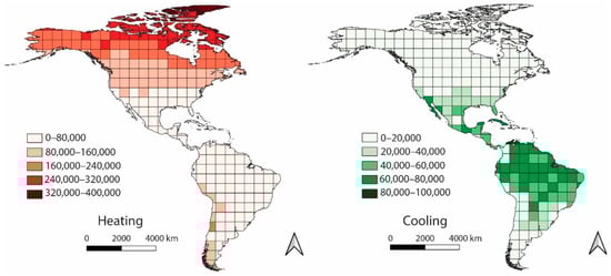
Figure 1.
Heating Degree Hours (HDH) and Cooling Degree Hours (CDH) of inlet air temperature for historical conditions. HDH and CDH were calculated by taking the difference from 18 °C if the inlet air temperature was lower and greater than 18 °C, respectively. Note the varying scales for HDH and CDH maps.
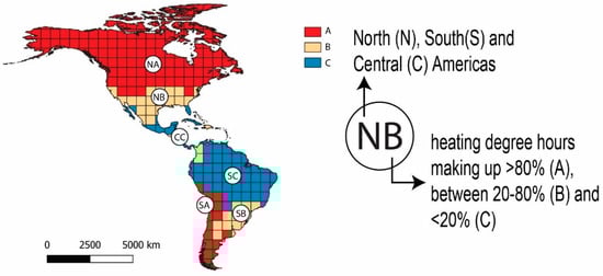
Figure 2.
Zones with heating degree hours making up >80% (A), between 20–80% (B), and <20% (C) of total annual heating and cooling degree hours describe different heating and cooling regimes in North (N), South (S), and Central (C) Americas.
A reduction of heating degree hours and increase in cooling degree hours are projected for the range of climate change scenarios projections. Higher latitudes showed the largest decrease in heating degree hours (Figure 3). Meanwhile, CC and SC regions showed a noticeable amplification of cooling needs (Figure 4). Regions experiencing noticeable changes in heating and cooling needs extended towards the equator and poles, respectively, for the later time interval (2061–2090) and more severe scenarios (RCP 4.5 and 8.5). It was therefore evident that changes to heating and cooling needs were concentrated to regions already dominated by those needs.
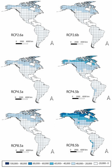
Figure 3.
Change in HDH (°C-hours) of the simulated inlet air temperature.
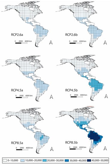
Figure 4.
Change in CDH (°C-hours) of the simulated inlet air temperature.
The magnitude of peak changes was greater for heating when compared to cooling. Cooling degree hour increases were typically in the range of 0–30,000 °C-hours, peaking around 50,000 °C-hours in the SC zone for the RCP8.5b scenario. On the other hand, heating degree hours at the inlet typically decreased by 0–40,000 °C, peaking at 100,000 °C for the RCP8.5b scenario. The difference in degree hour change magnitude was amplified further in the transitionary zones, where the heating degree hour change was roughly double that of the cooling degree hour change. These areas are temperate regions, such as the Northern United States and southern Canada, where heating and cooling needs and changes were more alike although heating needs did dominate. These results infer that projected climate change scenarios will likely increase cooling and decrease heating, the latter to a greater degree. Historically heating dominated areas therefore may observe a shift away from their dominant need. Historically cooling dominated areas may experience an amplification of their main air conditioning demand. These outcomes are in line with other studies on cooling energy demand under climate change scenarios—see for example [2].
3.2. Geo-Climatic Suitability for Projected RCP Scenarios
Using geo-climatic suitability criteria identified regions with a balance of heating and cooling needs as the most feasible regions for EAHE implication historically (Table 3, Figure 5). Heating geo-climatic suitability peaks at “High” for most of the NA with reductions to “Low” being observed in more polar regions. To the south of these “High” geo-climatic heating suitability regions, the feasibility decreases to “Medium” or “Low”. The SA region also historically observes “Medium” or “Low’ classifications. Notably tropical regions (CC and SC) observed a “Very Low” geo-climatic suitability attributable to the low heating needs in this region. In terms of cooling suitability regions with “Very High” characterization were observed in the mid-latitudes towards the subtropics in North America (NB) and in the mid-latitudes in South America to the east of the Andes (SB). “High” cooling suitability occurred around these locations, mostly to the north of the “Very High” suitability areas. “Low” and “Very Low” cooling suitability occurred in colder regions, particularly polar regions in North America and west of the Andes in South America. The distribution of geo-climatic suitability identified that regions with very low or high heating or cooling needs typically observed lower EAHE benefits. Climates with moderate heating and cooling, exhibiting a convergence of heating and cooling demand (SB and NB), had the highest geo-climatic suitability for cooling.
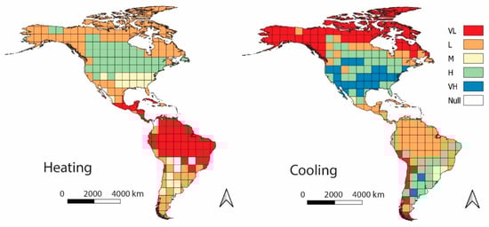
Figure 5.
Heat (left) and Cool (right) geo-climatic suitability categories for historical conditions.
Geo-climatic heating suitability decreased in subtropical regions and increased in colder climates (Figure 6). Subtropical regions (NB and SB) to the north and south of the tropical, “Very Low” heating suitability, zones displayed decreased heating usability. However, the changes are sporadic with the most noticeable change occurring in the RCP8.5b scenario. In this case, we can see the extension of “Low” and “Medium” suitability extending northward from the NB zone further into the NA zone. While the RCP8.5b expectedly showed the largest changes, there were less noticeable differences between the RCP2.6 and RCP4.5 scenarios as well as the 2021–2050 and 2061–2090 time periods for these RCPs. Ultimately, geo-climatic heating suitability changes for projected climate change scenarios were spatially limited and varied.
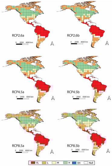
Figure 6.
Heating geo-climatic suitability categories for projected climate change scenarios.
Geo-climatic cooling suitability changes were more obvious, particularly in cooler regions (Figure 7). In South America, the higher suitability zones appeared to migrate towards the southern tip of the continent towards the eastern SA zone and SB. The increase in geo-climatic suitability was amplified for scenarios RCP4.5 and RCP8.5, with a larger contrast observed between 2021–2050 and 2061–2090 time periods as expected. A slight difference was seen in scenarios RCP4.5b and 8.5b in the southern most cells of South America (SA) increasing in suitability from historically “Low” classifications to “High” suitability. However, the majority of South America (SC), mainly the equatorial region, and central America (CC) remained “Low” or “High”. More noticeable differences were seen in North America, where there was a considerable extension of the “Very High” suitability zone from the mid-latitudes to polar regions into the Canadian Northern Territories (NA) for the most severe RCP8.5b. Similarly, RCP2.6 and RCP4.5 also had an increased suitability in the polar regions with evolution from “Very Low” and “Low” cooling suitability historically to “Low” and “High” suitability. For projected climate change scenarios, particularly the more severe cases, increased geo-climatic cooling suitability can occur in historically heating dominated regions.
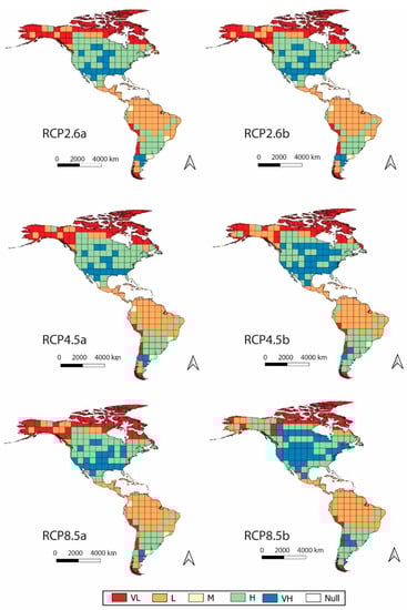
Figure 7.
Cooling geo-climatic suitability categories for projected climate change scenarios.
3.3. Change in Heating and Cooling Capacity
A distinct inverse spatial distribution of heating and cooling capacities, HDH% and CDH% (Equation (6)), was evident for historical conditions (Figure 8). Large values indicated that a greater proportion of the heating or cooling demand was being met by the system. It was readily identified that regions with low heating or cooling needs had the highest capacities. Tropical regions (SC and CC) recorded capacities >80% for heating. On the periphery of these regions, the heating capacity decreased until it reached a range of 0–20% throughout Canada and Alaska (NA) and the southern-western tip of South America (SA). Conversely, areas with low heating capacity corresponded to regions with peak cooling capacities of >80%. SB and NB regions displayed comparable heating and cooling capacities. Cooling and heating capacities ranged from ~40–70% and~ 20–50%, respectively, in the NB regions. The South American regions (SB) observed larger heating capacity, ~20–80%, when compared to the cooling capacity, ~10–60%. EAHE heating and cooling capacities therefore exhibit a noticeable pattern based on the latitudinal temperature gradients and the resultant space conditioning demand.
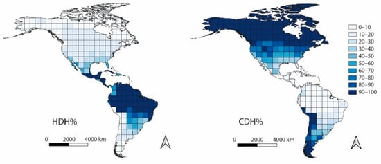
Figure 8.
Heating (HDH%, left) and cooling (CDH%, right) capacity of a hypothetical EAHEs.
Examining the results revealed a consistent pattern of capacity changes relative to characteristic heating and cooling regions. Heating capacity changes (ΔHDH%) had an increased potential in southern North America (NB) and south-eastern South America (SB) (Figure 9). Decreases to cooling capacity (ΔCDH%) occurred mostly in temperate regions in both North (southern NA and NB) and South America (SB and SA) (Figure 10). While heating capacity changes appeared greatest in temperate climates (SB and NB), changes to cooling capacity encroached onto cooler regions with the largest changes being observed along the boundary of NA and NB regions and within both SA and SB zones. Peak ΔHDH% changes of 40% for scenario RCP8.5b were determined in SB and only 30% in NB regions. Conversely, peak ΔCDH% values of −35–−20% were more widespread in North America compared to South America, although the largest magnitude change (−40–−35%) was observed along the SA and SB border. It should also be noted that these behaviors are best highlighted in the most severe scenarios (RCP4.5 and RCP8.5), particularly the later time period (2061–2090), with a much smaller contrast between regions and extent of areas affected for the other scenarios. This was especially the case for the RCP8.5b scenario in North America, where the upper geographic boundary for ~10% magnitude changes was expanded northwards. By contrasting the spatial distribution of peak ΔHDH% and ΔCDH%, it was evident that impacted areas were much more confined in South America, a reflection of the smaller areas of SB and SA relative to NA and NB zones. Outside these changes, large areas of North America (polar NA) and South America (SC and CC) observed menial changes of <10% in magnitude, for ΔHDH% and ΔCDH%, respectively, outside several grid units that behaved more so like B zones witnessing a particularly noticeable increase in heating capacity for RCP8.5b (>40%).
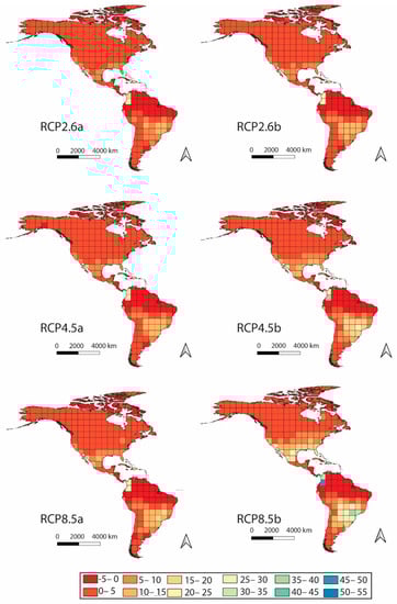
Figure 9.
ΔHDH% derived for six scenarios examined.
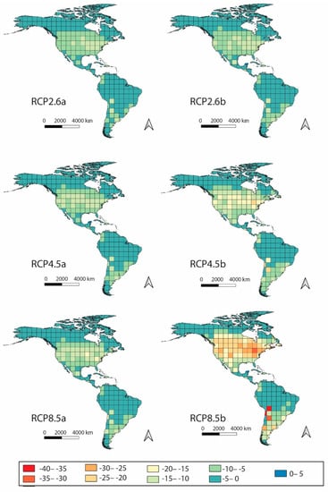
Figure 10.
ΔCDH% derived for six scenarios examined.
3.4. Variability in Capacity and Suitability
Variability of EAHE heating and cooling capacity was gauged by evaluating the EAHE potential using the first and third quarter percentile changes from the ensemble of future atmospheric parameters described by the GCM models. Contrasting the geo-climatic suitability classifications for the 25th, 75th, and median derived weather files highlighted the increased variability in later time periods (2061–2090) results (Table 4). In all cases, the scenarios for the 2021–2050 interval had a lower incidence of changing geo-climatic suitability when evaluated at the 25th and 75th percentiles relative to the classifications derived from the weather files generated using median changes in climate parameters. The largest number of changes was observed for the RCP4.5b, which had 17.2% of sites observing different results for heating. Meanwhile, for cooling, the highest variability occurred for the RCP8.5b scenario, which had 26.4% of sites affected. Expectedly, the highest variability in classifications was observed for RCP4.5b and RCP8.5b. Changes in classifications can be attributed to a combination of a large range of results from the GCMs and the discretization of the heating and cooling potential into the geo-climatic suitability categories, making regions sensitive to changes in values if they were near the category thresholds. The remaining scenarios typically showed different results for the upper and lower percentiles for roughly 10–15% of sites. This subset of sites demonstrated an uncertainty in the geo-climatic suitability for the projected scenarios. However, this also shows that 75–90% of locations converged on a single geo-climatic suitability classification for the entire interquartile range of model results.
Table 4.
Sum of class changes for 25th and 75th percentile weather files. There was a total of 546 comparisons made for the 273 locations.
In order to explore the spatial patterns for the variability in heating and cooling changes, the ΔHDH% and ΔCDH% range between the 25th and 75th percentile results were mapped (Equation (8), Figure 11 and Figure 12). Both parameters revealed similar patterns with the largest ΔHDH% and ΔCDH% ranges observed for the later time period scenarios (2061–2090) in agreement with the results of classification variability. In South America, the peak ranges were 20–25%. However, the ranges were greater towards the SA zones for ΔCDH% and SB for ΔHDH%. These correspond to the regions with the greatest ΔDH%. In North America, the magnitude of the ΔHDH% and ΔCDH% ranges were typically <10%, although there were some areas of heightened variability in the central-eastern portions of the NA region observed a noticeable range for ΔCDH%, peaking at ~20% for RCP8.5b. In terms of ΔHDH%, areas along the Gulf of Mexico observed ranges ~10%. Regions outside of these recognized areas typically exhibited a magnitude of 0–5% for the ΔHDH% and ΔCDH% ranges between 25th and 75th percentile results. These results demonstrated that calculated capacity changes using later time periods scenarios (b, 2061–2090), particularly for the southern portion of South America and North American mid-latitudes, were susceptible to increased variability.
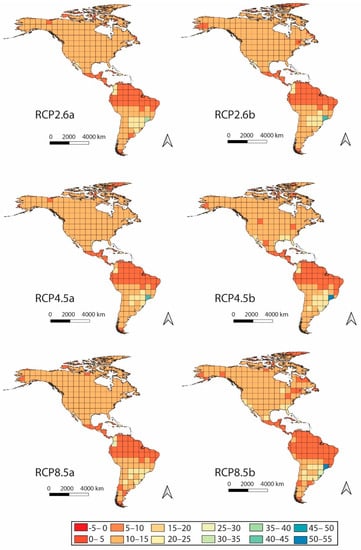
Figure 11.
HDH% range between the results for the weather files created with the 75th and 25th percentile change amongst the GCM models.
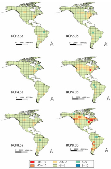
Figure 12.
CDH% range between the results for the weather files created with the 75th and 25th percentile change amongst the GCM models.
3.5. Seasonal Changes in Heating and Cooling Capacity
The estimation of heating (Figure 13) and cooling (Figure 14) capacity, and changes relative to historical conditions (Figure 15 and Figure 16) were also conducted on a seasonal basis for the most severe RCP8.5b scenario. If we consider capacity as the usability of the EAHE, then the seasonal analysis will inform how the applicability of the EAHE will change during different parts of the year. Seasonal capacity results demonstrate that for the projected conditions of RCP8.5b, NA and SA zones will be capable of addressing cooling needs, while SB, NB, SC, and CC zones have higher heating capacities. It should be noted that capacities converging to 100% are often the result of very low heating or cooling needs, for example in SC and CC zones for heating or Polar NA and SA zones for cooling. Nevertheless, the high capacity indicates that despite changing climatic conditions, the system will be able to address any heating or cooling needs if capacity is near 100%. There are also seasonal variations in the capacity, which are most obvious for NA, SA, NB, and SB zones. From September–February, the NA zones see a marked increase in capacity to ~30–40%. While not as great, a similar increase is observable in SA from March–August. Both of these results demonstrate that in heating dominated climates, the capacity of the EAHE is greatest when heating demand is greatest. For cooling, in the NA/NB and SA/SB zones the lowest capacities are observed mostly during September–November and March–May, respectively. While in these periods capacity lowers to <30% for the warmer segments within these zones (NB or SB), large swaths of the NA and SA areas persist with capacities >40%. During peak cooling seasons, NA and SA zones see more widespread lower capacities (~40%). While this coincides with increased cooling demand, the magnitude of the cooling capacity (CDH%) is still large relative to heating capacity (HDH%).
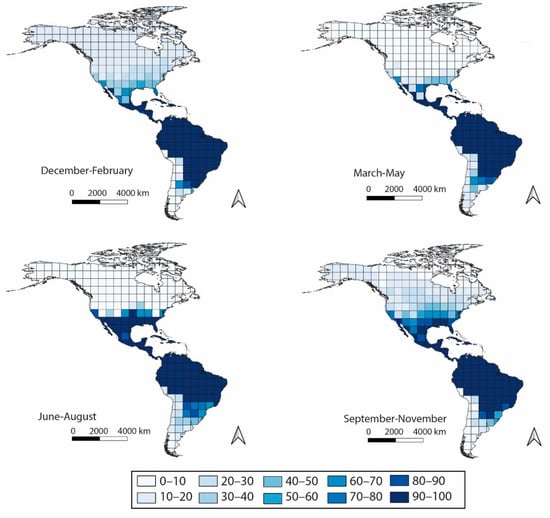
Figure 13.
HDH% for the RCP8.5 scenario for the years 2061–2090 on a seasonal basis.
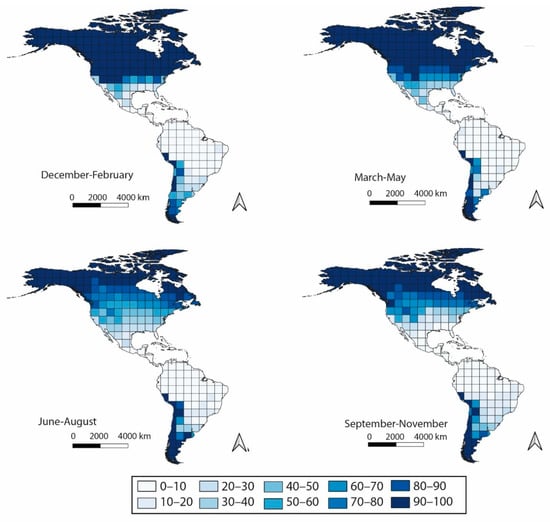
Figure 14.
CDH% for the RCP8.5 scenario for the years 2061–2090 on a seasonal basis.
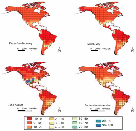
Figure 15.
ΔHDH% calculated on a seasonal basis.
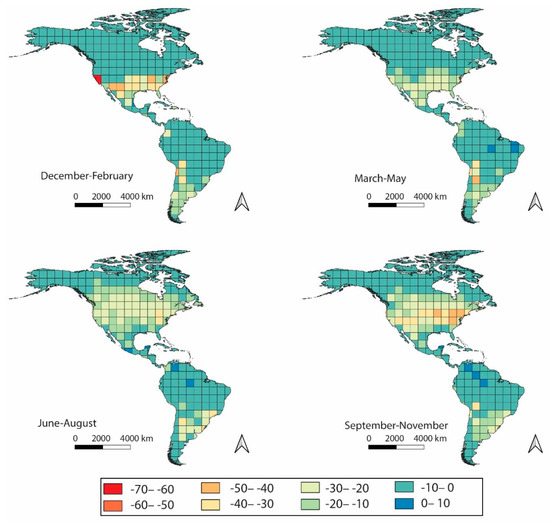
Figure 16.
ΔCDH% calculated on a seasonal basis.
In terms of magnitude, it is obvious that the largest changes in heating capacity changes are observed during the summer for the NB zone where capacity increases (Figure 15). This is likely the result of warming temperatures eliminating heating needs from June–August, where historical needs are already low. A similar effect can be seen during the September–November season as well. Therefore, the most drastic changes in heating for North America are occurring when heating is demand is the lowest. On the other hand, in the SB zone during June–November, the changes are the greatest. During this period, heating needs are expected to be greatest. As a result, in contrast to North America, zones experiencing changes in South America have the largest magnitude changes during heat demanding seasons. SC and CC regions observed minimal discernable seasonal variations.
In terms of cooling, North America revealed a susceptibility to rising cooling needs (Figure 16). North America had the largest extent of noticeable CDH% reductions during the cooling season from June–August, and to a lesser degree September–November, when needs were greatest. These were mainly affecting the lower portions of NA at the NB boundary. During the December–May period in North America, the reduction in CDH crept into the NB zone with high magnitudes of change (>−40%). During this period, in South America, the SA zone saw some of the greatest changes. Meanwhile, the CDH% reductions were confined more to the SB zone from June–August. These results demonstrate that during the cooling seasons (June–September in the Northern Hemisphere and December–May in the Southern Hemisphere) the cooler NA and SA zones experience more obvious reductions in cooling capacity, whereas the more moderate climates, SB and NB, observed more changes in the off-cooling seasons. Again, like heating, there were few identifiable trends in the SC and CC zones on a seasonal basis. This can be attributed to the reduced seasonality in these zones.
4. Discussion
4.1. Changes to EAHE Potential and Suitability
Differing trends between the geo-climatic suitability and ΔDH% provide a qualitative understanding of EAHE usability under projected climate change scenarios. Positive heating capacity changes identified an improvement in EAHE heating expectedly due to the reduction in demand for projected climate change scenarios. In cooler regions where significant heating needs persist despite warmer temperatures, the increased heating capacity was still valuable. Conversely, climates requiring little heating observed a reduction in suitability in response to diminishing heating demand. It can be understood that the increasing ΔHDH% indicated an enhanced ability to consistently provide heating when needed, while the geo-climatic suitability characterization identified if that heating was valuable for the location. Rightfully, EAHE systems are likely not feasible solely for heating in subtropical climates due to their weakened utility.
Decreased CDH% in conjunction with persistent and expanding “High” or “Very High” cooling geo-climatic suitability demonstrate that EAHEs can continue to be feasible in mid-latitude, temperate zones in both North and South America. For more severe scenarios (RCP8.5b and 4.5b), regions with historically lower cooling needs also showed increases in CDH. In these regions, despite the increase in cooling needs, geo-climatic suitability was maintained or improved. The cooling capacities in these regions were reduced due to increased cooling needs. However, the usability of the systems was conserved, since it was able to still provide a significant portion of cooling while the value of the cooling was enhanced due to the greater cooling demand. Increasing cooling needs in historically cooling dominated climates on the other hand did not receive any benefits from increased needs, since the systems were already finding it difficult to meet the capacity. Furthermore, historically heating dominated areas, particularly in the higher latitudes, witnessed an increase in a geo-climatic suitability, while some remained at a “Low” or “Very Low” suitability classification. The areas with increased suitability can be attributed to a significant enough increase in cooling demand amplifying the value of the cooling capacity at these sites, while the unfavorable sites still did not have enough cooling need to justify EAHE use despite high cooling capacities. The response of EAHE cooling feasibility therefore varied among regions based on cooling demand for projected climate change scenarios. Evaluating both capacity and geo-climatic suitability realized that temperate regions in North (southern NA) and South America (SA and SB) were most feasible for EAHE implementation when considering the effect of projected climate change conditions. In these regions, the highest geo-climatic suitability was observed for both heating and cooling. It is also of interest that new frontiers for EAHE implementation may be generated by climate changes in historically unfavorable regions. North American polar regions that combine high cooling capacity with increasing cooling needs are expected to produce improvements in geo-climatic cooling suitability, while reductions in heating needs will help alleviate the consequences of low heating capacity. Conversely, historically unfavorable central America (CC) and the northern portion of South America (SC) are expected to remain ineffective at providing either heating or cooling, illustrated by consistent “Low” and “Very Low” classes. This can be attributed to high, and increasing, cooling demand in conjunction with a reduced capacity to meet these needs. Ultimately, the impact of climate changes on EAHE suitability can be separated regionally due to the relationship between climate and heating or cooling demands, in addition to system function.
Examining the seasonal heating and cooling capacities for the RCP8.5b scenario further highlights that seasonal cooling capacity reductions are most apparent in temperate regions, particularly during peak cooling demand periods for cooler zones (NA and SA). The capacities for this most severe scenario will remain high for cooling in cold regions and heating in warm regions. The transitionary temperate regions (NA/NB and SB/SA) will see variations both seasonally and temporally, relative to baseline historical conditions. Heating improvements will occur in seasons with lower heating needs. On the other hand, cooling reductions will be most obvious during cooling dominant periods in these regions, as cooling needs intensify and extend into the following season. For example, in temperate NA, we see the largest ΔCDH% from September–November, likely a result of increased cooling needs during this period with little capacity following the ground warming from June–August in the northern hemisphere. This illustrates that the ability of EAHEs to meet cooling needs will be hampered most during periods with enhancing cooling needs. Therefore, changing climatic conditions will degrade the cooling potential of EAHEs when they are needed most. However, the high suitability regions (temperate NA and SA/SB) identified from the geo-climatic suitability analysis still maintain useable capacity (>20%) during peak heating and cooling periods. Stakeholders should be aware of the reduction in cooling capacity during peak cooling seasons when compared to historical annual results (Figure 8) to ensure that EAHE cooling will not underperform on a seasonal basis due to seasonal variations.
4.2. Variability in Heating and Cooling Capacity Changes
The analyses are subject to uncertainty due to the use of an ensemble of GCM outputs. By calculating the results for 75th and 25th percentile changes in addition to the median, the variability of the outputs was gauged. Comparing the range of ΔHDH% and ΔCDH%, it was evident that the range in these values for the 75th and 25th results was typically larger for scenarios with greater predicted changes in capacity. This was particularly noticeable for the higher RCP and later time period scenarios, RCP4.5b and 8.5b. Typically, the range in capacity changes was between 0–5%, and often <10%. This range, particularly for cooling capacity changes, was significantly less than the magnitude of changes estimated. Pockets of >10% ranges in cooling capacity were evident in temperate North America (southern NA). This behavior became particularly prominent for the cooling capacity in scenario RCP8.5b. The areas affected were coincident with the areas observing the largest magnitude ΔCDH%. A more spatially distinct region of high ΔHDH% and ΔCDH% variability coincident with large changes in the SB region was recognized for the more severe scenarios. These observations agree with the expected divergence of GCM outputs for later time periods and higher RCPs, where the magnitude of changes increases. For areas with larger degrees of variability, such as the southern portion of South America and mid-latitude regions in North America (for cooling), a higher resolution of climate models is suggested to better constrain the changes. Ultimately, the variability observed in the changes to capacity was much lower than the changes predicted, providing confidence in the estimated trend in increasing and decreasing heating and cooling capacities.
5. Conclusions
A climate driven approach to estimate EAHE suitability for projected climate change scenarios was used across the Americas. The findings showed:
- EAHE feasibility in cooling dominated regions (CC and SC) is expected to remain low with increasing cooling needs and insufficient capacity.
- Reduction of heating demand and growth of cooling needs will improve the feasibility of EAHEs in extremely cold climates (NA and SA).
- The value of cooling in temperate regions (NA, NB, SB and SA) will improve or be maintained, although capacity will be hampered, while heating suitability will remain relatively consistent
- Variability in the estimated change in EAHE potential was greatest for the most severe RCP scenarios (RCP4.5 and RCP8.5) and latter time periods, peaking at ~26%, with 10–26% of sites observing variable geo-climatic suitability classifications within the interquartile range of GCM model results.
- Seasonal analysis of heating and cooling capacity changes highlighted cooler regions (NA and SA) will experience larger changes during seasons with higher cooling demands.
While the results paint a noticeable response by EAHE capacity and suitability to climate changes, they cannot be examined without consideration for the underlying limitations of the approach used. Besides the uncertainty of GCM outputs already discussed, the climate-based approach is limited by the parameterization of the EAHE system. Notably, the system does not include an interaction between the system and the surrounding subsurface; instead, the undisturbed ground temperature at depth is used. As a result, the potential of EAHE systems may be overestimated due to the absence of “soil derating”. The efficiency of the system is also set as a constant throughout the entire annual period by maintaining constant system dimensions, operational control (air flow) and soil conditions. However, the efficiency can vary with the thermal characteristics of the surrounding soil and operational control of the system. Particularly, the effects of soil freezing are not encompassed in the analysis. Temporal heterogeneities in soil properties, such as those brought on by soil freezing during cold seasons, can hypothetically alter the EAHE capacity [67]. In addition to temporal heterogeneities of soil thermal properties at a site, soil types and properties can vary significantly spatially. Sandy soil was selected to avoid overestimating EAHE potential, as it describes a lower system efficiency relative to dry or humid clay conditions [39]. As a result, stakeholders should establish soil properties once the conditions of the considered sites can be better estimated beyond the pre-design stage. The approach also does not include the impact of climate changes on the building being supplied by the EAHE. Future work will endeavor to include the hypothetical building’s response to climate change to evaluate the combined impact of projected climate change scenarios on EAHE heating and cooling for building use. To supplement this analysis, future work could also use historical weather and EAHE performance data to forecast their future performance. Contrasting the outcomes from this present study with forecasts of actual observed data would hypothetically reveal the omission of any significant factors in the approach used. Therefore, while these simplifications allow for a rapid assessment of EAHE potential necessary for examining a multitude of projected climate change scenarios and many locations, the limitations need to be considered when exploring the approach’s outputs. Nevertheless, the geo-climatic suitability’s of EAHEs show a varying response to changing climatic conditions across the Americas that should be considered by designers and policy makers looking to implement these systems. Based on potential future changes to EAHE potential, cooler temperate regions in the Americas should advocate for EAHE use due to high continued suitability for both heating and cooling despite projected climate changes.
Author Contributions
Conceptualization: A.Z. and W.A.G.; methodology: A.Z., W.A.G., and G.C.; investigation: A.Z.; writing—original draft preparation: A.Z. and G.C.; writing—review and editing: W.A.G. and G.C.; visualization: A.Z.; supervision: W.A.G.; funding acquisition: W.A.G. All authors have read and agreed to the published version of the manuscript.
Funding
This work was supported by the Natural Sciences and Engineering Research Council of Canada (NSERC), Discovery Grant [RGPIN-2018-06801].
Acknowledgments
The authors thank and acknowledge the World Climate Research Programme’s Working Group on Coupled Modelling, who are responsible for the CMIP5 project. The authors would also like to thank the U.S. Department of Energy’s Program for Climate Model Diagnosis and Intercomparison, which provides coordinating support and led the generation of software infrastructure, in partnership with the Global Organization for Earth System Science Portals, which allowed a means for the download and use of the CMIP5 data. We are also thankful to the modelling groups who have made their model output data available. Table 1 lists the working groups and their respective models used in this work. We would like to thank the reviewers for their thoughts and comments on this work.
Conflicts of Interest
The authors declare no conflict of interest.
References
- European Parliament. Directive 2018/844/EU of the European Parliament and of the Council of 30 May 2018 amending Directive 2010/31/EU on the energy performance of buildings and Directive 2012/27/EU on energy efficiency. Off. J. Eur. Union 2018, 61, 43–74. [Google Scholar]
- Santamouris, M. (Ed.) Cooling Energy Solutions for Buildings and Cities; World Scientific: Singapore, 2019. [Google Scholar]
- Santamouris, M. (Ed.) Advances in Passive Cooling; Earthscan: London, UK, 2007. [Google Scholar]
- Heiselberg, P. (Ed.) Ventilative Cooling Design Guide; IEA EBC ANNEX 62; Aalborg University: Aalborg, Denmark, 2018. [Google Scholar]
- Chiesa, G. Optimisation of envelope insulation levels and resilience to climate changes. In Sustainable Technologies for the Enhancement of the Natural Landscape and of the Built Environment; De Joanna, P., Passaro, A., Eds.; LucianoEditore: Naples, Italy, 2019; pp. 339–372. [Google Scholar]
- Kolokotroni, M.; Heiselberg, P. (Eds.) Ventilative Cooling State-of-the-Art Review; IEA EBC ANNEX 62; Aalborg University: Aalborg, Denmark, 2015. [Google Scholar]
- Carlucci, S.; Pagliano, L.; Sangalli, A. Statistical analysis of the ranking capability of long-term thermal discomfort indices and their adoption in optimization processes to support building design. Build. Environ. 2014, 75, 114–131. [Google Scholar] [CrossRef]
- Givoni, B. Passive and Low Energy Cooling of Buildings; Van Nostrand Reinhold: New York, NY, USA, 1994. [Google Scholar]
- Cook, J. (Ed.) Passive Cooling; MIT Press: Boston, MA, USA, 2000. [Google Scholar]
- Grosso, M. Il Raffrescamento Passivo Degli Edifici in Zone a Clima Temperato, 4th ed.; Maggioli: Santarcangelo di Romagna, Italy, 2017. [Google Scholar]
- Pfafferott, J. Evaluation of earth-to-air heat exchangers with a standardised method to calculate energy efficiency. Energy Build. 2003, 35, 971–983. [Google Scholar] [CrossRef]
- Peretti, C.; Zarrella, A.; De Carli, M.; Zecchin, R. The design and environmental evaluation of earth-to-air heat exchangers (EAHE). A literature review. Renew. Sustain. Energy Rev. 2013, 28, 107–116. [Google Scholar] [CrossRef]
- Khabbaz, M.; Benhamou, B.; Limam, K.; Hamdi, H.; Hollmuller, P.; Bennouna, A. Experimental and numerical study of an earth-to-air heat exchanger for air cooling in a residential building in hot semi-arid climate. Energy Build. 2016, 125, 109–121. [Google Scholar] [CrossRef]
- Hsu, C.-Y.; Chiang, Y.-C.; Chien, Z.-J.; Chen, S.-L. Investigation on performance of building-integrated earth-air heat exchanger. Energy Build. 2018, 169, 444–452. [Google Scholar] [CrossRef]
- Kaushal, M. Geothermal cooling/heating using ground heat exchanger for various experimental and analytical studies: Comprehensive review. Energy Build. 2017, 139, 634–652. [Google Scholar] [CrossRef]
- Su, H.; Liu, X.-B.; Ji, L.; Mu, J.-Y. A numerical model of a deeply buried air–earth–tunnel heat exchanger. Energy Build. 2012, 48, 233–239. [Google Scholar] [CrossRef]
- Cucumo, M.; Cucumo, S.; Montoro, L.; Vulcano, A. A one-dimensional transient analytical model for earth-to-air heat exchangers, taking into account condensation phenomena and thermal perturbation from the upper free surface as well as around the buried pipes. Int. J. Heat Mass Transf. 2008, 51, 506–516. [Google Scholar] [CrossRef]
- Kumar, R.; Kaushik, S.; Garg, S. Heating and cooling potential of an earth-to-air heat exchanger using artificial neural network. Renew. Energy 2006, 31, 1139–1155. [Google Scholar] [CrossRef]
- Benkert, S.; Heidt, F.D.; Schöler, D. Calculation Tool for earth heat exchangers GAEA. In Proceedings of the Building Simulation 1997, 5th International IBPSA Conference, Prague, Czech Republic, 8–10 September 1997; pp. 9–16. [Google Scholar]
- Raimondo, L. Potenziale di raffrescamento da scambiatore geotermico ad aria. In Il Raffrescamento Passivo Degli Edifici, 2nd ed.; Grosso, M., Ed.; Maggioli: Santarcangelo di Romagna, Italy, 2008; pp. 441–454. [Google Scholar]
- Misra, R.; Bansal, V.; Das Agrawal, G.; Mathur, J.; Aseri, T. Transient analysis based determination of derating factor for earth air tunnel heat exchanger in summer. Energy Build. 2013, 58, 103–110. [Google Scholar] [CrossRef]
- Bansal, V.; Misra, R.; Das Agarwal, G.; Mathur, J. ‘Derating Factor’ new concept for evaluating thermal performance of earth air tunnel heat exchanger: A transient CFD analysis. Appl. Energy 2013, 102, 418–426. [Google Scholar] [CrossRef]
- Grosso, M.; Raimondo, L. Horizontal air-to-Earth heat exchangers in Northern Italy—testing, design and monitoring. Int. J. Vent. 2008, 7, 1–10. [Google Scholar] [CrossRef]
- Grosso, M.; Chiesa, G. Horizontal Earth-to-air heat exchanger in Imola, Italy. A 30-month- long monitoring campaign. Energy Procedia 2015, 78, 73–78. [Google Scholar] [CrossRef]
- Chiesa, G.; Simonetti, M.; Grosso, M. A 3-field earth-heat-exchange system for a school building in Imola, Italy: Monitoring results. Renew. Energy 2014, 62, 563–570. [Google Scholar] [CrossRef]
- Lee, K.H.; Strand, R.K. The cooling and heating potential of an earth tube system in buildings. Energy Build. 2008, 40, 486–494. [Google Scholar] [CrossRef]
- Xamán, J.; Hernández-López, I.; Alvarado-Juárez, R.; Hernández-Pérez, I.; Álvarez, G.; Chávez, Y. Pseudo transient numerical study of an earth-to-air heat exchanger for different climates of México. Energy Build. 2015, 99, 273–283. [Google Scholar] [CrossRef]
- Bansal, V.; Misra, R.; Das Agrawal, G.; Mathur, J. Performance analysis of earth–pipe–air heat exchanger for summer cooling. Energy Build. 2010, 42, 645–648. [Google Scholar] [CrossRef]
- D’Agostino, D.; Esposito, F.; Greco, A.; Masselli, C.; Minichiello, F. The energy performances of a ground-to-air heat exchanger: A comparison among Köppen climatic areas. Energies 2020, 13, 2895. [Google Scholar] [CrossRef]
- Zajch, A.M.; Gough, W.A. Employing the Climate Based Approach for Determining Earth-Air Heat Exchanger Feasibility in the Context of Canadian Climates. In Proceedings of the Grand Renewable Energy 2018 International Conference and Exhibition, Yokohama, Japan, 17–22 June 2018. [Google Scholar]
- Zhang, C.; Wang, J.; Li, L.; Wang, F.; Gang, W. Utilization of earth-to-air heat exchanger to pre-cool/heat ventilation air and its annual energy performance evaluation: A case study. Sustainability 2020, 12, 8330. [Google Scholar] [CrossRef]
- Rodríguez-Vázquez, M.; Xamán, J.; Chávez, Y.; Hernández-Pérez, I.; Simá, E. Thermal potential of a geothermal earth-to-air heat exchanger in six climatic conditions of México. Mech. Ind. 2020, 21, 308. [Google Scholar] [CrossRef]
- Ramírez-Dávila, L.; Xamán, J.; Arce, J.; Álvarez, G.; Hernández-Pérez, I. Numerical study of earth-to-air heat exchanger for three different climates. Energy Build. 2014, 76, 238–248. [Google Scholar] [CrossRef]
- Fazlikhani, F.; Goudarzi, H.; Solgi, E. Numerical analysis of the efficiency of earth to air heat exchange systems in cold and hot-arid climates. Energy Convers. Manag. 2017, 148, 78–89. [Google Scholar] [CrossRef]
- D’Agostino, D.; Greco, A.; Masselli, C.; Minichiello, F. The employment of an earth-to-air heat exchanger as pre-treating unit of an air conditioning system for energy saving: A comparison among different worldwide climatic zones. Energy Build. 2020, 229, 110517. [Google Scholar] [CrossRef] [PubMed]
- Chiesa, G.; Zajch, A. Geo-climatic applicability of earth-to-air heat exchangers in North America. Energy Build. 2019, 202, 109332. [Google Scholar] [CrossRef]
- Alves, A.B.M.; Schmid, A.L. Cooling and heating potential of underground soil according to depth and soil surface treatment in the Brazilian climatic regions. Energy Build. 2015, 90, 41–50. [Google Scholar] [CrossRef]
- Chiesa, G. Climate-potential of earth-to-air heat exchangers. Energy Procedia 2017, 122, 517–522. [Google Scholar] [CrossRef]
- Chiesa, G. EAHX—Earth-to-air heat exchanger: Simplified method and KPI for early building design phases. Build. Environ. 2018, 144, 142–158. [Google Scholar] [CrossRef]
- Shen, P.; Lukes, J.R. Impact of global warming on performance of ground source heat pumps in US climate zones. Energy Convers. Manag. 2015, 101, 632–643. [Google Scholar] [CrossRef]
- Zhu, K.; Blum, P.; Ferguson, G.; Balke, K.-D.; Bayer, P. The geothermal potential of urban heat islands. Environ. Res. Lett. 2010, 5, 5. [Google Scholar] [CrossRef]
- Allen, A.; Milenic, D.; Sikora, P. Shallow gravel aquifers and the urban ‘heat island’ effect: A source of low enthalpy geothermal energy. Geothermics 2003, 32, 569–578. [Google Scholar] [CrossRef]
- Luo, Z.; Asproudi, C. Subsurface urban heat island and its effects on horizontal ground-source heat pump potential under climate change. Appl. Therm. Eng. 2015, 90, 530–537. [Google Scholar] [CrossRef]
- Zajch, A.; Gough, W.; Chiesa, G. Earth–Air Heat Exchanger Potential Under Future Climate Change Scenarios in Nine North American Cities. In Sustainability in Energy and Buildings. Smart Innovation, Systems and Technologies; Littlewood, J., Howlett, R., Capozzoli, A., Jain, L., Eds.; Springer: Singapore, 2020; Volume 163. [Google Scholar] [CrossRef]
- Chiesa, G. Including EAHX (earth-to-air heat exchanger) in early-design phases considering local bioclimatic potential and specific technological requirements. IOP Conf. Series: Mater. Sci. Eng. 2019, 609, 032040. [Google Scholar] [CrossRef]
- QGIS.org. QGIS Geographic Information System, Version 3.14.15; Open Source Geospatial Foundation Project. 2019. Available online: http://qgis.org (accessed on 4 June 2020).
- ArcGIS. Available online: https://www.arcgis.com/home/item.html?id=5cf4f223c4a642eb9aa7ae1216a04372 (accessed on 6 September 2019).
- Meteotest. Meteonorm Software, v7.1.11; Meteotest: Bern, Switzerland, 2015. [Google Scholar]
- Meteotest. Meteonorm Handbook Part I; Meteotest: Bern, Switzerland, 2017. [Google Scholar]
- ESGF CMIP5 Data Search. Available online: https://esgf-node.llnl.gov/search/cmip5/ (accessed on 13 December 2018).
- Taylor, K.E.; Balaji, V.; Hankin, S.; Juckes, M.; Lawrence, B.; Pascoe, S. CMIP5 Data Reference Syntax (DRS) and Controlled Vocabularies. 2012. Available online: https://www.medcordex.eu/cmip5_data_reference_syntax.pdf (accessed on 3 December 2020).
- Van Vuuren, D.; Edmonds, J.; Kainuma, M.; Riahi, K.; Thomson, A.; Hibbard, K.; Hurtt, G.C.; Kram, T.; Krey, V.; Lamarque, J.-F.; et al. The representative concentration pathways: An overview. Clim. Chang. 2011, 109, 5–31. [Google Scholar] [CrossRef]
- R Core Team. R: A Language and Environment for Statistical Computing; R Foundation for Statistical Computing: Vienna, Austria, 2018. [Google Scholar]
- Pierce, D. ncdf4: Interface to Unidata netCDF (Version 4 or Earlier) Format Data Files. R Package Version 1.16. 2017. Available online: https://CRAN.R-project.org/package=ncdf4 (accessed on 3 December 2018).
- Wickham, H.; François, R.; Henry, L.; Müller, K. dplyr: A Grammar of Data Manipulation. R Package version 0.7.8. 2018. Available online: https://CRAN-R-project.org/package=dplyr (accessed on 28 November 2018).
- Wickham, H.; Hester, J.; Francois, R. readr: Read Rectangular Text Data. R Package Version 1.3.1. 2018. Available online: https://CRAN.R-project.org/package=readr (accessed on 1 May 2020).
- Wickham, H. stringr: Simple, Consistent Wrappers for Common String Operations. R package Version 1.3.1. 2018. Available online: https://CRAN.R-project.org/package=stringr (accessed on 28 November 2018).
- Schulzweida, U. CDO User Guide (Version 1.9.8). 2019. Available online: http://doi.org/10.5281/zenodo.3539275 (accessed on 28 December 2019).
- Belcher, S.; Hacker, J.; Powell, D. Constructing design weather data for future climates. Build. Serv. Eng. Res. Technol. 2005, 26, 49–61. [Google Scholar] [CrossRef]
- Benkert, S.; Heidt, F.D. Designing Earth Heat Exchangers—Validation of Software GAEA. In The energy for the 21st Century, World renewable Energy Congress VI; Elsevier: Brighton, UK, 2000; Chapter 380; pp. 1818–1821. [Google Scholar] [CrossRef]
- Ali, S.; Muhammad, N.; Amin, A.; Sohaib, M.; Basit, A.; Ahmad, T. Parametric Optimization of Earth to Air Heat Exchanger Using Response Surface Method. Sustainability 2019, 11, 3186. [Google Scholar] [CrossRef]
- Kopecky, P. Hygro-thermal performance of earth-to-air heat exchangers. Numerical model, analytical and experimental validation, measurements in-situ, design. Ph.D. Thesis, Czech Technical University, Prague, Czech Republic, 2008. [Google Scholar]
- Lab, K. Regional Analysis of Ground and above-Ground Climate; Oak Ridge National Laboratory: Springfield, VA, USA, 1981. [Google Scholar]
- U.S. Department of Energy. Engineering Reference (EnergyPlusTM Version 8.7.0 Documentation). Available online: https://energyplus.net/sites/all/modules/custom/nrel_custom/pdfs/pdfs_v8.7.0/EngineeringReference.pdf (accessed on 17 June 2020).
- U.S. Department of Energy. Auxiliary Programs (EnergyPlus—Version 8.7.0 Documentation). Available online: https://bigladdersoftware.com/epx/docs/8-7/auxiliary-programs/index.html (accessed on 17 June 2020).
- Government of Canada. Glossary. 2018. Available online: http://climate.weather.gc.ca/glossary_e.html (accessed on 24 September 2018).
- Zajch, A.; Gough, W.A. Seasonal sensitivity to atmospheric and ground surface temperature changes of an open earth-air heat exchanger in Canadian climate. Geothermics 2021, 89, 101914. [Google Scholar] [CrossRef]
Publisher’s Note: MDPI stays neutral with regard to jurisdictional claims in published maps and institutional affiliations. |
© 2020 by the authors. Licensee MDPI, Basel, Switzerland. This article is an open access article distributed under the terms and conditions of the Creative Commons Attribution (CC BY) license (http://creativecommons.org/licenses/by/4.0/).