Article

Incorporating Reservoir Greenhouse Gas Emissions into Carbon Footprint of Sugar Produced from Irrigated Sugarcane in Northeastern Nigeria

by
Taitiya Kenneth Yuguda
1,*,
Yi Li
1,
Bobby Shekarau Luka
2 and
Goziya William Dzarma
3
1
Key Laboratory of Integrated Regulation and Resource Development on Shallow Lakes, Ministry of Education, College of Environment, Hohai University, Nanjing 210098, China
2
Department of Agricultural Engineering, Federal University Wukari, 200 Katsina-Ala Road, Wukari 234, Nigeria
3
Department of Chemical Engineering, Michael Okpara University of Agriculture, Umuahia P.M.B. 7267, Nigeria
*
Author to whom correspondence should be addressed.
Sustainability 2020, 12(24), 10380; https://doi.org/10.3390/su122410380
Submission received: 23 November 2020 / Revised: 4 December 2020 / Accepted: 9 December 2020 / Published: 11 December 2020
(This article belongs to the Section Air, Climate Change and Sustainability)

Abstract

:
Greenhouse gas (GHG) emissions from reservoirs are responsible for at most 2% of the overall warming effects of human activities. This study aimed at incorporating the GHG emissions of a reservoir (with irrigation/sugar production as its primary purpose), into the carbon footprint of sugar produced from irrigated sugarcane. This study adopts a life-cycle assessment (LCA) approach and encompasses the cradle-to-gate aspect of the international organization of standardization ISO 14040 guidelines. Results show that total carbon footprint of refined sugar could be as high as 5.71 kg CO2-eq/kg sugar, over its entire life cycle, depending on the priority of purposes allocated to a reservoir and sugarcane productivity. Findings also reveal that the dammed river contributes the most to GHG emissions 5.04 kg CO2-eq/kg sugar, followed by the agricultural stage 0.430 kg CO2-eq/kg sugar, the sugar factory 0.227 kg CO2-eq/kg sugar, and lastly the transportation stage 0.065 kg CO2-eq/kg sugar. The sensitivity analysis shows that carbon footprint CF of sugar production is largely influenced by the rate of biomass decomposition in the impounded reservoir over time, followed by the reservoir drawdown due to seasonal climatic fluctuations. Significant amounts of GHG emissions are correlated with the impoundment of reservoirs for water resource development projects, which may account for up to 80% of total GHG emissions to the reservoir’s primary purpose. Sugar production expansion, coupled with allocating more functions to a reservoir, significantly influences the CF of sugar per service purpose. This study is an indicator for policymakers to comprehend and make plans for the growing tradeoffs amongst key functions of reservoirs.

Graphical Abstract

1. Introduction

The most significant driver of observed climate change since the mid-20th century is greenhouse gases (GHGs) emissions from human activities [1]. GHGs are naturally occurring and are essential to human survival and also to the survival of millions of other living organisms. However, over one and a half centuries of industrialization, deforestation, and large-scale agriculture have increased the amount of GHGs in the atmosphere to record levels unseen in three million years [2]. Growth in populations, economies, and life quality will continue to influence the cumulative level of GHGs emissions [3]. The carbon footprint, the most rapidly growing indicator, is approximately 60% of humanity’s relative ecological footprint and has risen 11-fold since 1961 [4].
Human-made reservoirs around the world, especially in the tropics, are significant sources of global GHG pollution, fueled by the decomposition of organic matter from the vegetation and soils flooded during impoundment [5]. GHG emissions from reservoirs created to irrigate crops, produce hydropower, achieve water security, or provide flood protection may be significant. They should be taken into account in the development and construction of new dam projects. Globally, quite many studies in recent decades have reported estimates of the total contribution of reservoir GHGs to global emissions Figure 1. The very first estimates in 2002 of global reservoir emissions reported quite a significant volume (7%) of global GHG emissions across all sources [6]. The standard approach employed by these authors involves making observations from the average specific emissions and deduce them to a global reservoir surface in standard units such as mg/m2 and year. While uncertainties are inevitable in these estimates, especially considering the reservoir’s total area, inadequate data and seasonal variations in the area of the reservoir render estimating the total area of freshwater lakes and reservoirs cumbersome. However, Downing JA, et al. [7] estimated that lakes occupy a global area of 3.7–4.2 million km2. A comprehensive study by Ivan Lima and colleagues, at the National Space Research Institute (INPE) of Brazil, utilized modeling techniques, bootstrap resampling, and data issued by the International Commission on Large Dams (ICOLD). Results show that large dams in the world emit 104 million metric tons of methane every year from reservoir surfaces, turbines, spillways, and downstream rivers [8]. The emergence of Global Reservoir and Dam (GRanD) Database developed by the Global Water System Project [9] was a turning point for reservoirs. The GRanD is a global data repository comprising several variables on 6862 reservoirs globally, with a total capacity of over 0.1 km3. It includes almost all of the world’s dammed reservoirs [10].
Previous estimates by Reference [11] depended nearly entirely on CO2, calculated from temperature, alkalinity, and pH using PHREEQC version 2. They reported values that are 4% higher than the 2100 Tg C obtained by Raymond PA et al. [12], who applied numerical models for estimating total annual emissions from streams, rivers, lakes, and reservoirs. The findings from Reference [13] suggest that reservoir emissions are just a fraction (<l%) of overall emissions from freshwater sources. Based on the report by UNESCO/IHA, the G-res tool was used recently to estimate emissions from a global database of single-purpose hydropower projects. Validation of installed capacity and energy production demonstrated linkage to the reservoir specific purpose [14]. Scherer L, & Pfister S. [15] adopted generalized linear models (GLMs) models, and findings indicate that hydropower carbon footprint was much more than predicted, with a global average of 173 kg CO2/MWh and 2.95 kg CH4/MWh emitted respectively. However, the cumulative average carbon footprint in terms of GWP100 was approximately 273 kg CO2-eq/MWh. Considering the global significance of natural systems, it is anticipated that footprints of artificial reservoirs will come to scrutiny. Deemer BR, et al. [16] synthesized reservoir CH4, CO2, and N2O emission data with the objective of generating a global estimate of GHG emissions from reservoirs, identifying the best predictors of these emissions, and considering the effect of methodology on emission estimates. Findings reveal that emissions from reservoir water surfaces account for 0.8 (0.5–1.2) Pg CO2-eq/yr, owing majorly to CH4 forcing. Global GHG emissions estimates differ by more than one absolute scale for reservoirs [6,11,16,17,18] and emphasize the substantial ambiguity of such analyses. While part of this ambiguity stems from the intricacies of the biogeochemical processes at work, ongoing absence of a coherent methodology for assessing their GHG footprint has amounted to the persistence of controversial claims and severe arguments over the last two decades [19,20,21,22,23].
Regionally, most GHG emission estimates from reservoirs have been broadly pertinent to hydropower dams and reservoirs [24,25,26,27,28,29,30,31]. While some of these authors allude to the fact that reservoirs in the tropics have considerably higher GHG emissions than most temperate reservoirs [28,29,32,33], similar processes lead to GHG emissions in boreal, semi-arid and tropical reservoirs, with significant differences correlated to much more presence of anoxic factors in tropical reservoirs promoting and maintaining methanogenesis for extended periods of typically (>10 years) [34]. The estimated life cycle, GHG emission rate, varies by fuel type for electricity generation [24]. On the other hand, the rate of GHG emissions increase varies over a hydropower dam’s lifetime, with peak fluxes occurring in the early stages of impoundment due to the degradation of flooded organic matter [26]. However, while there is considerable uncertainty regarding the current emitted quantities [5], the robustness of uncertainty analysis can greatly influence emissions of greenhouse gases from hydropower reservoirs, compared to other non-hydropower reservoirs [28,30]. Given quite a significant number of reservoir-based, non-powered reservoirs highlighted above, it is crucial to understand the relative scale and significance of their GHG emissions [35].
Quite a number of recent studies have been undertaken, adopting the use of life-cycle assessment (LCA) for quantifying carbon emissions of agro-industry products. Some current and related studies have assessed the CF of sugarcane biofuel production [36,37,38,39,40,41], bioelectricity production from sugar cane bagasse in the sugar and ethanol sectors [42], and sugar produced from cultivated sugarcane [43,44,45]. Meanwhile, for irrigated and non-irrigated sugarcane [46,47,48], irrigation contributes to a higher energy input due to pumping of water especially from downstream to upstream and other field operations compared to rainfed sugarcanes.
However, regardless of the methodology employed by the above studies, none of these studies provided an understanding of the contribution reservoirs GHG pollution to the end products its various functions. Secondly, integration of landscape/catchment fluxes pre- and post-flooding, based on average changes in land cover, is crucial to making final inferences [34]. By taking reservoir GHG emissions into account, this study aimed to comprehensively assess how sugar production contributes towards carbon emissions and also identifies the significant sources of GHG emissions during the production cycle the CF of sugar produced by Savannah Sugar Company Limited SSCL of Nigeria, adopting LCA method. In addition, sensitivity analysis is carried out to assess the robustness of the results in response to specific values of independent variables (in this case, reservoir parameters) that could impact a particular dependent variable within a given number of assumptions.

2. Materials and Methods

The ISO 14040 LCA framework proposed in 1997 [49] is recursively deployed for this study. There are four mandatory phases in the LCA process:
  • Definition of objective and scope of LCA.
  • Life-cycle inventory (LCI) data collection on the system boundary (reservoir, farm, and sugar factory).
  • Data and process entry into the G-res tool and carbon emission models.
  • Life-cycle impact analysis (LCIA) and presentation of findings.

2.1. Study Area

The study region is a sugar cane-to-sugar district in northeastern Nigeria that includes a dammed river, sugarcane farms, and a sugar refining factory. The study area (Figure 1) is located between latitude 9°30′ N and 10°0′ N and longitude 11°45′ E and 12°05′ E. The climate in the Numan region is a tropical climate with dry and rainy seasons, relatively high humidity and particularly long hours of sunshine. SSCL is Nigeria’s largest sugar cane producer and milling company due to its annual production capacity of 100,000 tons of sugar and 4000 metric tons of sugar per day. The irrigation water of the district comes from the Kiri dam, built by the Nigerian Federal Government, which has a capacity of 290,000,000 m3, height 20 m and length of 1200 m earthfill category. The dam project construction was completed by The Authority in 1982. It was planned and designed by Ward, Ashcroft, and Parkman of Nigeria and Sir-Alexander Gibb of the United Kingdom. Construction work was completed by NECCO of Nigeria [50]. The primary purpose of the dam is irrigation, for the sustenance production and commercialization of the sugar. Other functions of the dam include fishing, recreation, environmental flow, and potential hydropower generation [50]. Sugarcane is typically cultivated three-year cycles followed by replanting, while cane yields range from 41 to 88 t/ha per annum. Irrigation is mostly by gravity through main and distribution canals, while soil tillage is fully mechanized, harvest, and truck loading are primarily mechanized. The production process begins with the cultivation of the cane to maturity of averagely 12 months, and the matured cane is burned to remove trash and extraneous matters and then transported by trucks to the factory where it is weighed to know the weight of cane crushed. The industrial process includes pre-milling, milling, juice clarification, juice evaporation, raw sugar refining (talo clarification), sugar centrifugation, sugar drying, sugar fortification, and packaging [51].

2.2. Goal and Scope

The carbon emission footprint of the entire system boundary (reservoir-farm-factory) evaluated in a cradle-to-gate manner by applying the process-based LCA following ISO guidelines. This LCA covers the sugar production system for over 100 years. Choosing a 100-year time frame is to ensure consistency with numerous GHG emission life-cycle assessments. Most importantly, GWPs offer a standard unit of measurement that allows researchers to incorporate various gas emission estimates (e.g., compiling a regional GHG inventory) [52]. These GWPs are currently adopted in a Kyoto Protocol update (Decision 2/CP.3) for the first commitment duration (2008–2012) of the Protocol [33], and enables policymakers to compare incentives for reducing GHG emissions across sectors.

2.3. Functional Unit

The functional unit for this study is defined as 1 kg of sugar at the sugar mill gate. Only the major greenhouse gases, CO2, CH4, and N2O (with global warming potential of 1, 23, and 296, respectively, were considered on a time horizon of 100 years) [53], while a global warming potential GWP 100 of 34 was adopted to obtain CH4 emissions as CO2e equivalent from the reservoir [54]. Due to their negligible contribution to global emissions, other GHGs were omitted from estimates [1].

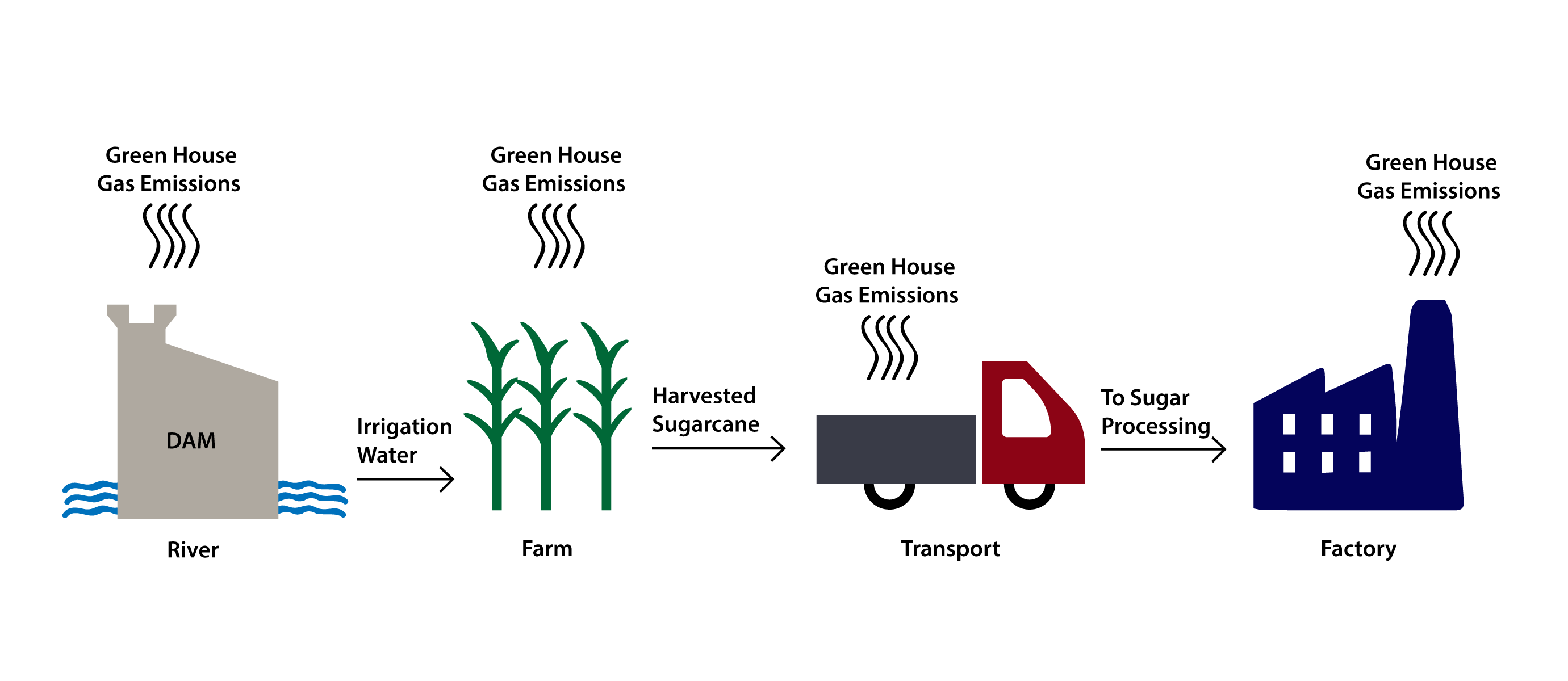
2.4. System Boundaries

This study system boundary includes four stages:
The reservoir phase which contains emissions fueled by pollution from decayed plants and saturated soils when the reservoir is first filled. The carbon in the plankton and plants that sprout and eventually decompose in the lake, the detritus eroded from the wetlands above, and the seasonal flooding of plants along the borders of the dam ensures that the reservoir’s pollution continues throughout its existence [16]. The emission levels vary widely depending on the area and condition of flooded vegetation, the size and shape of the lake, the local climate, and how the dam is managed [13].
The agricultural stage includes the following emission sources: fuel used for machinery, fertilizer, and pesticide production; nitrous oxide (N2O) emissions from the volatilization of nitrogen fertilizer (calculated as 1% of the N applied; [55]); energy utilization for irrigation; and equipment for harvesting and pre-harvest burning. Transportation stage emissions are consistent with the use of trucks to transport sugar cane to the factory (Figure 2). In The industrial stage (sugar milling and sugar conversion), the figure also shows emissions from electricity generation and fuel use.
Biomass combustion emissions are regarded as neutral because photosynthesis needs atmospheric carbon fixation throughout plant growth [56]. Only CH4 and N2O emissions were considered for the burning of biomass. In all cases, the agricultural fields had been cleared for subsistence farming prior to the establishment of the sugar district in 1982. As such, pre-impoundment land-use change emissions were only attributed to reservoir impoundment in the analysis, while pre-land use activities before the commencement of sugarcane cultivation were not considered.

2.5. Reservoir GHG Footprint Allocation

2.5.1. Allocation Method by Prairie YT, et al.

For a reservoir, the net annual GHG footprint is distributed amongst its various services.
Reservoirs provide some cultural, social, and environmental services:
  • Primary services: electricity, irrigation, water supply, flood control, fisheries, and environmental services.
  • Secondary services: growth-enabling food and water security, transport, recreation, climate mitigation, and more investment opportunities.
Emissions of GHGs must be assigned to each service, with allocation following a simple collection of provisions according to Prairie YT, et al. [13]:
  • The overall GHG emissions are allocated as follows: 80% for primary, 15% for secondary, and 5% for tertiary. If one allocation stage includes more than one function, the allocation for that stage is divided evenly between them.
  • Every allocation stage has a maximum of three services. This means a function of a lower allocation stage would never have a greater distribution than the service of a higher stage.
  • When no tertiary services are available, the allocation (5%) is divided between the secondary functions. The allocation (20%) is divided between the primary services if there is no secondary service.

2.5.2. Allocation Method by Scherer L, & Pfister S

Because reservoirs also serve many functions, irrigation alone should not be responsible for the environmental effects. Instead, the burden for the purposes of the reservoir should be shared. Allocation factors (fA) were, thus, introduced. These variables are founded on the rating of all the n functions that the reservoir sustains.
f A = n + 1 r a n k i n g i = 1 n i
where fA = allocation factor, n = number of reservoir purpose, and i = 1 n i = sum of rankings.

2.6. Life-Cycle Inventory

Data Collection

This study primarily encompasses agricultural irrigation practices, which include water withdrawal from a dammed river to sugarcane plantations, as well as the prevailing industrial operations in the sugar mill. The reservoir catchment data, including reservoir characteristics, catchment data, and pre-impoundment land cover in the area, were obtained from the Upper Benue River Basin Development Authority (UBRBDA) Yola, the literature, and the G-res tool. The sugarcane cultivation and sugar production data (2007–2017) were obtained from SSCL, the literature, and sugar company experts. Emissions from various process inputs, cane burning, and electricity from the power grid were also derived from literature and the BioGrace model. In 2011, BioGrace developed a list of additional standard values for a variety of inputs, process-related emissions, and modes of transport not specified in the BioGrace list of standard values or including more complex values. The BioGrace GHG framework consists of the BioGrace list of standard values, and it is so far the most up-to-date harmonized data background for Europe and the rest of the world [43,53]. The list provides a broader and more relevant background data for other parts of the world. It includes data on the selection of mineral fertilizer types and other agro-inputs, conversion inputs (process chemicals), national electricity grids, solid and gaseous biomass sources for energy, and transport [53]. See Table 1 and Table 2 for details, Table 3 for emission factors, and Table 4 for yearly sugarcane and sugar production statistics.

2.7. Study Limitations

This study scope focuses on incorporating the life-cycle GHG emissions of the reservoir into the carbon footprint of sugarcane irrigation/cultivation to sugar production. The manufacturing, transport and development of reservoir stages would contribute to emissions of GHGs. These emissions are a one-off source of GHG that can be traced to the reservoir services provided. Notice that temporary accommodation and worker movements are not specifically included, but in the “complete emissions” evaluation option they can be added by the user. As such, the net GHG footprint of the reservoir thus reflects a rational estimate of the actual emissions which are solely attributable to the impoundment of the reservoir. Although the G-res tool provides a detailed analysis of a reservoir’s lifetime emissions as an empirical tool, its implementation also has some drawbacks that may lead to the following uncertainty in results. Firstly, a custom factor was determined when an accurate emission factor was not available from a referenced source to match the material type used in the dam project. Secondly, only two out of possible four allocation approaches were considered in this study, due to data unavailability. Third, our model currently assesses only carbonic GHG emissions and does not take N2O emissions into account. In this sense, G-res can mainly be used as a warning mechanism to be used to determine whether the reservoir’s capacity for pollution is likely to be important or not. In the event of high expected emissions, more fieldwork and evaluation is often recommended. Lastly, the carbon footprint estimates from this study did not consider the factory wastewater treatment due to the lack of pollution leasing data. Only land-use change to reservoir creation was considered, since sugarcane land areas had been cleared for subsistent farming by the locals, prior to the establishment of the sugar district over 40 years ago [66].

2.8. Life-Cycle Impact Assessment

This is crucial to any LCA phase. A life-cycle impact assessment (LCIA) allows us to interpret data on emissions and resource utilization correlated with the life cycle of a product in aspects of environmental, public health, and resource constraints [67]. The greenhouse gases equivalencies model developed by EPA [52] was adopted for evaluating emissions from the agriculture, transport and industrial phases, while the G-res tool developed by the International Hydropower Association IHA in collaboration with UNESCO Chair of Global Environmental Change [13] was deployed. Based on the earlier defined functional unit, only the three significant greenhouse gases CO2, CH4 and N2O were considered for this study. Emission factors were taken from the BioGrace model since it is the most relevant and current standardized data background for Europe and the rest of the world [43,53].

2.8.1. Life-Cycle Reservoir GHG Emissions (G-Res Tool)

Contrary to direct measurements, empirical GHG footprint estimates of reservoirs are usually determined by applying averages of small flux measurements in adjacent lakes or streams that are assumed to be comparable [13]. Such approaches have the following limitations: It makes the assumption that observed systems are also representative of the entire “comparable” distribution of reservoirs; it does not take account of the particular environmental conditions of the specific reservoirs; the method suggests that GHG emissions are stable in time, although there is clear evidence that they decline dramatically in the early years after impoundment [68]; and it neglects the landscape’s GHG balance before flooding [13]. The need to quantify GHG emissions over 100 years or more, makes it essential to develop tools for predicting GHG emissions for long term reservoir projects, especially long-term climate change impacts [69]. This will differentiate between natural and reservoir-induced fluxes and thus lay the foundation for reporting for the anthropogenic GHG footprint of reservoirs, including those needed by foreign regulators [70]. The G-res tool uses a distinctive approach in its effort to reflect only the GHG emissions due to the expansion of the reservoir in a catchment. It is currently the most reliable method for assessing reservoir emissions based on LCA, due to its advantage of overcoming the above-highlighted limitations [13,71,72]. It was developed by the International Hydropower Association in partnership with UNESCO Chair for Global Environmental Change IHA [73], based on the recommendation from the Intergovernmental Panel on Climate Change [74]. The G-res tool uses readily available input data to estimate emission changes culminating from an existing reservoir or river intended for impoundment. The online tool takes human activity and construction emissions into account and allocates them to specific dam purposes [73]. The G-res tool is available online https://56.datatrium.com/fmi/webd#G-Res%20Tool and can be used free of charge. The web page includes technical documentation on the scientific basis for the tool and a guide for its step-by-step use.
The estimation of net carbon footprint in the G-res tool method includes emissions from four stages of the reservoir’s lifetime, using the following equation:
Net carbon footprint = Post-impoundment carbon balance of the reservoir] [Pre-impoundment carbon balance of the reservoir area before reservoir introduction] [Emissions from the reservoir due to unrelated anthropogenic sources (UAS)] + [GHG due to construction]
In the above mentioned equation, note the following:
  • Post-impoundment describes the emission of GHGs, including CO2 and CH4 diffusive, bubbling, and degassing for CH4, into the atmosphere over the reservoir basin after flooding, derived from a semi-empirical formula based on flow measurements from about 223 reservoirs globally [13].
  • Pre-impoundment takes into account the emissions within the area that the reservoir would fill.
  • Unrelated anthropogenic sources (UAS) suggest that the carbon emissions from human-induced activities in the reservoir region will be eliminated due to sewage. The reference here is the catchment area, the land area where rainfall gathers and flows off into a rising channel. This portion of emissions is estimated by using as a reference a portion of the phosphorus load that exceeds the normal background load [13].
  • Construction applies to emissions from the manufacture of materials, transport, and plant stages for dam construction and other related structures, determined from the use of materials and fuel, and also the associated emission factors [13].
It is important to note that the G-res tool was not designed as a validation tool for field measurements but to provide a comprehensive overview of the emissions over the lifetime of a reservoir [13]. The G-res tool requires the following inputs: upstream catchment data, area to be inundated by reservoir, and reservoir data. Details of the parameters are presented in Table 1.

2.8.2. Life-Cycle GHG Emissions of the Agriculture, Transport, and Industry Stages

At this stage, the EPA proposed a GWP system outlined in the latest scientific evaluation by IPCC that has been adopted for GHG estimation. The GWPs listed above are from the Fifth Assessment Report of the IPCC, which was published in 2014 [1], and they are based on the carbon footprint assessment framework [52].
  • Cane trash burning emission
C T B e m i s s i o n = H A × E F C T × Y S C Y S G
CTBemission = cane trash burning emission (kg CO2-eq/kg), HA = harvested area to burnt trash (ha), EFCT = emission factor for cane trash (kg CO2-eq/kg dry matter), YSC = total sugarcane yield (tons/ha), and YSG = total sugar yield (tons).
  • Diesel emissions (field)
D F e m i s s i o n = E F d i e s e l × R d i e s e l × L H V d i e s e l × A Y S G
DFemission = field diesel emission (kg CO2-eq/kg), EFdiesel = diesel emission factor (kg CO2-eq/MJ), Rdiesel = rate of diesel consumption (L/ha), LHVdiesel = lower heating value (MJ/L), A = total land area harvested (ha), and YSG = total sugar yield (tons).
  • Chemical application emissions
According to the field manual for cane cultivation from the agricultural department of SSCL, chemical fertilizer is typically applied 2 or 3 times for the entire cropping period. The recommended fertilizer rate for this study plant cane is 150–60–60 kg/ha, applied as follows: NPK, 15–15–15 eight bags/ha in the furrow and covered during planting; and UREA 46% four bags/ha in the furrow during hill-up (10–12 WAP), and additional (18–20 WAP) as per agronomy suggested. Alternatively, Di-Ammonium-Phosphate (DAP) 18–46–0 three bags/ha in the furrow and protected during planting. N fertilizer application can result in direct and indirect emissions of N2O from soil [51].
C A e m i s s i o n s = R C A × E F C H × A Y S G
CAemissions = chemical application emissions (kg CO2e/kg), RCA = chemical application rate (%), EFCH = chemical emission factor (g CO2-eq/kg), A = total land area harvested (ha), and YSG = total sugar yield (tons).
  • Diesel emission (transportation)
D T e m i s s i o n s = R d i e s e l × E F d i e s e l × L H V d i e s e l × T S C Y S G
DTemissions = transportation diesel emissions (kg CO2-eq/kg), Rdiesel = rate of diesel consumption (L/ton), EFdiesel = diesel emission factor (kg CO2-eq/MJ), LHVdiesel = lower heating value (MJ/L), TSC = tons of sugarcane transported (tons), and YSG = total sugar yield (tons).
  • Bagasse emissions
B G e m i s s i o n s = T B G × E F B G Y S G
BGemissions = bagasse emissions (kg CO2-eq/kg), TBG = tons of bagasse combusted (tons), EFBG = emission factor of bagasse (kg CO2-eq/kg), and YSG = total sugar yield (tons).
  • Lubricants emissions
L B e m i s s i o n s = R L B × E F L B × A Y S G
LBemissions = lubricant emissions (kg CO2-eq/kg), RLB = rate of lubricants consumption (kg/ha), EFLB = lubricants emission factor (kg CO2-eq/kg), A = total land area harvested (ha), and YSG = total sugar yield (tons).
  • Fuel oil emissions
F O e m i s s i o n s = R F O × E F F O × L H V F O × T S C Y G
FOemissions = fuel oil emissions (kg CO2-eq/kg), RFO = rate of fuel oil consumption (L/ton), EFFO = fuel oil emission factor (kg CO2-eq/MJ), LHVFO = lower heating value (MJ/L), TSC = tons of sugarcane Produced (tons), and YSG = total sugar yield (tons).
  • Electricity grid emissions
E G e m i s s i o n s = E I × E F E Y S G
EGemissions = emissions from electricity grid (kg CO2-eq/kg), EI = electricity imported (KWh), EFE = electricity emission factor (kg CO2-eq/KWh), and YSG = total sugar yield (tons).

2.8.3. Total Lifetime GHG Emission

The total lifetime GHG emission from the defined system boundary can thus be simply estimated for the 100-year lifetime as follows:
G H G t o t a l = G H G r e s e r v o i r + G H G a g r i c u l t u r e + G H G t r a n s p o r t + G H G f a c t o r y

2.9. Statistical Analysis

A simplified linear regression analysis was performed to correlate both models for allocation of open reservoir GHG emissions. It is given by (Ec,u = μu × Em,u), where Ec,u is the allocated reservoir GHG emission by Prairie et al., 2017 u (t CO2e·month−1), Em,u is the allocated reservoir GHG emission by Scherer and Pfister, 2016 u (t CO2e·month−1) and μu is the regression coefficient for the reservoir emission u. In order to determine the output of both allocation methods, the root mean square error (RSMEu) was also determined and the determination coefficient of this regression.
R S M E u = 1 m v = 1 12 ( E m , u , v E c , u , v ) 2
where Em,u and Ec,u are already defined, subscript v indicates different monthly values, and 12 is the total number of months from January to December.

2.10. Sensitivity Analysis

Several sources of uncertainty will affect the results of a life-cycle assessment (LCA) analysis, largely related to the analytical choices, early assumptions, i.e., allocation rules, system boundaries and techniques of impact assessment, and the consistency of existing data [75]. Sensitivity analysis (SA) is a valuable method in the life-cycle assessment (LCA) to test the robustness of outcomes and their responsiveness to uncertainty factors. It emphasizes the very critical set of model variables to decide whether data accuracy ought to be enhanced and to improve results understanding [76]. LCAs demand several input data, and most of these variables are uncertain, so a sensitivity analysis is a key component of final interpretation. In this study, sensitivity analysis for the reservoir emissions is evaluated by using the G-res tool based on the influence rate of post impoundment decomposition of biomass on carbon emission intensities over reservoir lifetime. Secondly, it considers the impact of seasonal weather fluctuations with combined irrigation and potential 20 MW hydroelectric power operation on the existing reservoir [50]. Furthermore, a potential development in the sugar district that will improve the sugar milling capacity by about 260,000 tons of sugar per year, from sugar cane grown on around 25,000 hectares of agricultural land [77] is assessed for the other phases.

3. Results

3.1. Allocation of Reservoir GHG Footprint

Simple regression analysis (Figure 3) shows a good performance of the two GHG allocation models proposed by Prairie YT, et al.; Scherer L, & Pfister S. [13,15]. For both allocation methods, root mean square errors (RSME) values were less than 534.35 t CO2e/month, while the relative errors of the calculated monthly open water reservoir GHG emission were all below 8% and mean value of ~1%. Both allocation models had an average RMSE of 510.50 and 511.65 t CO2e/month, respectively, which is an indication that both models had strong correlation, hence the model by Prairie et al., 2017, was utilized in estimating and reporting reservoir GHG emission.

3.2. GHG Emissions from the Reservoir

3.2.1. Pre-Impoundment GHG Balance of the Reservoir Area

The ecosystem flooded after impoundment by a reservoir is a mixture of different ecological sub-components: forests, wetlands, agricultural areas, cities, lakes, streams, and, most definitely, the main river. Pertinent to the intensity of land use and GHG balances, each of these sub-components may exhibit certain comportment. While a section of forest absorbs typically CO2 from the atmosphere by photosynthesis, for instance, wetlands in addition to depositing carbon as peat also commonly emit CH4 like rivers, lakes, and natural streams. Estimates from this study have shown that significant Greenhouse gases, primarily methane (CH4) ~2538 t CO2-eq/yr and carbon dioxide (CO2) ~14,044 t CO2-eq/yr, are emitted annually from the reservoir as a result of impoundment in 1978. Results further indicate that prior to the creation of the reservoir, approximately 16,582 t CO2-eq/yr GHG was emitted annually from the water body.

3.2.2. Post-Impoundment GHG Balance of the Reservoir

Due to the decomposition of organic material in the flooded area, greenhouse gases can indeed be emitted over time when a reservoir is formed [73]. In these processes, the carbon stored interacts with the environment primarily through three processes. First of all, the major source of emission is diffusive flux occurring on the water surface. CH4 diffusive flux is largely dependent on the reservoir temperature and spatial variables from the empirical model in the G-res tool, while CO2 diffusive flux is also influenced by the carbon content of the soil surface. Furthermore, bubbling with CH4 is dependent on the reservoir’s horizontal surface radiance and other geographical parameters. Lastly, the release of water from the deeper upstream to the downstream through the water intake channel for purposes such as hydroelectricity generation and environmental flow could result in degassing (release of GHG). The gross CH4 emissions after impoundment are obtained as the sum of the three different forms of CH4 emissions: CH4 diffusive emissions after impoundment, CH4 bubbling emissions, and CH4 degassing emissions. The reservoir’s area rate of emission after impoundment is 604 g CO2/m2/yr for CO2, and 1517 g CO2/m2/yr for CH4, while uncertainty pertinent to carbon footprints for total lifespan at 95% confidence intervals is 45% for diffusive flux, 35% for degassing and 20% for bubbling respectively. Post-impoundment life-cycle emissions sum up to 265,419 t CO2-eq/yr. In terms of reservoir services, the explicit prioritization method of allocating importance to the services [13] has shown that irrigation, which is the primary service purpose of the reservoir accounts for an annual GHG footprint of 51,298 t CO2-eq/yr, environmental flow, which is the secondary purpose, emits 9618 t CO2-eq/yr of GHG and lastly fishing and recreation which are both tertiary purposes, each account for 1603 t CO2-eq/yr Table 5.

3.2.3. Emissions from the Reservoir Due to UAS

Unrelated anthropogenic sources (UAS) account for 185,046 t CO2-eq/yr because the population density of the catchment is less than 100 persons/km2, with only no more than 1% of the settlement area and croplands mainly rainfed in all catchments. The managed rates of all land type inputs for the G-res tool are set at low, resulting in a net GHG footprint of 64,122 t CO2-eq/yr. Table 6 represents the CH4 release rate due to UAS, whereby the water residence time corresponds to the mean period that a water molecule spends in the reservoir.

3.2.4. GHG Emissions Due to Construction

The construction of the dam, which includes infrastructures and equipment comprising of different materials, such as steel, stainless steel, iron, and copper, will need tremendous quantities of energy at this level to carry and install, leading to emissions that constitute a one-off GHG source. The contribution of the construction stage of the reservoir/dam to the total lifetime emission is equal to 33,060 t CO2-eq.

3.2.5. Net GHG Footprint

The net GHG footprint is the sum of the four sections described above, as per Equation (1). Total lifetime emission of the reservoir amounts to 6,412,182 t CO2-eq, of which 16,582 t CO2-eq/yr is allocated to pre-impoundment, 265,419 t CO2-eq/yr to post-impoundment, 64,122 t CO2-eq/yr to UAS and 33,060 t CO2-eq to construction. This results in a reservoir carbon footprint of 5.04 kg CO2-eq/kg for sugar, representing 80% of total lifetime GHG emissions in this study case Table 7.

3.3. GHG Emissions from the Agricultural Stage (Cultivation)

3.3.1. GHG from Energy Use in Farming Operation

In this study, GHGs emissions from the utilization of fossil fuel energy for sugarcane cultivation has been estimated. Tillage, which is the major energy consumer at this stage, is carried out mechanically with the use of tractors. The total annual diesel consumption for this study case is 127 L/ha/y, of which 99 L/ha/y is allocated to tillage practices, 14 L/ha/y to insecticide application, 10.2 L/ha/y to irrigation and 3.8 L/ha/y to herbicide application respectively. GHG emissions were estimated for the utilization of fossil fuel for these phases, and results reveal that emissions from diesel use are as follows: 0.117 kg CO2-eq/kg for tillage, 0.017 kg CO2-eq/kg for insecticide, 0.012 kg CO2-eq/kg for irrigation, and 0.0045 kg CO2-eq/kg for herbicide application, respectively. Thus, the overall GHG emission for the sugarcane cultivation stage is 0.150 kg CO2-eq/kg, which accounts for 2.2% of total lifetime GHG emission in this stage.

3.3.2. GHG Emissions from Fertilizer Application

Direct emissions were estimated from N application through synthetic fertilizer and organic fertilizer. Additionally, direct CO2 emissions from the application of urea were estimated. On the basis of 1% of N to N2O [55], N emission from direct emissions was calculated as 0.106 kg CO2-eq/kg from NPK, 0.2843 kg CO2-eq/kg from DAP, and 0.163 kg CO2-eq/kg from UREA respectively, yielding a total N2O direct emission of 0.00284 kg CO2-eq/kg, P2O5 emission of 0.145 kg CO2-eq/kg and K2O emission of 0.106 kg CO2-eq/kg. GHG emission from fertilizer application amounts to 0.254 kg CO2-eq/kg, which equals to 3.7% of total lifetime GHG emissions at this stage.

3.4. GHG Emissions from Transportation of Sugarcane to the Sugar Factory

Harvested sugarcanes are transported to the sugar factory by the use of trucks that utilize diesel fuel. The GHG emissions from the use of such fuel were estimated the same way as was done during the cultivation stage. The rate of fuel consumption from the farms to the sugar factory is 1.26 L/ton of cane conveyed. The GHG emission at this stage resulted in 0.065 kg CO2-eq/kg, which accounts for approximately 1.5% of total lifetime emissions.

3.5. GHG Emissions from Biomass Burning

Usually, two kinds of burning, pre-harvest and post-harvest burnings, occur in some sugarcanes producing regions around the world. Pre-Harvest burning is highly discouraged because it reduces sugar quality in addition to its air pollution potentials. The fraction of farm areas burned annually equals 96% of the total land area harvested, which is equivalent to 163,469 tons of cane. Greenhouse gases emissions from biomass burning include CH4 and N2O, which, if converted to CO2, results in an emission factor of 1.085 kg CO2-eq/kg dry matter [65]. The total GHG emission from biomass burning activities obtained is 0.016 kg CO2-eq/kg, which is 0.23% of overall lifetime emissions.

3.6. GHG Emissions from the Sugar Factory

Background information obtained for this study indicates that the sugar factory highly relies on bagasse to generate electricity to supplement incessant electricity supply shortages attributed to the region. Reports reveal that over 50% of the total electricity consumption of the factory comes from bagasse. The amount of bagasse in cane burned annual is approximately 42%, which is equivalent to 69,513 tons of cane per year, thus, resulting in a carbon footprint of 0.171 kg CO2-eq/kg. Electricity imported from the grid is equal to 0.17 kWh/ton cane, yielding a GHG emission of 0.0005 kg CO2-eq/kg, which, compared to that of bagasse, signifies the heavy dependence on bagasse for energy generation. The use of fuel oil to supplement energies from bagasse and the grid is 0.75 L/ton cane, which results in a carbon footprint of 0.04 kg CO2-eq/kg.
In contrast, the use of lubricants and lime in production processes results in GHG emissions of 0.000166 kg CO2-eq/kg and 0.0153 kg CO2-eq/kg, respectively. Bagasse burning is the major contributor to overall GHG emission at this stage, accounting for 75% of total emissions. In terms of overall lifetime emissions, the factory accounts for 3.5% of total GHG emissions.

3.7. Overall Lifetime GHG Emissions from All Stages

Total lifetime GHG emission from the system boundary, summing up emission from the reservoir, sugarcane cultivation, transportation, and sugar factory, amounts to 5.76 kg CO2-eq/kg cane, of which the reservoir accounts for the largest share of emissions 5.04 kg CO2-eq/kg cane (87%), followed by the agriculture stage 0.430 kg CO2-eq/kg (7.5%), and then sugar production 0.227 kg CO2-eq/kg (3.5%) and lastly the transportation stage 0.065 kg CO2-eq/kg (1.5%). Fossil fuels account for approximately 35% of overall life-cycle emissions, while non-fossil fuels 26% and chemical application 39% (Figure 4).

3.8. Sensitivity Analysis Outcomes

The findings of the scenario study indicate that there are significant variations in GHG emissions, taking into consideration post-impoundment, UAS, as well as the overall construction activities. Comparing total reservoir construction emissions, it is noted that emissions associated with dam construction remain constant, while the other parameters’ annual balance is relatively small, though accumulated over time [71]. Therefore, the GHG intensity (GHG emissions per unit of sugar produced/electricity generated) is based on the multipurpose dam’s total lifetime. GHG intensity is determined based on the planned annual productivity Table 1 when the lifespan ranges from 10 to 100 years in Figure 5a. It falls rapidly when lifespan increases by 10 to 50 years in both scenarios, and then slightly decreases, with lifespan increasing. GHG intensity reaches 0.73 kg CO2-eq/kg for sugar, and 1.01 t CO2-eq/MWh for hydroelectricity as the lifespan attains 100 years. This implies that reservoirs would have relatively higher GHG intensities if they run for less than 40 years and are more efficient and cleaner if they stay in good health for much over 50 years.
On the basis of concurrent use of the reservoir for irrigation and hydropower generation, operations will last more than 70% of the year at or about maximum output. At this time, the output will be restricted only by a drawdown at a normal operating level due to the tailwater during the increased flow months or by flows retained to the full storage level of the Kiri dam reservoir [66]. For 25% of the year, when the reservoir runs at less output, drawdown (170.5 m–96 m) leads to increasing carbon intensities 0.058 to 0.102 t CO2-eq/month during the driest 15% of the year. However, during the driest 35% (about four months) of the year, carbon intensity would average about 0.580 t CO2-eq/month, as can be seen in Figure 5b. During the driest 10% of the year, when combined irrigation and energy demand would be much higher, reservoir drawdown (96 m–60 m) leads to increased carbon intensity from 0.573 t CO2-eq/month to about 0.680 t CO2-eq/month, Figure 5b. Although reservoir drawdown areas that are regularly dry and then flooded may abnormally facilitate reservoir-wide GHG emissions due to fluctuating redox reactions [78,79], drawdown can also be a critical hotspot period for reservoir-wide CH4 release as hydrostatic pressure decreases may cause ebullition events as observed in this sensitivity analysis and earlier reported by Maeck A, et al. [80].
Finally, there is a clear indication that sugarcane productivity per hectare of cultivated land in the district is below average, based on current operating conditions. Substantial differences compared to future scenario also indicates that less sugarcane is produced on vast hectares of land on the basis of sugar recovery rate. As for the reservoir GHG emissions, the potential incorporation of hydropower to the existing dam significantly reduced emission to irrigation from 5.04 kg CO2-eq/kg to 0.196 kg CO2-eq/kg as elucidated above. Therefore, incorporating more functions to a reservoir will influence the GHG emission of its various services substantially Table 8. In all scenarios compared, CF of sugar production is largely influenced by parameters of the reservoir phase (lifespan emissions).

4. Discussion

The average GHG emission rate for this study reservoir of surface area 25,000 km2 is 0.0658 Tg CO2-eq/year of CO2 and 0.172 Tg CO2-eq/year of CH4 regardless of the priority of purpose assigned to the reservoir. Compared to global estimates, GHG emission from reservoirs could range from 45 to 1000 Tg CO2-eq/year of CO2 and 135 to 2380 Tg CO2-eq/year of CH4, with reservoir area ranging from 350,000 to 1,500,000 km2 [6,70]. This corroborates the evidence that areal fluxes and reservoir surface area are a critical determining factor to the emission rate of GHGs from reservoir surfaces, regardless of the geographical location [16]. Though the GWPs for CO2-equivalent estimations were mostly reported over 100 years, the choice of periods is somewhat ambiguous in the sense that CH4 is comparatively temporary in atmosphere comparative to CO2 and thus has a higher GWP over the shorter 20-year timescale [81]. Our estimates further show that potential GHG emissions to hydropower generation are approximately 6144 kg CO2-eq/MWh, which compared to estimates by Räsänen TA, et al. [27] for the Mekong river basin is about four-fold 22,000 kg CO2-eq/MWh for hydropower reservoirs which supported irrigation. However, emissions range from 0.2–1994 kg CO2-eq/MWh for reservoirs solely generating hydroelectric power, while emission fluxes range from 26–1,813,000 t CO2-eq/yr over a 100-year lifetime [27]. In major tropical reservoirs around the world, CO2 diffusive fluxes range from −38.9 to 70 mg/m2/d in Laos, 1684 mg/m2/d this study, −440 to 16,280 mg/m2/d in French Guiana. While for Brazil, which is the water resource richest country in the tropics and world, CO2 diffusive fluxes range from 171 mg/m2/d in Itaipu to as high as 13,845 mg/m2/d in Balbina [29]. While diffusion is predominant means for the emission of CO2 from reservoirs, bubbling fluxes of CO2 in the tropics range from 0 mg/m2/d in Balbina, 0.44 mg/m2/d this study, to as high as 3.76 in Três Marias [29]. This clearly shows that ebullition has significantly little contribution to the emission of CO2 from reservoir surfaces, due to its large solubility of CO2 [22].
In temperate regions of the world, however, CO2 continues to be the dominant diffusive flux in reservoirs with a peak flux of 7150 mg/m2/d for CO2 and CH4 flux of 3850 mg/m2/d both in southeast Poland [29]. Ebullition, however, continues to be less significant, like in the tropics. Comparing our estimates to recent studies in China which employed the G-res tool indicate that average CF for large hydropower plants is 7.25 t CO2-eq/GWh for 100 years [71,72], compared to 6773 t CO2-eq/GWh a smaller hydropower plant in this study. This suggests that larger hydropower plants do not necessarily correspond to any significant increase in carbon emission intensity. While hydroelectric dams continue to dominate GHG emission from reservoirs globally, constituting 30–62% of global impoundments [9,82]. The GHG report by Deemer BR, et al. [16] suggests that 82% of studied reservoirs have the potential for hydroelectricity generation. As such, no significant differences were observed between GHG emissions of hydropower versus non-powered dams/reservoirs. While regional disparities continue to attribute to variations in CF of reservoirs, CO2 emissions from reservoirs will always be influenced by the flooded organic matter, water temperature, geographic location of reservoirs, reservoir age, pH value, vegetation, and wind speed. Hence, the application of varying approaches will inevitably be limited by uncertainties, depending on the reservoir’s lifespan.
Comparison of the three other stages, agriculture, transportation, and sugar production to other studies, have shown that CF values of this study are relatively high in regards to sugar recovery rate. A case study in brazil reported CF values of between 0.23 and 0.24 kg CO2-eq/kg sugar [64,83], in Mauritius, CF of sugar reached 0.255 kg CO2-eq/kg sugar [84], while in Thailand, Yuttitham M, et al. [45] reported 0.55 kg CO2-eq/kg sugar and most recently Mexico 0.45–0.63 kg CO2-eq/kg sugar.
In all the aforementioned studies, the highest GHG emissions occur in the agricultural stage and are dominated by nitrogenous fertilizer use and cane burning during harvest. Differences in the fertilizer use rate for cultivation is probably responsible for the disparity in carbon footprint at this stage. Fertilizer use rates could be as high as 199 ± 203 kg N/ha for eastern Thailand, 75 kg N/ha for brazil, and ~60 kg N/ha for this study. Another reason for the relatively high carbon footprint at the agricultural stage in this study is the low productivity of sugarcane. The average cane yield in this study is 45 tons/ha and GHG emission of 0.43 kg CO2-eq/kg sugar, while in Mexico, average cane yield is 90 ton/ha and GHG emission of 0.33 kg CO2-eq/kg sugar [43]. This indicates the need to increase sugarcane yield per unit area of land to curb greenhouse gas emissions per unit of sugar produced, as also reflected in the sensitivity analysis. GHG emissions from cane trash burning are 0.016 kg CO2-eq/kg sugar, accounting for 0.0023% of total lifetime GHG emissions, which seem relatively insignificant compared to other stages. However, the future scenario shows that the carbon footprint of cane burn can reduce significantly to 0.0045 kg CO2-eq/kg sugar, while cane productivity can be maximized. Compared to other studies, emissions from cane burning in brazil is 0.048 kg CO2-eq/kg sugar, accounting for 65% of total harvested area, 0.10 kg CO2-eq/kg sugar in Mexico, accounting for 89–95% of harvested area, 0.05 kg CO2-eq/kg sugar and 51% of the harvested area and this study 96% of harvested area. Differences in emissions are attributable to the fact that burning is assigned not only to sugar production but ethanol production as well in places such as Brazil. Adopting green harvest methods as an alternative to cane burning [85], utilization of sugarcane trash for livestock feeding [86], can significantly reduce greenhouse gas emissions at this stage.
The transportation stage seems much less significant compared to other stages. It accounts for just 1% of overall emissions, while it could up 6.3% in the future. While it ranges between 10 and 13% of the total GHG emissions in Mexico [43]. The industrial stage accounts for a mere 3.3% of total lifetime emissions for the base case scenario, which could reach 6.3% in future expansion. GHG emissions for this study are 0.23 kg CO2-eq/kg sugar base case scenario, which compared to other studies is relatively high but could decrease with better practices in the future. It ranged from 0.07 to 0.20 kg CO2-eq/kg sugar [43], while in Thailand, it was relatively lower [45]. Significantly higher values of GHG emissions in the study and some parts of Mexico could be attributed to the fact that the sugar factories are reliant on fossil fuel use to supplement erratic power supply from the grid, especially in this study case. Overall, disparities in results of carbon footprints of sugar from relevant studies, depending on the material and energy inputs, and also the type of data available for selection to perform these estimates.
By combining the G-res tool modelling approach with the EPA approach by IPCC for scientific evaluation for GHG estimation, this study presents a more comprehensive framework for evaluation of GHG emissions from a reservoir and a more precise quantification of the carbon footprint of an irrigated food product. In its attempt to reflect only the GHG emissions due to the deployment of the reservoir in a catchment, the G-res tool uses a unique method. Thus, we applied simple conceptual equations within these concepts to describe the net GHG footprint as seen in the Equation (11). Our approach provides a basis for incorporating reservoir GHG emissions into the carbon footprint of an end product dependent on a reservoir function, growing awareness as to how a region utilizing its water resources is contributing to global GHG emissions and climate change. This methodology could also be useful for planning of other projects requiring reservoir storage, and can be applied to multipurpose reservoirs to understand the carbon footprint of its various consumptive uses. The framework described in this study can be used by policymakers concerned with the effects of water resources and climate change to make an effective cost-benefit analysis of potential water storage and use projects by integrating environmental and socioeconomic benefits. This will be exceptionally critical as the effect of climate change, population and economic growth on the water-energy-food nexus increases the reliance on water storage reservoirs in most regions of the world.

5. Conclusions

In this study, we have underlined the need to incorporate reservoir GHG emissions into CF of sugar production, adopting the LCA method. This is because large amounts of GHG emissions are associated with reservoirs impounded for irrigation agriculture and other purposes. While results have revealed that significantly large number of GHG emissions are associated with reservoir impoundment which could allocate up to 80% of total GHG emissions to the primary purpose of the reservoir, sensitivity analysis reveals that GHG intensity is mostly dependent on lifespan of the reservoir, especially in the early decades of impoundment driven by biomass decomposition rate and seasonal climatic variations. To limit uncertainties, the novelty of this approach integrates not only the gross GHG fluxes but also takes into cognizance the condition of the river and natural environment prior to impoundment. Furthermore, it considers the integrated impact of reservoir aging, considers GHG emissions to the construction phase, and eliminates emissions due to unrelated anthropogenic sources UAS in gross measurements. This approach can be applied to other regions of the world, to comprehend how multipurpose reservoirs influences the CF of the end products of its respective purposes.
The following coping measures, however, would be crucial to curtailing GHG pollution in the sugar district:
(i)
Significantly large GHG emissions from the reservoir could be reduced in terms of service purposes when more services are allocated to the reservoir.
(ii)
Coupled with improving sugarcane productivity per hectarage of cultivated land, GHG emissions at the agricultural stage can be curbed by adopting green harvest rather than cane burning.
(iii)
The industrial stage could use more bagasse to generate energy rather than fossil fuels, to promote cleaner and efficient generation.
As the global need for sustainable food production is extensively dependent on irrigation for a booming population, the implementation of large-scale river development projects for food, energy, and other purposes will continue to increase. It is, hence, crucial to understand how water withdrawn from reservoirs for irrigation contribute not just to reservoir wide GHG pollution, but also how life-cycle GHG emissions from multipurpose reservoirs influence the total carbon footprints of the respective end products of its various functions. We further stress the need to incorporate socioeconomic aspects of LCA in future studies, to holistically inform stakeholders. Finally, it is imperative for policymakers to comprehend and make plans for the growing tradeoffs amongst key functions of irrigated sugarcane-sugar production and other irrigated food products. This will be particularly critical as the agro-hydrological consequences of climate change, demographic and economic growth, and related lifestyle changes boost the need for irrigated agriculture and food production in most regions of the world. Towards environmental sustainability and transition to a low carbon future, this study could be a reference to other regions where rivers have been impounded or intend to be impounded for food commercialization and other purposes.

Author Contributions

Conceptualization, T.K.Y. and Y.L.; methodology, T.K.Y.; software, T.K.Y.; validation, T.K.Y., Y.L. and B.S.L.; formal analysis, B.S.L., G.W.D.; investigation, G.W.D.; resources, G.W.D.; data curation, B.S.L.; writing—original draft preparation, T.K.Y.; writing—review and editing, T.K.Y.; visualization, T.K.Y. supervision, Y.L.; project administration, T.K.Y.; funding acquisition, Y.L. All authors have read and agreed to the published version of the manuscript.

Funding

This study was supported by the National Key R&D Program of China (No. 2019YFC0408301), the National Natural Science Foundation of China (No. 51779076); the Foundation for Innovative Research Groups of the National Natural Science Foundation of China (No. 51421006); the Six Talent Peaks Project in Jiangsu Province (2016-JNHB-007); and the 333 Talent Project Foundation of Jiangsu Province and the Priority Academic Program Development of Jiangsu Higher Education Institutions (PAPD).

Conflicts of Interest

The authors declare no conflict of interest.

References

  1. IPCC. Climate Change 2014: Impacts, Adaptation and Vulnerability; IPCC: Cambridge, UK, 2014. [Google Scholar] [CrossRef] [Green Version]
  2. Paul, G.; Harris, P.G. Climate change. Clim. Chang. 2011, 20, 107–118. Available online: https://atlascorps.org/climate-change/ (accessed on 20 June 2019).
  3. United Nations. Climate Change, The Human Fingerprint on Greenhouse Gases. 2013. Available online: https://www.un.org/en/sections/issues-depth/climate-change/ (accessed on 15 July 2019).
  4. Caro, D. Carbon Footprint. Encycl. Ecol. 2019, 201, 252–257. [Google Scholar] [CrossRef]
  5. Demarty, M.; Bastien, J. GHG emissions from hydroelectric reservoirs in tropical and equatorial regions: Review of 20 years of CH4 emission measurements. Energy Policy 2011, 39, 4197–4206. [Google Scholar] [CrossRef]
  6. St. Louis, V.L.; Kelly, C.A.; Duchemin, É.; Rudd, J.W.M.; Rosenberg, D.M. Reservoir Surfaces as Sources of Greenhouse Gases to the Atmosphere: A Global Estimate. Bioscience 2000, 50, 766. [Google Scholar] [CrossRef]
  7. Downing, J.A.; Prairie, Y.T.; Cole, J.J.; Duarte, C.M.; Tranvik, L.J.; Striegl, R.G.; McDowell, W.H.; Kortelainen, P.; Caraco, N.F.; Melack, J.M.; et al. The global abundance and size distribution of lakes, ponds, and impoundments. Limnol. Oceanogr. 2006, 51, 2388–2397. [Google Scholar] [CrossRef] [Green Version]
  8. Lima, I.B.T.; Ramos, F.M.; Bambace, L.A.W.; Rosa, R.R. Methane emissions from large dams as renewable energy resources: A developing nation perspective. Mitig. Adapt. Strat. Glob. Chang. 2007, 13, 193–206. [Google Scholar] [CrossRef]
  9. Lehner, B.; Liermann, C.R.; Revenga, C.; Vorosmarty, C.J.; Fekete, B.M.; Crouzet, P.; Döll, P.; Endejan, M.; Frenken, K.; Magome, J.; et al. High-resolution mapping of the world’s reservoirs and dams for sustainable river-flow management. Front. Ecol. Environ. 2011, 9, 494–502. [Google Scholar] [CrossRef] [Green Version]
  10. World Bank Group. Greenhouse Gases from Reservoirs Caused by Biogeochemical Processes; World Bank Group: Washington, DC, USA, 2017. [Google Scholar] [CrossRef]
  11. Barros, N.; Cole, J.J.; Tranvik, L.J.; Prairie, Y.T.; Bastviken, D.; Huszar, V.L.M.; Del Giorgio, P.; Roland, F. Carbon emission from hydroelectric reservoirs linked to reservoir age and latitude. Nat. Geosci. 2011, 4, 593–596. [Google Scholar] [CrossRef]
  12. Raymond, P.A.; Hartmann, J.; Lauerwald, R.; Sobek, S.; McDonald, C.; Hoover, M.; Butman, D.; Striegl, R.; Mayorga, E. Erratum: Global carbon dioxide emissions from inland waters. Nature 2014, 507, 387. [Google Scholar] [CrossRef] [Green Version]
  13. Prairie, Y.T.; Alm, J.; Harby, A.; Mercier-Blais, S.; Nahas, R. The GHG Reservoir Tool (G-res) Technical documentation, UNESCO/IHA research project on the GHG status of freshwater reservoirs. Version 1.12. Joint publication of the UNESCO Chair in Global Environmental Change and the International Hydropower Association. 2017. Available online: https://assets-global.website-files.com/5f749e4b9399c80b5e421384/5fa83c07d5f3c691742fd0d8_g-res_technical_document_v2.1.pdf (accessed on 23 November 2020).
  14. IHA. Hydropower Emissions. In Proceedings of the World Hydropower Congress, Addis Ababa, Ethiopia, 9–11 May 2017. [Google Scholar]
  15. Scherer, L.; Pfister, S. Hydropower’s biogenic carbon footprint. PLoS ONE 2016, 11, e0161947. [Google Scholar] [CrossRef] [PubMed] [Green Version]
  16. Deemer, B.R.; Harrison, J.A.; Li, S.; Beaulieu, J.J.; DelSontro, T.; Barros, N.; Bezerra-Neto, J.F.; Powers, S.M.; Dos Santos, M.A.; Vonk, J.A. Greenhouse gas emissions from reservoir water surfaces: A new global synthesis. Bioscience 2016, 66, 949–964. [Google Scholar] [CrossRef] [PubMed]
  17. Bastviken, D.; Tranvik, L.J.; Downing, J.A.; Crill, P.M.; Enrich-Prast, A. Freshwater methane emissions offset the continental carbon sink. Science 2011, 331, 50. [Google Scholar] [CrossRef] [PubMed] [Green Version]
  18. Hertwich, E.G. Addressing biogenic greenhouse gas emissions from hydropower in LCA. Environ. Sci. Technol. 2013, 47, 9604–9611. [Google Scholar] [CrossRef] [PubMed]
  19. Fearnside, P.; Rosa, L.P.; Saut, P.; Guiana, F.; Paris, T.; Nations, U. Methane Quashes Green Credentials of Hydropower Preprint Analysis Quantifies Scientific Plagiarism. Nature 2006, 444, 524–525. [Google Scholar]
  20. Fearnside, P.M.; Pueyo, S. Greenhouse-gas emissions from tropical dams. Nat. Clim. Chang. 2012, 2, 382–384. [Google Scholar] [CrossRef]
  21. Giles, J. Methane quashes green credentials of hydropower. Nat. Cell Biol. 2006, 444, 524. [Google Scholar] [CrossRef]
  22. Rosa, L.P.; Dos Santos, M.A.; Matvienko, B.; Sikar, E.; Dos Santos, E.O. Scientific errors in the fearnside comments on greenhouse gas emissions (GHG) from hydroelectric dams and response to his political claiming. Clim. Chang. 2006, 75, 91–102. [Google Scholar] [CrossRef]
  23. Fearnside, P.M. Greenhouse gas emissions from Brazil’s Amazonian hydroelectric dams. Environ. Res. Lett. 2016, 11, 011002. [Google Scholar] [CrossRef]
  24. Steinhurst, W.; Knight, P.; Schultz, M. Hydropower Greenhouse Gas Emissions: State of the Research; Synap Energy Econ Inc.: Cambridge, MA, USA, 2012; pp. 1–23. [Google Scholar]
  25. Zhao, Y.; Wu, B.F.; Zeng, Y. Climate of the Past Geoscientific Instrumentation Methods and Data Systems Spatial and temporal patterns of greenhouse gas emissions from Three Gorges Reservoir of China. Biogeosciences 2013, 10, 1219–1230. [Google Scholar] [CrossRef] [Green Version]
  26. Almeida, R.M.; Shi, Q.; Gomes-Selman, J.M.; Wu, X.; Xue, Y.; Angarita, H.; Barros, N.; Forsberg, B.R.; García-Villacorta, R.; Hamilton, S.K.; et al. Reducing greenhouse gas emissions of Amazon hydropower with strategic dam planning. Nat. Commun. 2019, 10, 4281. [Google Scholar] [CrossRef] [PubMed]
  27. Räsänen, T.A.; Varis, O.; Scherer, L.; Kummu, M. Greenhouse gas emissions of hydropower in the Mekong River Basin. Environ. Res. Lett. 2018, 13, 034030. [Google Scholar] [CrossRef]
  28. Faria, F.A.M.D.; Jaramillo, P.; Sawakuchi, H.O.; Richey, E.J.; Barros, N. Estimating greenhouse gas emissions from future Amazonian hydroelectric reservoirs. Environ. Res. Lett. 2015, 10, 124019. [Google Scholar] [CrossRef] [Green Version]
  29. Yang, L.; Lu, F.; Zhou, X.; Wang, X.; Duan, X.; Sun, B. Progress in the studies on the greenhouse gas emissions from reservoirs. Acta Ecol. Sin. 2014, 34, 204–212. [Google Scholar] [CrossRef] [Green Version]
  30. Delmas, R.; Richard, S.; Galy-Lacaux, C. Emissions of greenhouse gases from the tropical hydroelectric reservoir of Petit Saut (French Guiana) compared with emissions from thermal alternatives. Glob. Biogeochem. Cycles 2001, 15, 993–1003. [Google Scholar] [CrossRef]
  31. Soumis, N.; Duchemin, É.; Canuel, R.; Lucotte, M. Greenhouse gas emissions from reservoirs of the western United States. Glob. Biogeochem. Cycles 2004, 18. [Google Scholar] [CrossRef]
  32. Zhao, Y.; Wu, B.F.; Zeng, Y. Drought monitoring project View project Application of remote sensing in ecology View project Spatial-temporal aspects of GHG emissions from TGR Spatial and temporal aspects of greenhouse gas emissions from Three Gorges Reservoir, China Spatial-temporal aspects of GHG emissions from TGR. Biogeosci. Discuss. 2012, 9, 14503–14535. [Google Scholar] [CrossRef] [Green Version]
  33. Fearnside, P.M. Greenhouse gas emissions from a hydroelectric reservoir (Brazil’s Tucuruídam) and the energy policy implications. Water Air Soil Pollut. 2002, 133, 69–96. [Google Scholar] [CrossRef]
  34. Tremblay, A.; Varfalvy, L.; Garneau, M.; Roehm, C. Greenhouse Gas Emissions-Fluxes and Processes: Hydroelectric Reservoirs and Natural Environments; Springer Nature: Cham, Switzerland, 2005. [Google Scholar]
  35. Song, C.; Gardner, K.H.; Klein, S.J.; Souza, S.P.; Mo, W. Cradle-to-grave greenhouse gas emissions from dams in the United States of America. Renew. Sustain. Energy Rev. 2018, 90, 945–956. [Google Scholar] [CrossRef] [Green Version]
  36. Dunkelberg, E.; Finkbeiner, M.; Hirschl, B. Sugarcane ethanol production in Malawi: Measures to optimize the carbon footprint and to avoid indirect emissions. Biomass Bioenergy 2014, 71, 37–45. [Google Scholar] [CrossRef]
  37. Väisänen, S.; Havukainen, J.; Uusitalo, V.; Soukka, R.; Luoranen, M. Carbon footprint of biobutanol by ABE fermentation from corn and sugarcane. Renew. Energy 2016, 89, 401–410. [Google Scholar] [CrossRef]
  38. Barbosa, L.D.S.N.S.; Hytönen, E.; Vainikka, P. Carbon mass balance in sugarcane biorefineries in Brazil for evaluating carbon capture and utilization opportunities. Biomass Bioenergy 2017, 105, 351–363. [Google Scholar] [CrossRef]
  39. Machado, K.; Seleme, R.; Maceno, M.M.C.; Zattar, I.C. Carbon footprint in the ethanol feedstocks cultivation—Agricultural CO2 emission assessment. Agric. Syst. 2017, 157, 140–145. [Google Scholar] [CrossRef]
  40. Machado, C.F.R.; Araújo, O.D.Q.F.; De Medeiros, J.L.; Alves, R.M.D.B. Carbon dioxide and ethanol from sugarcane biorefinery as renewable feedstocks to environment-oriented integrated chemical plants. J. Clean. Prod. 2018, 172, 1232–1242. [Google Scholar] [CrossRef]
  41. Mandegari, M.A.; Görgens, J.F.; Görgens, J.F. A new insight into sugarcane biorefineries with fossil fuel co-combustion: Techno-economic analysis and life cycle assessment. Energy Convers. Manag. 2018, 165, 76–91. [Google Scholar] [CrossRef]
  42. Carvalho, M.; Segundo, V.B.D.S.; De Medeiros, M.G.; Dos Santos, N.A.; Junior, L.M.C. Carbon footprint of the generation of bioelectricity from sugarcane bagasse in a sugar and ethanol industry. Int. J. Glob. Warm. 2019, 17, 235. [Google Scholar] [CrossRef]
  43. García, C.A.; García-Treviño, E.S.; Aguilar-Rivera, N.; Armendáriz, C. Carbon footprint of sugar production in Mexico. J. Clean. Prod. 2016, 112, 2632–2641. [Google Scholar] [CrossRef]
  44. Mendoza, T.C. Reducing the carbon footprint of sugar production in the Philippines. J. Agric. Technol. 2014, 10, 289–308. [Google Scholar]
  45. Yuttitham, M.; Gheewala, S.H.; Chidthaisong, A. Carbon footprint of sugar produced from sugarcane in eastern Thailand. J. Clean. Prod. 2011, 19, 2119–2127. [Google Scholar] [CrossRef]
  46. Cabral, O.M.R.; Rocha, H.R.; Gash, J.H.; Ligo, M.A.V.; Ramos, N.P.; Packer, A.P.; Batista, E.R. Fluxes of CO2 above a sugarcane plantation in Brazil. Agric. For. Meteorol. 2013, 182, 54–66. [Google Scholar] [CrossRef] [Green Version]
  47. Cardozo, N.P.; Bordonal, R.D.O.; La Scala, N. Greenhouse gas emission estimate in sugarcane irrigation in Brazil: Is it possible to reduce it, and still increase crop yield? J. Clean. Prod. 2016, 112, 3988–3997. [Google Scholar] [CrossRef] [Green Version]
  48. Pryor, S.W.; Smithers, J.; Lyne, P.; Van Antwerpen, R. Impact of agricultural practices on energy use and greenhouse gas emissions for South African sugarcane production. J. Clean. Prod. 2017, 141, 137–145. [Google Scholar] [CrossRef] [Green Version]
  49. Environmental Management-Life Cycle Assessment-Principles and Framework; ISO: 14040; ISO: Geneva, Switzerland, 1997.
  50. Yuguda, T.K. Environmental Impact Assessment of the Proposed Kiri Hydro-Electric Power Project; Ahmadu Bello University: Zaria, Nigeria, 2015. [Google Scholar]
  51. SSCL. Savannah Sugar Company Nigeria Limited, Agronomy Division Archives; SSCL: Numan, Nigeria, 2017; Volume 20. [Google Scholar]
  52. US EPA. Understanding Global Warming Potentials. 2014. Available online: https://www.epa.gov/energy/greenhouse-gases-equivalencies-calculator-calculations-and-references (accessed on 15 March 2020).
  53. Biograce. Harmonized Calculations of Biofuel Greenhouse Gas Emissions in Europe, Netherlands. BioGrace Standard Values–Version 4–Public. xls 2011. Available online: https://www.biograce.net (accessed on 8 January 2019).
  54. Stocker, T.F.; Qin, D.; Plattner, G.-K.; Tignor, M.; Allen, S.K.; Boschung, J.; Nauels, A.; Xia, Y.; Bex, V.; Midgley, P.M. Climate Change 2013 the Physical Science Basis: Working Group I Contribution to the Fifth assessment Report of the Intergovernmental Panel on Climate Change; Intergovernmental Panel on Climate Change: New York, NY, USA, 2013; Volume 9781107057. [Google Scholar] [CrossRef] [Green Version]
  55. IPCC. Intergovernmental Panel on Climate Change 2006 IPCC Guidelines for National Greenhouse Gas; Expert Meet Rep: Kanagawa, Japan, 2006; pp. 1–20. [Google Scholar]
  56. Khatiwada, D.; Silveira, S. Greenhouse gas balances of molasses based ethanol in Nepal. J. Clean. Prod. 2011, 19, 1471–1485. [Google Scholar] [CrossRef]
  57. Gadiga, B.L.; Garandi, I.D. “The Spacio-Temporal Changes of Kiri Dam and Its Implications” in Adamawa State, Nigeria. Int. J. Sci. Res. Publ. IJSRP 2018, 8. [Google Scholar] [CrossRef]
  58. UBRBDA. Upper Benue River Basin Development Authority, Hydro Meteorological Year Book Yola, Nigeria; UBRBDA: Yola, Nigeria, 2017. [Google Scholar]
  59. Zemba, A.A.; Adebayo, A.A.; Ba, A.M. Analysis of Environmental and Economic Effects of Kiri Dam, Adamawa State, Nigeria. Glob. J. Hum. Soc. Sci. 2016, 16. Available online: https://globaljournals.org/GJHSS_Volume16/1-Analysis-of-Environmental.pdf (accessed on 20 June 2020).
  60. Anikwe, M.A.N. Carbon storage in soils of Southeastern Nigeria under different management practices. Carbon Balance Manag. 2010, 5, 5–7. [Google Scholar] [CrossRef] [Green Version]
  61. UBRBDA. Upper Benue River Basin Development Authority Year Book; UBRBDA: Yola, Nigeria, 1990. [Google Scholar]
  62. Binbol, N.; Adebayo, A.; Kwon-Ndung, E. Influence of climatic factors on the growth and yield of sugar cane at Numan, Nigeria. Clim. Res. 2006, 32, 247–252. [Google Scholar] [CrossRef] [Green Version]
  63. Abubakar, M.S.; Umar, B.; Ahmad, D. Energy use patterns in sugar production: A case study of savannah sugar company, Numan, Adamawa State, Nigeria. J. Appl. Sci. Res. 2010, 6, 377–382. [Google Scholar]
  64. Seabra, J.E.A.; Macedo, I.C.; Chum, H.L.; Faroni, C.E.; Sarto, C.A. Life cycle assessment of Brazilian sugarcane products: GHG emissions and energy use. Biofuels Bioprod. Biorefining 2011, 5, 519–532. [Google Scholar] [CrossRef]
  65. França, D.D.A.; Longo, K.M.; Neto, T.G.S.; Santos, J.C.; Freitas, S.R.; Rudorff, B.F.T.; Cortez, E.V.; Anselmo, E.; Carvalho, J.A., Jr. Pre-harvest sugarcane burning: Determination of emission factors through laboratory measurements. Atmosphere 2012, 3, 164–180. [Google Scholar] [CrossRef] [Green Version]
  66. Yuguda, T.K.; Li, Y.; Xiong, W.; Zhang, W. Life cycle assessment of options for retrofitting an existing dam to generate hydro-electricity. Int. J. Life Cycle Assess. 2019, 25, 57–72. [Google Scholar] [CrossRef]
  67. Klöpffer, W.; Renner, I. Life-Cycle Based Sustainability Assessment of Products; Springer: Dordrecht, Germany, 2008; pp. 91–102. [Google Scholar] [CrossRef]
  68. Teodoru, C.R.; Bastien, J.; Bonneville, M.-C.; Del Giorgio, P.A.; Demarty, M.; Garneau, M.; Hélie, H.J.-F.; Pelletier, L.; Prairie, Y.T.; Roulet, N.T.; et al. The net carbon footprint of a newly created boreal hydroelectric reservoir. Glob. Biogeochem. Cycles 2012, 26. [Google Scholar] [CrossRef] [Green Version]
  69. CICS. The Canadian Institute for Climate Studies|Pacific Climate Impacts Consortium. 2013. Available online: https://pacificclimate.org/about-pcic/canadian-institute-climate-studies (accessed on 20 June 2020).
  70. Prairie, Y.T.; Alm, J.; Beaulieu, J.; Barros, N.; Battin, T.; Cole, J.; Del Giorgio, P.; DelSontro, T.; Guérin, F.; Harby, A.; et al. Greenhouse Gas Emissions from Freshwater Reservoirs: What Does the Atmosphere See? Ecosystems 2018, 21, 1058–1071. [Google Scholar] [CrossRef] [PubMed]
  71. Jiang, T.; Shen, Z.; Liu, Y.; Hou, Y. Carbon footprint assessment of four normal size hydropower stations in China. Sustainbility 2018, 10, 2018. [Google Scholar] [CrossRef] [Green Version]
  72. Bin, Z.; Zhe, L.; Chong, L.; Yongbo, C.; Jinsong, G. The net GHG flux assessment model of reservoir(G-res Tool) and its application in reservoirs in upper reaches of Yangtze River in China. J. Lake Sci. 2019, 31, 1479–1488. [Google Scholar] [CrossRef]
  73. IHA. G-Res Tool 2017. Available online: https://www.hydropower.org/gres (accessed on 27 March 2019).
  74. IPCC. Summary for Policy Makers Special Advisor; Timm Zwickel Chang Mitig: Geneva, Switzerland, 2011; pp. 5–8. [Google Scholar]
  75. Cellura, M.; Longo, S.; Mistretta, M. Sensitivity analysis to quantify uncertainty in Life Cycle Assessment: The case study of an Italian tile. Renew. Sustain. Energy Rev. 2011, 15, 4697–4705. [Google Scholar] [CrossRef]
  76. Wei, W.; Larrey-Lassalle, P.; Faure, T.; Dumoulin, N.; Roux, P.; Mathias, J.-D. How to conduct a proper sensitivity analysis in life cycle assessment: Taking into account correlations within LCI data and interactions within the LCA calculation model. Environ. Sci. Technol. 2014, 49, 377–385. [Google Scholar] [CrossRef]
  77. Ngote Sugar. Savannah Sugar Company Limited. 2018. Available online: https://dangotesugar.com.ng/operations-overview/sugar-production/savannah-sugar-company-limited/ (accessed on 20 May 2017).
  78. Lu, F.; Yang, L.; Wang, X.; Duan, X.; Mu, Y.; Song, W.; Zheng, F.; Niu, J.; Tong, L.; Zheng, H.; et al. Preliminary report on methane emissions from the Three Gorges Reservoir in the summer drainage period. J. Environ. Sci. 2011, 23, 2029–2033. [Google Scholar] [CrossRef]
  79. Yang, M.; Geng, X.; Grace, J.; Lu, C.; Zhu, Y.; Zhou, Y.; Lei, G. Spatial and seasonal CH4 flux in the littoral zone of Miyun reservoir near Beijing: The effects of water level and its fluctuation. PLoS ONE 2014, 9, e94275. [Google Scholar] [CrossRef]
  80. Maeck, A.; Hofmann, H.; Lorke, A. Pumping methane out of aquatic sediments: Ebullition forcing mechanisms in an impounded river. Biogeosciences 2014, 11, 2925–2938. [Google Scholar] [CrossRef] [Green Version]
  81. Myhre, G.; Shindell, D.; Pongratz, J. 2013: Anthropogenic and natural radiative forcing. In Climate Change 2013: The Physical Science Basis; Stocker, T.F., Qin, D., Plattner, G.K., Tignor, M., Allen, S.K., Boschung, J., Nauels, A., Xia, Y., Bex, V., Midgley, P.M., et al., Eds.; Cambridge Univ Press: Cambridge, UK, 2014. [Google Scholar]
  82. Varis, O.; Kummu, M.; Härkönen, S.; Huttunen, J.T. Greenhouse Gas Emissions from Reservoirs; Springer: Berlin/Heidelberg, Germany, 2012; pp. 69–94. [Google Scholar] [CrossRef]
  83. De Figueiredo, E.B.; Panosso, A.R.; Romão, R.; Scala, N. Greenhouse gas emission associated with sugar production in southern Brazil. Carbon Balance Manag. 2010, 5, 3. [Google Scholar] [CrossRef] [PubMed] [Green Version]
  84. Plassmann, K.; Norton, A.; Attarzadeh, N.; Jensen, M.P.; Brenton, P.; Edwards-Jones, G. Methodological complexities of product carbon footprinting: A sensitivity analysis of key variables in a developing country context. Environ. Sci. Policy 2010, 13, 393–404. [Google Scholar] [CrossRef]
  85. Rachid, C.T.C.C.; Santos, A.L.; Piccolo, M.C.; Balieiro, F.C.; Coutinho, H.L.C.; Peixoto, R.S.; Tiedje, J.M.; Rosado, A.S. Effect of Sugarcane Burning or Green Harvest Methods on the Brazilian Cerrado Soil Bacterial Community Structure. PLoS ONE 2013, 8, e59342. [Google Scholar] [CrossRef] [PubMed]
  86. Rathod, P.; Veeranna, K.C.; Animal, K.V. AESA Good Practice: Utilization of Sugarcane Trash for Livestock Feeding: An Alternative to on-Farm Burning. 2018. Available online: https://www.aesanetwork.org/utilization-of-sugarcane-trash-for-livestock-feeding-an-alternative-to-on-farm-burning/ (accessed on 9 November 2019).
Figure 1. Map showing Savannah Sugar Company, Kiri Dam Reservoir, and Environs.
Sustainability 12 10380 g001
Figure 2. System boundaries, inputs, outputs, and sources of greenhouse gas emissions used to estimate the carbon footprint of sugar produced.
Sustainability 12 10380 g002
Figure 3. Regression analysis of comparing both models for allocating open reservoir GHG emissions.
Sustainability 12 10380 g003
Figure 4. Breakdown of base case greenhouse gas emissions in terms of (a) life-cycle stages, and (b) fossil and non-fossil emissions.
Sustainability 12 10380 g004
Figure 5. Change of GHG intensity in terms of (a) lifetime of 10 to 100 years and (b) seasonal climatic fluctuations.
Sustainability 12 10380 g005
Table 1. Parameters used to evaluate reservoir greenhouse gas (GHG) emissions.
Catchment DataValue Source
Catchment area (km2)56,200[57]
Catchment annual runoff (mm)290[58]
Post impoundment areas
Farmland (km2)354.50[59]
Natural vegetation (km2)95.51[59]
Settlements (km2)63.82[59]
Water body (km2)620.41[59]
Pre impoundment areas
Farmland (km2)182.21[59]
Natural vegetation (km2)810.35[59]
Settlements (km2)16.22[59]
Water body (km2)125.46[59]
Reservoir Data
Impoundment year1978[58]
Reservoir area (km2)107[58]
Reservoir volume (km3)0.615[58]
Mean/normal operate level (m above sea level) (m)170.5[58]
Maximum depth (m)20[57]
Mean depth (m)5.75 aCalculated by G-res tool
Littoral area (%)37.6 aCalculated by G-res tool
Thermocline depth (m)250 aCalculated by G-res tool
Water intake depth (m)10 aCalculated by G-res tool
Water intake elevation (m above sea level)145[58]
Soil carbon content under impounded area (kgC/m2)3.5[60]
Annual wind speed at 10 m (m/s)2.6[58]
Water residence time (WRT, year)0.0146 aCalculated by G-res tool
Annual discharge from the reservoir (m3/s)1336.6 aCalculated by G-res tool
Phosphorous concentration (μg/L)75.5 aCalculated by G-res tool
Reservoir mean global radiance (kwh/m2/d)4.5 [58]
Dam construction
Open excavation (m3)731,765[61]
Earth and rockfill (m3)1,054,454[61]
Concrete (m3)29,326[61]
Steel and other metals (t)95[61]
a Estimated by the G-res tool based on the availability each preceding input data.
Table 2. Parameters of the agricultural, transport, and industrial stages used to calculate carbon footprint values.
Parameter Unit ValueSource
Agricultural stage (sugarcane)
Crop yield-cane harvestedton cane/ha45[51]
Average cane age at harvestmonths12[62]
Bagasse burned%41.61[51]
Burned cane trash (% of harvested area)%96[51]
NPK 15% N–15% P2O5–15% K2Okg/ha400[51]
UREA 46%Nkg/ha300[51]
DAP 18% N–46% P2O5 kg/ha150[51]
Percentage of N to N2O%1[55]
Pesticides application ratekg/ha2.5[51]
Diesel used in agriculture processesL/ha127[51]
Transportation stage
Average diesel consumptionL/ton cane1.26[51]
Industrial stage (sugar production)
Sugarcane processedton/year167,059[51]
Molasses productionton 11,593[51]
Sugar producedton sugar/ha2.69[51]
Factory lime usage akg/ha40Calculated
Fuel consumption L/t cane0.75[63]
Electric power importedkWh36,873[63]
Lubricants b Kg/ha0.47Calculated
a Calculation based on 880 g/ton cane [64]. b Calculation based on 10.3 g/ton cane [64].
Table 3. Emission factors from the agricultural, transport and industrial stages of sugarcane production used to calculate carbon footprint values.
ParameterUnit Value Source
Agricultural stage (sugarcane)
Emissions from electrical gridg CO2e/kWh138[53]
Cane trash burning emission factorkg CO2e/kg dry matter1.085[65]
Diesel emission factorg CO2e/MJ87.64 a[53]
NPK 15–15–15g CO2e/kg7105[53]
UREA 46%Ng CO2e/kg3167[53]
DAP 18–46–0g CO2e/kg1527[53]
Pesticides emission factor g CO2e/kg10,971.3[53]
Transport/industrial stage
Fuel oil emission factor g CO2e/MJ84.98 b[53]
Bagasse emission factorkg CO2e/kg0.025[56]
Lubricants emission factor g CO2e/kg947.0[53]
Lime emission factor g CO2e/kg1030.2[53]
a We used LHV of 36.1 MJ/L for diesel. b We used LHV of 35.8 MJ/L for fuel oil.
Table 4. Production statistics for each agricultural year for the period 2007–2017.
YearHarvested Land Area (Ha)Sugarcane Harvested (Tons)Sugar Produced (Tons)Sugarcane Yield (Tons/Ha)Sugar Yield (Tons/Ha)Sugarcane to Sugar Ratio (TC/TS)
2006/072858167,901703158.72.4623.4
2007/0887057,603237564.242.6520.6
2008/094585199,04412,27543.42.6816.4
2009/105320247,03017,85146.43.3613.5
2010/115614244,84518,17243.613.113.2
2011/12133467,124365244.32.7418.38
2012/134317102,1815011231.1620.4
2013/144620123,495624526.71.3819.8
2014/153600124,721660634.641.7918.88
2015/163910189,41212,69548.43.0915.7
2016/174593314,30219,92665.24.1315.77
Table 5. Net GHG emission contribution for each reservoir services (present scenario).
Reservoir ServiceGHG Footprint (t CO2e/yr)
(Prairie et al. Model)
GHG Footprint (t CO2e/yr)
Scherer and Pfister Model)
Total Lifetime Emission (t CO2e)
(Prairie et al. Model)
Total Lifetime Emission (t CO2e)
Scherer and Pfister Model)
Flood control
Fisheries 16031582160,300158,244
Irrigation and sugar production 51,29855,6485,129,8005,564,880
Navigation
Environmental flow96189236961,800923,660
Recreation 16031412160,300141,220
Water supply
Hydroelectricity
Note: – = not a function of study reservoir; t CO2e/yr = tons of carbon dioxide equivalent per year.
Table 6. CH4 release rate in reservoir area due to unrelated anthropogenic sources (UAS).
Parameter Quantity
Water residence time (year)0.1
CH4 release rate due to UAS (g CO2e/m2/year)1480
of which land use accounts for (%)95
of which sewage accounts for (%)5
UAS/Post-impoundment CH4 release (%)98
Table 7. Annual reservoir wide emission rate of GHG for pre/post-impoundment and UAS and overallconstruction emission.
Category GHG Emission Rate (t CO2-eq/yr)
Pre-impoundment16,582
Post-impoundment265,419
Unrelated anthropogenic sources UAS64,122
Construction33,060
Table 8. Net GHG emission contribution for each reservoir services (2025 scenario).
Reservoir ServiceGHG Footprint (t CO2e/yr)
(Prairie et al. Model)
GHG Footprint (t CO2e/yr)
(Scherer and Pfister Model)
Total Lifetime Emission (t CO2e)
(Prairie et al. Model)
Total Lifetime Emission (t CO2e)
(Scherer and Pfister Model)
Flood control
Fisheries 10901050109,000105,070
Irrigation and sugar production 51,29850,3745,129,8005,037,412
Navigation
Environmental flow10901282109,000128,200
Recreation 10901275109,000127,480
Water supply
Hydroelectricity 96188099961,800809,920
Note: – = not a function of study reservoir; t CO2e/yr = tons of carbon dioxide equivalent per year.
Publisher’s Note: MDPI stays neutral with regard to jurisdictional claims in published maps and institutional affiliations.

