Article

Multi-Temporal Mapping of Soil Total Nitrogen Using Google Earth Engine across the Shandong Province of China

1
Department of Land Management, Zhejiang University, Hangzhou 310058, China
2
Institute of Land Reclamation and Ecological Restoration, China University of Mining and Technology (Beijing), Beijing 100083, China
*
Authors to whom correspondence should be addressed.
Sustainability 2020, 12(24), 10274; https://doi.org/10.3390/su122410274
Submission received: 10 September 2020 / Revised: 29 November 2020 / Accepted: 2 December 2020 / Published: 9 December 2020

Abstract

:
Nitrogen plays an important role in improving soil productivity and maintaining ecosystem stability. Mapping and monitoring the soil total nitrogen (STN) content is the basis for modern soil management. The Google Earth Engine (GEE) platform covers a wide range of available satellite remote sensing datasets and can process massive data calculations. We collected 6823 soil samples in Shandong Province, China. The random forest (RF) algorithm predicted the STN content in croplands from 2002 to 2016 in Shandong Province, China on the GEE platform. Our results showed that RF had the coefficient of determination (R2) (0.57), which can predict the spatial distribution of the STN and analyze the trend of STN changes. The remote sensing spectral reflectance is more important in model building according to the variable importance analysis. From 2002 to 2016, the STN content of cropland in the province had an upward trend of 35.6%, which increased before 2010 and then decreased slightly. The GEE platform provides an opportunity to map dynamic changes of the STN content effectively, which can be used to evaluate soil properties in the future long-term agricultural management.

1. Introduction

Nitrogen is a nutrient element that exists widely in nature and plays an important role in plant growth and development [1]. The nitrogen cycle regulates the balance in ecosystems [2] and is a complex biochemical process in the biosphere, which includes nitrogen fixation, nitrification, and denitrification [3]. However, imbalances in the nitrogen cycle may produce negative ecological effects, such as water pollution, soil eutrophication, greenhouse effects, and acid rain [4]. Soil nitrogen is closely related to food security and ecological protection. The reasonable application of nitrogen fertilizer can effectively increase grain production, so it is widely used in farming [5,6]. However, the excessive application of nitrogen fertilizers may induce groundwlater and soil pollution [7]. Natural factors and continuous human activities can directly affect the soil nitrogen content in different regions [8]. Due to the high spatial heterogeneity of soil nitrogen at the regional scale, accurately monitoring the spatial distribution of the soil total nitrogen (STN) content is important to balance the nitrogen cycle and for sustainable development in intensive agriculture [9].
Conventional approaches to simulate the spatial distribution of soil characteristics only reach a high prediction accuracy in small regions. Moreover, they require dense and evenly distributed sample points and also significant time and costs [10]. In order to increase the efficiency of soil mapping, digital soil mapping (DSM) was introduced to predict the distribution of soil classes and soil functional attributes. Based on the analysis of the potential relationships between the soil and environmental factors, DSM studies have been applied to predict and derive the spatial distribution of soil properties by combining detailed environmental covariates [11]. With the rapid development of DSM, DSM techniques are also gradually diversified. Previous studies have used geographically weighted regression (GWR) [12] or Kriging interpolation [13] to predict the soil nitrogen content.
To improve prediction accuracies, the emergence of machine learning algorithms has provided better performance than linear regression models [14]. Machine learning algorithms are designed to model nonlinear relationships and higher-order interactions from massive training datasets, which improves the accuracy of regional predictions and also improves the cartographic performance of DSM techniques. Machine learning algorithms were widely applied in soil properties estimations, such as the Bayesian regularized neural net (BPNN) [15], the gradient boosting machine (GBM) [16], boosted regression trees (BRT), and artificial neural networks (ANN) [17]. Numerous algorithms have been applied to predict the spatial distribution of STN, including random forest (RF) [18], multiple linear regression, Cubist [19], partial least squares regression (PLSR) [20], least squares support vector machines (LS-SVM) [14]. The RF approach is widely used to map soil types [21], soil moisture [22,23], soil potassium [24], soil pH [18], soil phosphorus [25], soil texture [26], and soil pollutants [27]. The RF algorithm shows higher accuracy than traditional tree models due to the robust performance by tree integration. Various studies compared the mapping performances of machine learning methods and found that the RF model shows lower verification errors when predicting the spatial distribution of soil properties [28,29,30,31]. The RF algorithm can tackle complex data and can get better prediction results when using multi-dimensional data (like hyperspectral) [32]. Therefore, the RF algorithm may be suitable for the prediction of STN.
With the rapid development of remote sensing technologies, spatial and spectral images can explicitly improve the prediction accuracy [33,34], and promote the development of DSM in collaboration with machine learning algorithms. Combining with environmental covariates and spectral information, we can achieve more robust predictions in DSM. Multispectral sensors have been widely employed for soil nitrogen predictions; many studies used Landsat TM images with prediction accuracies from 50% to 60% [35,36]. Some scholars took small areas as examples to improve the prediction accuracy through higher resolution remote sensing imagery. Xu et al. [37] used multi-source remote sensing data and the RF algorithm to predict the STN content in coastal wetland soils in the Yellow River Delta. With a spatial resolution of 30 m, the analysis and prediction accuracy of the STN content was the highest at 0.65. Zhang et al. [38] used the Sentinel-2A Multispectral Instrument images to simulate the spatial distribution of the STN in Dehui City, Jilin Province in 2016 and built an RF model to compare the accuracy of different predictors, where the highest prediction accuracy reached 0.8. These studies analyzed STN in the region for a specific time and cannot reflect the change of STN content due to the impact of environmental factors and land management measures. Unfortunately, research to predict changes in the STN content is based primarily on two to three phases of predictive image analysis changes, which lacks long-term dynamic change analysis [37,39]. The MODIS data with a wide spectral range has provided long-term remote sensing images to the public for free since satellite launch in 1999, which can support to predict the spatial and temporal variability of soil properties. Chen et al. [40] used the MODIS data to analyze dynamic changes in the soil carbon content for 17 consecutive years to analyze the trends of the STN content and dynamically evaluate changes in soil quality.
Using the Google Earth Engine (GEE) cloud-based platform expands the research scope of DSM. The GEE platform has an extensive set of geospatial databases and can access most of the long-time sequence remote sensing image data for free, including Landsat, MODIS, and Sentinel imagery. The GEE platform can invoke a variety of machine learning algorithms and show efficient massive data computing performance. Thus, using the GEE platform facilitates data processing at national or global scales. An increasing number of studies have used the GEE platform for soil type mapping, land use type monitoring, and crop yield estimation [41,42,43,44,45,46]. The prediction models in the GEE platform include the RF, the classification and regression trees (CART), and the k-nearest neighbor (k-NN) [47], which have also been used in the field of DSM. These prediction methods based on the GEE platform were used primarily for large-scale soil property predictions, including country-wide soil carbon [48] and global soil salinity [49]. The GEE platform hosting massive remote sensing data can process the data in parallel with algorithmic calculations, which is an important prerequisite for DSM development [50].
Shandong Province is of great importance for agricultural production, as it is the location of the largest cropland area in China. Mapping the soil nutrient distribution provides a basis for future soil management, especially for long-term farming areas. Quantifying the temporal and spatial distributions of the STN in the croplands of Shandong Province is necessary for practical policy formulation and agricultural development. In this study, we aim to: (1) Select the remote sensing and environmental variables related to the STN content for auxiliary predictions. (2) Use the RF algorithm based on the GEE platform to predict the spatial patterns of the STN content for the cropland in Shandong Province, China from 2002 to 2016. (3) Evaluate the importance of remote sensing and environmental variables when predicting the spatial distribution of STN. (4) Analyze the dynamic spatial pattern and trend of STN content in Shandong Province, China from 2002 to 2016.

2. Materials and Methods

2.1. Study Area

This study considered Shandong Province, which is located on the east coast of China and occupies 155,800 km2 bounded by 34°23′–38°24′ N and 114°47′–122°42′ E (Figure 1). It is divided into three major basins by the Yellow River, the Huai River, and the Hai River. The terrain is high in the middle and low on all sides with the main plain area accounting for approx. 65%. The mountainous area is located in the middle and south of the province and accounts for approx. 30% of the area. The area is in a warm temperate monsoon climate with concentrated precipitation during summer. The mean annual temperature is 11–14 °C, and the mean annual precipitation is generally between 550 and 950 mm. The cropland covered 83,845.42 km2 in 2019, which accounted for approx. 54% in Shandong Province [51]. In 2019, the sown area of grain in Shandong Province was about 8.313 million hectares, and the grain output was around 6444 kg per hectare. The total grain output was about 53.57 million tons, which accounted for approx. 8% and ranked third in all of China [52].

2.2. Soil Data

The Soil Testing and Formulated Fertilization project surveyed principle soil properties in cropland from 2006 to 2014 by China’s Ministry of Agriculture, provided part of the dataset used in this study. The soil data consist of The Soil Nutrient Dataset from the Soil Testing and Formulated Fertilization Project (2005–2014) [53] and the data were collected from the soil fertilizer station from 2006 to 2014 in Shandong Province. These 6823 samples with the STN data were all available and located in the cropland with a median value of 0.99 g/kg. The location of soil samples is shown in Figure 1, and the number of samples in every year is shown in Figure 2. The 6823 samples are randomly divided into training and validation samples. We randomly select 70% (4777) of the soil samples as the training data and 30% (2046) as the validation data.

2.3. Predictor Variables

The spatial distribution of STN is affected by climate, topography, vegetation, and farming conditions. Based on the literature review, 32 variables were selected to predict the distribution of STN. These 32 variables were resampling to a pixel size of 500 m spatial resolution. We evaluated the importance of 32 variables in the process of model training, and 15 variables with the highest relative importance were selected as the input variables of the model (Table 1).

2.3.1. Remote Sensing Data

The MODIS data (MOD09A1.006 Terra Surface Reflectance 8-Day Global 500 m) have produced worldwide remote sensing imagery available for free every year since 2000. The long time-series images enable continuous predictions, which plays an important role in digital mapping. The cropland area of Shandong Province was obtained from the MCD12Q1.006 MODIS Land Cover Type Yearly Global 500 m during 2002–2016. Seven MODIS band images were collected for model building in this study (Table 1) with the total wavelength range of 459–2155 nm, which includes the visible red band (B1, 620–650 nm), near-infrared band (B2, 841–876 nm), visible blue band (B3, 459–479 nm), visible green band (B4, 545–565 nm), mid-infrared band (B5, 1230–1250 nm), short-wave infrared band 1 (B6, 1628–1652 nm), short-wave infrared band 2 (B7, 2105–2155 nm). We calculated the mean and maximum values of the annual band reflectance to build the model.
The remote sensing indices are calculated using the reflection value for the remote sensing band. The selected indices are as follows: the normalized difference vegetation index (NDVI), enhanced vegetation index (EVI) [54], ratio vegetation index (RVI) [55], differential vegetation index (DVI) [56], soil-adjusted vegetation index (SAVI) [57], and normalized difference water index (NDWI) [58]. We calculated the annual average and maximum values of each index as predictive variables. Soil properties are correlated with vegetation indices in the spatial and temporal variations [59,60]. The selection of the appropriate remote sensing indices has been proven to play an important role in the prediction of soil properties and can determine the characteristics of vegetation and moisture to improve prediction accuracies [59,61].

2.3.2. Other Auxiliary Data

Topographical factors are strongly correlated with soil properties [62]. Terrain affects the development of soil by controlling water flow, which results in different spatial distributions of soil properties [63]. Many indices can be derived from the Digital Elevation Model (DEM) as auxiliary variables for predictions (including the elevation, slope, and terrain humidity), which are commonly used in DSM. As the study area has complex landforms, different geographical environments will greatly affect the spatial distribution of STN. Therefore, we selected elevation (DEM), slope (Slope), aspect (Aspect), and topographic wetness index (TWI) as the environmental auxiliary variables.
On the regional level, the climate has a more significant influence on the spatial distribution of STN content. Previous studies have proven that rainfall can affect the accuracy of DSM [15,64]. The temperature has an important impact on the process of soil nitrogen accumulation and loss and significantly influences the rate of nitrogen accumulation [65]. We selected the mean annual precipitation (MAP) and land surface temperature (LST) as important auxiliary variables.

2.4. Methods

The method to model and map the STN using the RF algorithm is shown in Figure 3. Firstly, the remote sensing images and environmental data are collected. The data are preprocessed by masking the extracted cropland in Shandong and resampling to a cell size of 500 × 500 m. The sample dataset was divided into the training set and testing set. Secondly, we used soil samples and remote sensing and environmental variables from 2006 to 2014 to construct the RF model of STN prediction. All the soil samples were linked with remote sensing and environmental variables according to year and spatial location to apply to build the RF model (for example, the soil sample data of a certain site in 2006 is linked with the remote sensing and environmental variables of that site in the same year). The most effective predictor variables are selected for the model based on comparing their relative importance. Prior to mapping, the model performances were tested by comparing the predicted and actual values. Based on the finally obtained model, we used the available remote sensing and environmental variables for each year from 2002 to 2016 to predict the STN distribution for that year. Finally, the spatial distribution and the spatial and temporal changes of the STN content in the cropland was predicted from 2002 to 2016, Theil–Sen slope estimator and Mann–Kendall trend test were used to estimate the changing trend of STN.

2.4.1. Random Forest Algorithm

The RF algorithm, which is based on decision trees, is used to predict the spatial distribution of the STN content in the cropland of Shandong Province from 2002 to 2016. By integrating many independent decision trees, the RF algorithm can train a non-linear model and reduce over-learning and over-fitting [18,40]. It can also address missing and abnormal data types to improve model prediction performance [22]. In RF modeling, the user specifies the following important parameters: the number of trees in the forest (n_tree), the number of predictor variables that can be selected for each node (m_try), the minimum size of the terminal node (nodesize), and the maximum tree depth.
The bootstrap method is used within the RF to select a certain number of samples from the original training set to generate a decision tree for the model training. Each tree is randomly generated and is mutually independent, so no pruning is required during the splitting process [25]. The final prediction result is the weighted average of the predicted values of each set. The remaining samples are used for validation to simultaneously estimate the model performance with the training step. These samples are called out-of-bag (OOB) samples, which can obtain an unbiased estimate of the true model error without losing any training data [66]. A reduction in the number of predictors weakens the utility of each tree; however, it will also reduce the correlation between trees and improve model accuracy.
In this study, n_tree is set to 400, m_try is set to 5, nodesize is set to 5, the maximum tree depth is set to 10, and the final fit model is used as the prediction for the STN content. The entire process is executed in the GEE platform.

2.4.2. Model Training and Verification

The RF algorithm is used on the GEE platform to build a model between the observed STN content and the predicted variables. The results were examined by comparing the measured value from the verification data with the model prediction results. We used the mean error (ME), root mean square error (RMSE), coefficient of determination (R2), and Lin’s concordance correlation coefficient (LCCC) [67] to evaluate the model prediction performance. These were computed as follows:
M E = 1 n i = 1 n ( x i y i )
R M S E = 1 n i = 1 n ( x i y i ) 2
R 2 = i = 1 n ( y i y ¯ i ) 2 i = 1 n ( y i y ¯ i ) 2
L C C C = 2 r n y θ z 2 + θ y 2 + ( x ¯ + y ¯ ) 2
where n is the number of soil samples; xi, yi is the measured, predicted values of STN, x and y are the variances of measured and predicted values of STN, r is the correlation coefficient between the measured and predicted values.

2.4.3. Variable Importance Evaluation

We used the RF algorithm to measure the importance of the predictor variables to assess the function of each variable on the model. The relative variable importance estimation evaluates the feature variables when training the RF algorithm [68]. We measured the impact of each feature directly on the model prediction accuracy based on the regression prediction error of OOB predictions. We obtained the prediction error of each variable by aggregating the prediction error of each tree (Error_OOB1). Then, we adjust the value of a variable randomly while all others are left unchanged to get the prediction error value of each feature (Error_OOB2). The impact of adjustment on model accuracy can be obtained by calculating the difference between the Error_OOB1 and Error_OOB2 [28]. This value can be taken as the index of variable importance. The basis for the evaluation is that if a variable is important, changing it will greatly affect the model test error, which dictates the importance of the variable [32].

2.4.4. Spatial Prediction and Trend Analysis

Fifteen important variables are selected from the final training model. We built the RF model using the selected 15 most important variables. According to the sample and variable values of the corresponding years, we can predict the STN content of the cropland in Shandong Province from 2002 to 2016. Based on the distribution map of the STN content in each year, a map of the STN content change was generated to analyze the trends of the STN content of the cropland. Further, the Theil–Sen slope estimator and Mann–Kendall trend test were combined to predict the changing trend of STN in the long time series [69].
Theil–Sen slope estimator is a robust nonparametric statistical trend calculation method. It calculates the median slopes of the long time series, which can reduce the impact of data outliers [69,70].
The Theil–Sen slope estimator calculates as:
Slope ( β ) = Median ( x i x j t i t j )
where β is the Sen trend degree of the long sequence of STN, xi and xj are the sequences of STN content, ti and tj are the sequence years of STN, respectively.
Mann–Kendall trend test is a nonparametric statistical test method used to judge the significance of trends [71]. It is not disturbed by missing data values and can distinguish whether there are definite trends in natural processes.
S = i = 1 n 1 j = i + 1 n sgn ( x j x i )
sgn ( x j x i ) = { + 1 ,     x j > x i   0 ,     x j = x i 1 ,     x j < x i
where n is the length of time series (n = 15), xi and xj are STN content in time series.
The variance of S is calculated as:
Var ( S ) = n ( n 1 ) ( 2 n + 5 ) 18
Z statistic is defined as:
Z = { s 1 var ( s ) ,   S > 0 0 ,   S = 0 s + 1 var ( s ) ,   S < 0
P ( T > | Z | ) = 1 2 | z | + e β 2 d t = 0.5 1 2 0 | z | e t 2 2 d t
Z has a standard normal distribution.

3. Results

3.1. The Relative Importance of Predictor Variables

This study extracts the relative importance of all 32 predictor variables through the RF algorithm to evaluate the relative contribution of each variable to the model prediction (Figure 4). Firstly, 32 variables were used to train the RF model, with R2 = 0.56. Then, we selected 15 variables with higher importance to train the RF model, with R2 = 0.57 (Figure 5). The result showed that the predictive performance with the first 15 predictor variables was almost the same as that of the model based on 32 predictive variables. Therefore, 15 predictor variables with higher values of relative importance were selected for the model prediction. The annual maximum reflectance of Band 6 is the most important predictor that affects the spatial distribution of STN with a contribution rate of 7.28%. B6_mean reaches a contribution rate of 6.95%. The other predicting variables also have large contributions to the model training. The predicted contribution rate of the B5_mean is 6.65%, while the contribution rates of the B7_mean and NDWI_mean are 6.05% and 4.47%, respectively.

3.2. Verification of the Prediction Model

The relationship between the validation data and the model prediction results can determine the performance of the STN content predictions. Figure 5 shows the evaluation results of the RF model prediction accuracy. The RF model is found to be acceptable with a correlation of predicted results with the actual distributions. The RF model explains 57% of STN variance, and the prediction of the model is low in prediction error. The final RF model for STN captured the spatial variations of soil TN content, with a ME value of 0.01, an RMSE value of 0.33, and an LCCC value of 0.68.

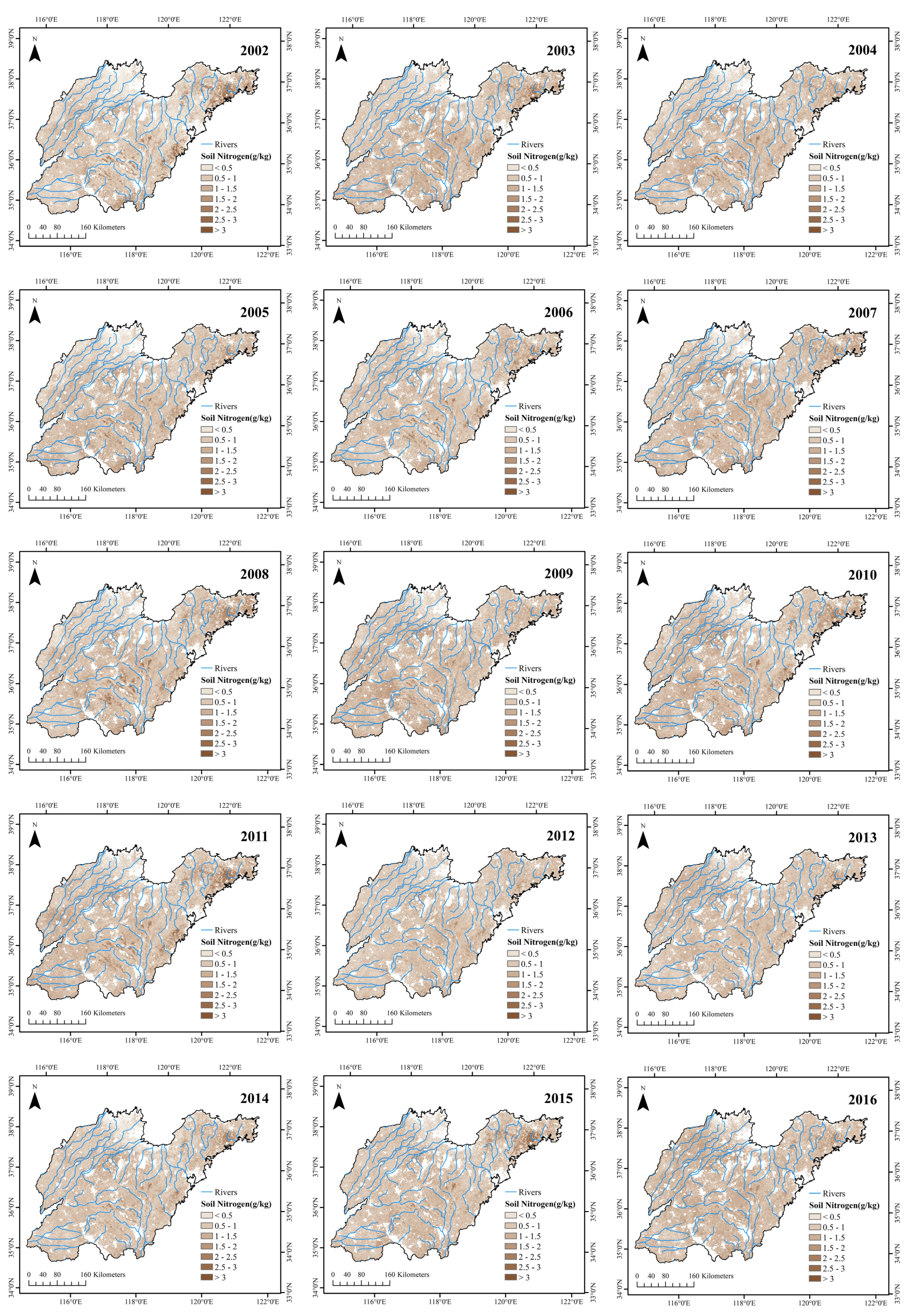
3.3. Spatio-Temporal Characteristics of STN Predictions

We used the RF model to predict the spatial distribution of the STN content in the cropland in Shandong Province from 2002 to 2016 (Figure 6). The STN content changed dynamically with strong spatial distribution differences each year. From the predicted STN content in 2016, the STN distribution seems to have a large overall regional heterogeneity. The mountainous regions had a higher predicted nitrogen content in the northeast followed by the hilly areas in the middle. Low STN contents were found primarily in the western and southern inland regions, and the predicted STN content was relatively low in the southeast coastline regions.
Figure 7 shows variations of the STN content in Shandong Province. The STN content has a stable growth rate with its highest value in 2016 at 1.14 g/kg. Without extreme statistical data, the STN content fluctuated. There was a significant increase from 2002 to 2010, while a downward trend showed up from 2011 to 2015. The predicted STN content fluctuated with an increasing trend from 0.84 g/kg in 2002 to 1.14 g/kg in 2016. Since the regional standard deviation decreased from 0.47 to 0.34 g/kg, the spatial distribution of nitrogen tended to be balanced.
The maps of the STN content predictions from 2002 to 2016 demonstrate that the STN content in most regions increased with a downward trend in the southwest and eastern coastal areas in Shandong Province (Figure 8). The predicted nitrogen content in the northwestern and eastern plains increased significantly. For example, the STN content in Zone A in the northwest plain increased from 0.63 to 1.45 g/kg. The predicted STN content in the southern plain area and the eastern coastline areas decreased; Zone B declined from 1.76 to 1.26 g/kg. The nitrogen content distribution in the remaining areas remained relatively stable within the range of 1.25–1.36 g/kg, such as Zone C.

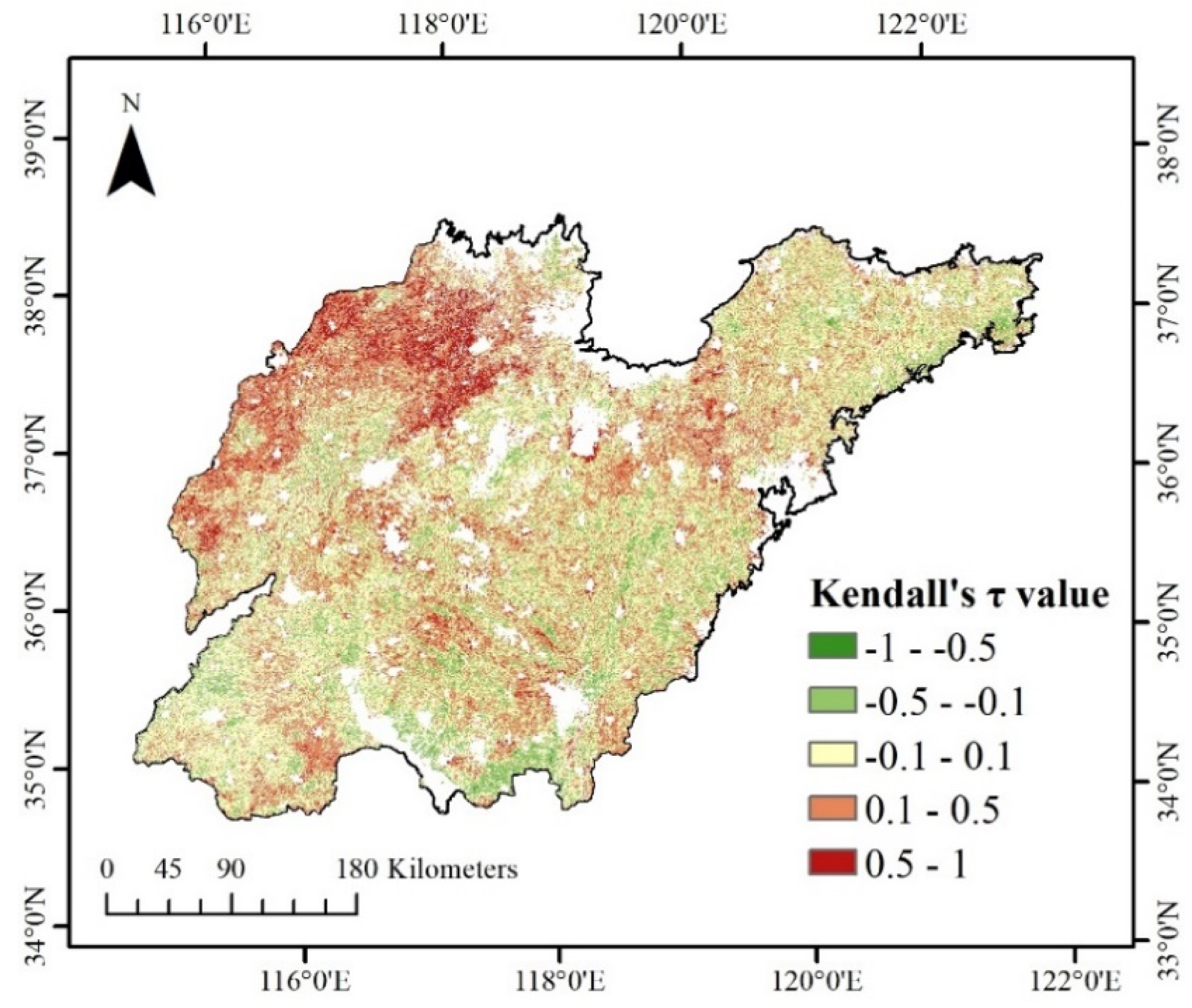
3.4. Spatio-Temporal Trend of STN Predictions

Based on the predicted annual STN spatial distribution from 2002 to 2016, we conducted the Mann–Kendall confidence test at 500 m resolution to evaluate the magnitude of the variation trend, which can distinguish between the rising and falling trend of the areas. Used Theil–Sen Slope estimator to analyze the strength of the spatio-temporal variation trend, so that we can analyze the heterogeneity of the regional STN changing trends.
According to the results of the Mann–Kendall trend test, under the significance level of 95% or higher, the regions present a growth trend of STN which accounts for 64.7% in Shandong Province, mainly concentrated in the northwest plain area. There are also some areas in the eastern plain with an increasing trend of STN. The area showing an STN decline trend accounts for 35.3% and is mainly distributed along the eastern coastline and also in the southern mountainous areas. We regarded the region with the Kendall values in the range from −0.1 to 0.1 as the STN relatively unchanged region. It was found that the regions in which STN remained relatively stable mainly distributed in the southwest and northeast plains of Shandong Province (Figure 9).
Theil–Sen’s slope estimator can estimate the magnitude of the change. It can be seen that the variation range of STN is within the range from −0.17 to 0.23, where the median is 0.01. Among them, it is in relatively 80% of the region that the variation intensity of the STN is not drastic, ranging from −0.03 to 0.03. The area with the largest positive slope is centrally distributed in the northwest of Shandong province. The area with the largest negative slope is in the southeast and the east coast, which is small and scattered. (Figure 10).

4. Discussion

4.1. Predictor Variables Importance

This study used a large amount of remote sensing image data and derivative indices as predictors, including terrain, climate, and other environmental factors, to predict the temporal and spatial distributions of the STN content in Shandong Province. Our study showed that B6_max, B6_mean, B5_mean and B7_mean are the most important predictors to explain the distribution of nitrogen in soils [36,38]. B6_max and B6_mean were calculated from MODIS short-wave infrared (SWIR) spectroscopy. SWIR wavelength range has a significant correlation with STN, which contains the absorption peaks of N-H chemical bonds in proteins [72]. Water has strong absorption characteristics in the SWIR region; thus, this band can provide relevant information to soil moisture [73]. Xu et al. [37] showed that soil moisture is an important predictor variable that is strongly correlated with the nitrogen content based on the at-satellite brightness temperature spectrum data. B5_mean was derived from MODIS mid-infrared (MIR) spectroscopy. MIR spectroscopy is often used to predict soil properties [74]. Near-infrared (NIR) spectroscopy proved to be related to soil nitrogen directly and can independently predict the spatial distribution of soil nitrogen content, which can be seen in previous studies [75]. Remote sensing reflectance plays an important role in STN predictions [76]. VIS-NIR-SWIR and other remote sensing images have been gradually used to predict STN [77] and other soil properties [78]. The vegetation index plays an important role in soil properties prediction. NDWI is a vegetation index that characterizes the liquid water content in vegetation and it was calculated from MIR spectroscopy data only in the MODIS products. The visible blue and green bands are the important predictors for the distribution of STN, and their reflection bands are closely related to the vegetation cover [35,36]. Previous studies have shown that vegetation cover can affect nitrogen accumulation which is highly correlated with the STN content [79]. Besides, other environmental variables also show robust performances in the estimation of the STN content, such as precipitation and elevation, which can play important roles in the spatial pattern of the STN content at regional scales.

4.2. Spatial and Temporal Changes in Predicted STN

The distribution of the STN content has a significant spatial heterogeneity, which is strongly connected with the local environment. The STN content in plain areas is lower than in mountainous areas, which is consistent with previous studies [9,41,65]. The regions with striped high-nitrogen content distribution along the mountains are affected by the altitude in the central and northern part of Shandong Province. Water plays an important role in retaining the STN content. Previous studies have shown that soil with greater water content can promote soil nitrogen accumulation, which explains the high soil nitrogen content in the Yellow River Delta region [44,61]. Soils with a high moisture content can store more nitrogen, which leads to higher STN contents in coastal or wetland regions.
In addition to the influence of natural conditions, changes in the STN content are closely related to human activities. The overall STN content in Shandong Province shows a fluctuating trend, which may be due to the application of fertilizers. Plains are the major terrain in Shandong Province, and the application of fertilizers in intensive agricultural production may lead to an increased STN content. In the northwestern part of Shandong Province, the STN content showed a significant increasing trend. The flat and inland northwestern region with high land productivity [80], which is covered with a network of waterways, is suitable for crop planting. To increase yield, the long-term application of fertilizers is inevitable. Such human activities will affect the mineralization of soil nitrogen and change the spatial distribution of the nitrogen content [81]. In previous studies, spatial and temporal changes in the STN also showed similar increasing trends around the Poyang Lake area and in Jiangxi Province due to the application of nitrogen fertilizers [79,82]. Based on the data of fertilizer application from China’s National Statistics Yearbook [52], the amount of nitrogen fertilizer used in Shandong Province was reduced from 1.97 to 1.51 million tons, and the manure increased from 4.29 to 4.64 million tons from 2002 to 2016, which is a significant increase of 8.14%. The increased STN is not only the effect of applied nitrogen fertilizer but the combination of nitrogen fertilizer and manure that retains soil mineral nitrogen [75]. This reduces the mineralization rate and promotes the absorption and utilization of the nitrogen content, thereby increasing the STN content [76]. With continued agricultural development, the application of chemical fertilizers in China is much higher than the world average to ensure sufficient food production. However, the problem of low nitrogen use efficiency in agricultural production leads to the gradual accumulation of nitrogen in the soil [77]. Effective STN content can guarantee agricultural management in response to the shortage of water resources and intensive human activities. Therefore, it is necessary to monitor the nitrogen content of cropland in the long-term to promote sustainable development in agriculture.

4.3. Advantages and Limitations of the Proposed Approach

The RF model was used to analyze the distribution of the STN content at the provincial scale in this study. Due to its higher accuracy and stability, the RF algorithm is the prevailing approach for predictions when there are large amounts of data [83]. Considering the long-term global remote sensing imagery stored on the GEE platform, the MODIS data provide sufficient band reflectance and derivative indices. Remote sensing data reflects important soil information and plays an important role in predicting the spatial distribution of STN. Remote sensing data can determine where lacking in soil sampling data based on the continuity of space, which provides a basis for predicting soil properties [59]. High-speed computations based on the GEE platform provide technical support, which can accelerate the data processing time in the analysis of massive soil properties [49]. We built the RF model to predict the annual spatial distribution of STN in Shandong province from 2002 to 2016 with the support of the GEE platform, which can monitor the change in the spatial distribution of soil property effectively.
However, one of the limitations is that the prediction accuracy of STN is low in our study (R2 = 0.57). Chen et al. [40] used MODIS data (500 m) to predict soil organic matter with an accuracy of 0.61. Xu et al. [24] used Landsat data (30 m) to predict soil total nitrogen and available potassium with an accuracy of 0.65 and 0.50. Zhang et al. [38] used Sentinel-2A data (10 m) to predict soil organic matter with an accuracy of 0.8. The low-resolution remote sensing spectral data limit the prediction accuracy of STN mapping obviously. Meanwhile, it is difficult to achieve high-precision prediction of soil nutrients with low spatial resolution data by adjusting model parameters [84,85]. Random forest plus residuals kriging approach [18] can be introduced to improve the STN prediction model. However, this method will reduce efficiency due to data migration and calculation in different platforms. This study focused on the series change of STN based on the annual monitoring, but not the comparison of methods for better accuracy. The long-term low-resolution remote sensing data can be used to analyze the spatial pattern and variation trend of the surface environment from a regional-scale. Chen et al. [40] proved that the average soil organic matter showed an upward trend in Hubei province farmland by using MODIS data (2000–2017). Chen et al. [86] detected a trend of leaf area index (LAI) to determine that China and India led in the greening of the world using MODIS LAI products (2000–2017). We used 500 m MODIS data from 2002 to 2016 to analyze soil nitrogen content in farmland in Shandong Province, and the results showed that soil nitrogen content was on the rise in this region.
We will further explore the STN mapping method to predict quickly and accurately on the GEE platform. The enhancements can be taken from two aspects of data selection and model improvement in future studies. On the one hand, the high-resolution remote sensing data (such as 10 m Sentinel-2A data) will be used to predict STN in a more accurate way. On the other hand, Different machine learning algorithms can be applied and residual interpolation can be added to improve model performance and select the most appropriate method. Various algorithms can provide more diverse options for spatial predictions, thereby improving the prediction accuracy of DSM and providing technical support for soil management policies.

5. Conclusions

In this study, we used the RF algorithm on the GEE platform to predict and map the spatial distribution of the STN content each year from 2002 to 2016 in Shandong Province, China. Our research found that:
(1) Overall, the average STN content showed a slightly increasing trend from 2002 to 2016. The areas with an increased trend account for 64.7%, which is concentrated primarily in the northwest of the province, while it decreased slightly in the eastern coastal and central hilly areas. The distribution of the STN content tended to be regionally balanced with less differentiation.
(2) The evaluation of the importance of variables showed that SWIR and MIR reflectance (B6_max, B6_mean, B5_mean and B7_mean) are the most important variables when predicting the STN content in Shandong Province, which shows a strong relationship with STN content. NDWI derived from MODIS was also the key factor for the prediction of STN content.
(3) The GEE platform has substantial remote sensing spectral data, which ensures its relative accuracy and can effectively monitor dynamic changes of the STN content. In addition, the high-speed calculation process provides an approach to predict the spatial distribution of soil properties at larger spatial and temporal scales, which significantly improves the efficiency of STN content evaluation and supervision in future long-term field investigations.

Author Contributions

Conceptualization, W.X. and T.H.; methodology, W.X., T.H., W.C.; software, T.H.; validation, T.H.; formal analysis, W.C., J.G.; investigation, L.R.; data curation, T.H., W.C.; writing—original draft preparation, W.C., L.R.; writing—review and editing, W.X., T.H.; visualization, W.C., J.G.; supervision, W.X.; project administration, W.X.; funding acquisition, W.X. All authors have read and agreed to the published version of the manuscript.

Funding

This research was funded by Joint funds of the Humanities and Social Sciences of Ministry of Education Foundation of China (20C10335010), as well as by the National Nature Science Foundation of China (No. 42071250).

Conflicts of Interest

The authors declare no conflict of interest.

References

  1. Vitousek, P.; Howarth, R. Nitrogen limitation on land and in the sea: How can it occur? Biogeochemistry 1991, 13. [Google Scholar] [CrossRef]
  2. Stevens, C.J.; Dise, N.B.; Mountford, J.O.; Gowing, D.J. Impact of nitrogen deposition on the species richness of grasslands. Science 2004, 303, 1876–1879. [Google Scholar] [CrossRef] [PubMed] [Green Version]
  3. Peri, P.L.; Rosas, Y.M.; Ladd, B.; Toledo, S.; Lasagno, R.G.; Martínez Pastur, G. Modeling Soil Nitrogen Content in South Patagonia across a Climate Gradient, Vegetation Type, and Grazing. Sustainability 2019, 11, 2707. [Google Scholar] [CrossRef] [Green Version]
  4. Carpenter, S.R.; Caraco, N.F.; Correll, D.L.; Howarth, R.W.; Sharpley, A.N.; Smith, V.H. Nonpoint pollution of surface waters with phosphorus and nitrogen. Ecol. Appl. 1998, 8, 559–568. [Google Scholar] [CrossRef]
  5. Powlson, D.S.; Gregory, P.J.; Whalley, W.R.; Quinton, J.N.; Hopkins, D.W.; Whitmore, A.P.; Hirsch, P.R.; Goulding, K. Soil management in relation to sustainable agriculture and ecosystem services. Food Policy 2011, 36, S72–S87. [Google Scholar] [CrossRef]
  6. Yan, W.; Jiang, W.; Han, X.; Hua, W.; Yang, J.; Luo, P. Simulating and Predicting Crop Yield and Soil Fertility under Climate Change with Fertilizer Management in Northeast China Based on the Decision Support System for Agrotechnology Transfer Model. Sustainability 2020, 12, 2194. [Google Scholar] [CrossRef] [Green Version]
  7. Huang, J.; Xu, J.; Liu, X.; Liu, J.; Wang, L. Spatial distribution pattern analysis of groundwater nitrate nitrogen pollution in Shandong intensive farming regions of China using neural network method. Math. Comput. Model. 2011, 54, 995–1004. [Google Scholar] [CrossRef]
  8. Chen, Y.; William, R.W.; Anna, L.H.; Eve-Lyn, S.H. The role of physical properties in controlling soil nitrogen cycling across a tundra-forest ecotone of the Colorado Rocky Mountains, U.S.A. CATENA 2020, 186, 104369. [Google Scholar] [CrossRef]
  9. BATJES, N.H. Total carbon and nitrogen in the soils of the world. Eur. J. Soil Sci. 1996, 47, 151–163. [Google Scholar] [CrossRef]
  10. Robinson, T.P.; Metternicht, G. Testing the performance of spatial interpolation techniques for mapping soil properties. Comput. Electron. Agric. 2006, 50, 97–108. [Google Scholar] [CrossRef]
  11. McBratney, A.; Mendonça Santos, M.; Minasny, B. On digital soil mapping. Geoderma 2003, 117, 3–52. [Google Scholar] [CrossRef]
  12. Elbasiouny, H.; Abowaly, M.; Abu_Alkheir, A.; Gad, A. Spatial variation of soil carbon and nitrogen pools by using ordinary Kriging method in an area of north Nile Delta, Egypt. CATENA 2014, 113, 70–78. [Google Scholar] [CrossRef]
  13. Wang, K.; Zhang, C.; Li, W. Predictive mapping of soil total nitrogen at a regional scale: A comparison between geographically weighted regression and cokriging. Appl. Geogr. 2013, 42, 73–85. [Google Scholar] [CrossRef]
  14. Morellos, A.; Pantazi, X.-E.; Moshou, D.; Alexandridis, T.; Whetton, R.; Tziotzios, G.; Wiebensohn, J.; Bill, R.; Mouazen, A.M. Machine learning based prediction of soil total nitrogen, organic carbon and moisture content by using VIS-NIR spectroscopy. Biosyst. Eng. 2016, 152, 104–116. [Google Scholar] [CrossRef] [Green Version]
  15. Sorenson, P.T.; Quideau, S.A.; Rivard, B.; Dyck, M. Distribution mapping of soil profile carbon and nitrogen with laboratory imaging spectroscopy. Geoderma 2020, 359, 113982. [Google Scholar] [CrossRef]
  16. Hamzehpour, N.; Shafizadeh-Moghadam, H.; Valavi, R. Exploring the driving forces and digital mapping of soil organic carbon using remote sensing and soil texture. CATENA 2019, 182, 104141. [Google Scholar] [CrossRef]
  17. Keshavarzi, A.; Sarmadian, F.; Omran, E.-S.E.; Iqbal, M. A neural network model for estimating soil phosphorus using terrain analysis. Egypt. J. Remote Sens. Space Sci. 2015, 18, 127–135. [Google Scholar] [CrossRef] [Green Version]
  18. Hengl, T.; Heuvelink, G.B.M.; Kempen, B.; Leenaars, J.G.B.; Walsh, M.G.; Shepherd, K.D.; Sila, A.; MacMillan, R.A.; Mendes de Jesus, J.; Tamene, L.; et al. Mapping Soil Properties of Africa at 250 m Resolution: Random Forests Significantly Improve Current Predictions. PLoS ONE 2015, 10, e0125814. [Google Scholar] [CrossRef]
  19. Adhikari, K.; Kheir, R.B.; Greve, M.B.; Bøcher, P.K.; Malone, B.P.; Minasny, B.; McBratney, A.B.; Greve, M.H. High-Resolution 3-D Mapping of Soil Texture in Denmark. Soil Sci. Soc. Am. J. 2013, 77, 860–876. [Google Scholar] [CrossRef]
  20. Shi, T.; Cui, L.; Wang, J.; Fei, T.; Chen, Y.; Wu, G. Comparison of multivariate methods for estimating soil total nitrogen with visible/near-infrared spectroscopy. Plant Soil 2013, 366, 363–375. [Google Scholar] [CrossRef]
  21. Liu, S.; Yang, Y.; Shen, H.; Hu, H.; Zhao, X.; Li, H.; Liu, T.; Fang, J. No significant changes in topsoil carbon in the grasslands of northern China between the 1980s and 2000s. Sci. Total Environ. 2018, 624, 1478–1487. [Google Scholar] [CrossRef] [PubMed]
  22. Xu, Y.; Wang, L.; Ma, Z.; Li, B.; Bartels, R.; Liu, C.; Zhang, X.; Dong, J. Spatially Explicit Model for Statistical Downscaling of Satellite Passive Microwave Soil Moisture. IEEE Trans. Geosci. Remote Sens. 2020, 58, 1182–1191. [Google Scholar] [CrossRef]
  23. Clewley, D.; Whitcomb, J.B.; Akbar, R.; Silva, A.R.; Berg, A.; Adams, J.R.; Caldwell, T.; Entekhabi, D.; Moghaddam, M. A Method for Upscaling In Situ Soil Moisture Measurements to Satellite Footprint Scale Using Random Forests. IEEE J. Sel. Top. Appl. Earth Obs. Remote Sens. 2017, 10, 2663–2673. [Google Scholar] [CrossRef]
  24. Dong, W.; Wu, T.; Luo, J.; Sun, Y.; Xia, L. Land parcel-based digital soil mapping of soil nutrient properties in an alluvial-diluvia plain agricultural area in China. Geoderma 2019, 340, 234–248. [Google Scholar] [CrossRef]
  25. Song, Y.-Q.; Zhao, X.; Su, H.-Y.; Li, B.; Hu, Y.-M.; Cui, X.-S. Predicting Spatial Variations in Soil Nutrients with Hyperspectral Remote Sensing at Regional Scale. Sensors 2018, 18, 3086. [Google Scholar] [CrossRef] [Green Version]
  26. Ließ, M.; Glaser, B.; Huwe, B. Uncertainty in the spatial prediction of soil texture. Geoderma 2012, 170, 70–79. [Google Scholar] [CrossRef]
  27. Heil, J.; Michaelis, X.; Marschner, B.; Stumpe, B. The power of Random Forest for the identification and quantification of technogenic substrates in urban soils on the basis of DRIFT spectra. Environ. Pollut. 2017, 230, 574–583. [Google Scholar] [CrossRef] [PubMed]
  28. de Santana, F.B.; de Souza, A.M.; Poppi, R.J. Visible and near infrared spectroscopy coupled to random forest to quantify some soil quality parameters. Spectrochim. Acta A Mol. Biomol. Spectrosc. 2018, 191, 454–462. [Google Scholar] [CrossRef]
  29. Camera, C.; Zomeni, Z.; Noller, J.S.; Zissimos, A.M.; Christoforou, I.C.; Bruggeman, A. A high resolution map of soil types and physical properties for Cyprus: A digital soil mapping optimization. Geoderma 2017, 285, 35–49. [Google Scholar] [CrossRef]
  30. Assami, T.; Hamdi-Aїssa, B. Digital mapping of soil classes in Algeria—A comparison of methods. Geoderma Reg. 2019, 16, e00215. [Google Scholar] [CrossRef]
  31. Forkuor, G.; Hounkpatin, O.K.L.; Welp, G.; Thiel, M. High Resolution Mapping of Soil Properties Using Remote Sensing Variables in South-Western Burkina Faso: A Comparison of Machine Learning and Multiple Linear Regression Models. PLoS ONE 2017, 12, e0170478. [Google Scholar] [CrossRef] [PubMed]
  32. Belgiu, M.; Drăguţ, L. Random forest in remote sensing: A review of applications and future directions. ISPRS J. Photogramm. Remote Sens. 2016, 114, 24–31. [Google Scholar] [CrossRef]
  33. LAMSAL, S.; BLISS, C.M.; GRAETZ, D.A. Geospatial Mapping of Soil Nitrate-Nitrogen Distribution under a Mixed-Land Use System. Pedosphere 2009, 19, 434–445. [Google Scholar] [CrossRef]
  34. Nouri, H.; Chavoshi Borujeni, S.; Alaghmand, S.; Anderson, S.; Sutton, P.; Parvazian, S.; Beecham, S. Soil Salinity Mapping of Urban Greenery Using Remote Sensing and Proximal Sensing Techniques; The Case of Veale Gardens within the Adelaide Parklands. Sustainability 2018, 10, 2826. [Google Scholar] [CrossRef] [Green Version]
  35. Wang, S.; Zhuang, Q.; Wang, Q.; Jin, X.; Han, C. Mapping stocks of soil organic carbon and soil total nitrogen in Liaoning Province of China. Geoderma 2017, 305, 250–263. [Google Scholar] [CrossRef]
  36. Wang, S.; Jin, X.; Adhikari, K.; Li, W.; Yu, M.; Bian, Z.; Wang, Q. Mapping total soil nitrogen from a site in northeastern China. CATENA 2018, 166, 134–146. [Google Scholar] [CrossRef]
  37. Xu, Y.; Wang, X.; Bai, J.; Wang, D.; Wang, W.; Guan, Y. Estimating the spatial distribution of soil total nitrogen and available potassium in coastal wetland soils in the Yellow River Delta by incorporating multi-source data. Ecol. Indic. 2020, 111, 106002. [Google Scholar] [CrossRef]
  38. Zhang, Y.; Sui, B.; Shen, H.; Ouyang, L. Mapping stocks of soil total nitrogen using remote sensing data: A comparison of random forest models with different predictors. Comput. Electron. Agric. 2019, 160, 23–30. [Google Scholar] [CrossRef]
  39. Deng, X.; Ma, W.; Ren, Z.; Zhang, M.; Grieneisen, M.L.; Chen, X.; Fei, X.; Qin, F.; Zhan, Y.; Lv, X. Spatial and temporal trends of soil total nitrogen and C/N ratio for croplands of East China. Geoderma 2020, 361, 114035. [Google Scholar] [CrossRef]
  40. Chen, D.; Chang, N.; Xiao, J.; Zhou, Q.; Wu, W. Mapping dynamics of soil organic matter in croplands with MODIS data and machine learning algorithms. Sci. Total Environ. 2019, 669, 844–855. [Google Scholar] [CrossRef]
  41. Azzari, G.; Lobell, D.B. Landsat-based classification in the cloud: An opportunity for a paradigm shift in land cover monitoring. Remote Sens. Environ. 2017, 202, 64–74. [Google Scholar] [CrossRef]
  42. Kennedy, R.; Yang, Z.; Gorelick, N.; Braaten, J.; Cavalcante, L.; Cohen, W.; Healey, S. Implementation of the LandTrendr Algorithm on Google Earth Engine. Remote Sens. 2018, 10, 691. [Google Scholar] [CrossRef] [Green Version]
  43. Waller, E.K.; Villarreal, M.L.; Poitras, T.B.; Nauman, T.W.; Duniway, M.C. Landsat time series analysis of fractional plant cover changes on abandoned energy development sites. Int. J. Appl. Earth Obs. Geoinf. 2018, 73, 407–419. [Google Scholar] [CrossRef]
  44. Wu, Q.; Lane, C.R.; Li, X.; Zhao, K.; Zhou, Y.; Clinton, N.; DeVries, B.; Golden, H.E.; Lang, M.W. Integrating LiDAR data and multi-temporal aerial imagery to map wetland inundation dynamics using Google Earth Engine. Remote Sens. Environ. 2019, 228, 1–13. [Google Scholar] [CrossRef] [Green Version]
  45. Jin, Z.; Azzari, G.; You, C.; Di Tommaso, S.; Aston, S.; Burke, M.; Lobell, D.B. Smallholder maize area and yield mapping at national scales with Google Earth Engine. Remote Sens. Environ. 2019, 228, 115–128. [Google Scholar] [CrossRef]
  46. Teluguntla, P.; Thenkabail, P.S.; Oliphant, A.; Xiong, J.; Gumma, M.K.; Congalton, R.G.; Yadav, K.; Huete, A. A 30-m landsat-derived cropland extent product of Australia and China using random forest machine learning algorithm on Google Earth Engine cloud computing platform. ISPRS J. Photogramm. Remote Sens. 2018, 144, 325–340. [Google Scholar] [CrossRef]
  47. Padarian, J.; Minasny, B.; McBratney, A.B. Chile and the Chilean soil grid: A contribution to GlobalSoilMap. Geoderma Reg. 2017, 9, 17–28. [Google Scholar] [CrossRef]
  48. Cao, B.; Domke, G.M.; Russell, M.B.; Walters, B.F. Spatial modeling of litter and soil carbon stocks on forest land in the conterminous United States. Sci. Total Environ. 2019, 654, 94–106. [Google Scholar] [CrossRef]
  49. Ivushkin, K.; Bartholomeus, H.; Bregt, A.K.; Pulatov, A.; Kempen, B.; de Sousa, L. Global mapping of soil salinity change. Remote Sens. Environ. 2019, 231, 111260. [Google Scholar] [CrossRef]
  50. Padarian, J.; Minasny, B.; McBratney, A.B. Using Google’s cloud-based platform for digital soil mapping. Comput. Geosci. 2015, 83, 80–88. [Google Scholar] [CrossRef]
  51. Bureau of Statistics Shandong Province. Statistical Yearbook of Shandong 2019; China Statistics Press: Beijing, China, 2019.
  52. National Bureau of Statistics of China. China Statistical Yearbook 2019; China Statistics Press: Beijing, China, 2019.
  53. National Agro-technical Extension Service Center. The Soil Nutrient Dataset from the Soil Testing and Formulated Fertilization Project (2005–2014); China Agricultural Press: Beijing, China, 2015. [Google Scholar]
  54. Huete, A.; Didan, K.; Miura, T.; Rodriguez, E.; Gao, X.; Ferreira, L. Overview of the radiometric and biophysical performance of the MODIS vegetation indices. Remote Sens. Environ. 2002, 83, 195–213. [Google Scholar] [CrossRef]
  55. Jordan, C.F. Derivation of Leaf-Area Index from Quality of Light on the Forest Floor. Ecology 1969, 50, 663–666. [Google Scholar] [CrossRef]
  56. McGillem, C.; Svedlow, M. Short Papers Optimum Filter for Minimization of Image Registration Error Variance. IEEE Trans. Geosci. Electron. 1977, 15, 257–259. [Google Scholar] [CrossRef]
  57. Qi, J.; Chehbouni, A.; Huete, A.R.; Kerr, Y.H.; Sorooshian, S. A modified soil adjusted vegetation index. Remote Sens. Environ. 1994, 48, 119–126. [Google Scholar] [CrossRef]
  58. Gao, B. NDWI—A normalized difference water index for remote sensing of vegetation liquid water from space. Remote Sens. Environ. 1996, 58, 257–266. [Google Scholar] [CrossRef]
  59. Mulder, V.L.; de Bruin, S.; Schaepman, M.E.; Mayr, T.R. The use of remote sensing in soil and terrain mapping—A review. Geoderma 2011, 162, 1–19. [Google Scholar] [CrossRef]
  60. Yang, R.-M.; Zhang, G.-L.; Liu, F.; Lu, Y.-Y.; Yang, F.; Yang, F.; Yang, M.; Zhao, Y.-G.; Li, D.-C. Comparison of boosted regression tree and random forest models for mapping topsoil organic carbon concentration in an alpine ecosystem. Ecol. Indic. 2016, 60, 870–878. [Google Scholar] [CrossRef]
  61. Xu, Y.; Smith, S.E.; Grunwald, S.; Abd-Elrahman, A.; Wani, S.P.; Nair, V.D. Estimating soil total nitrogen in smallholder farm settings using remote sensing spectral indices and regression kriging. CATENA 2018, 163, 111–122. [Google Scholar] [CrossRef] [Green Version]
  62. Dorji, T.; Odeh, I.O.; Field, D.J.; Baillie, I.C. Digital soil mapping of soil organic carbon stocks under different land use and land cover types in montane ecosystems, Eastern Himalayas. For. Ecol. Manag. 2014, 318, 91–102. [Google Scholar] [CrossRef]
  63. Herbst, M.; Diekkrüger, B.; Vereecken, H. Geostatistical co-regionalization of soil hydraulic properties in a micro-scale catchment using terrain attributes. Geoderma 2006, 132, 206–221. [Google Scholar] [CrossRef]
  64. Zeng, C.; Zhu, A.-X.; Liu, F.; Yang, L.; Rossiter, D.G.; Liu, J.; Wang, D. The impact of rainfall magnitude on the performance of digital soil mapping over low-relief areas using a land surface dynamic feedback method. Ecol. Indic. 2017, 72, 297–309. [Google Scholar] [CrossRef]
  65. Zhong, Q.; Zhang, S.; Chen, H.; Li, T.; Zhang, C.; Xu, X.; Mao, Z.; Gong, G.; Deng, O.; Deng, L.; et al. The influence of climate, topography, parent material and vegetation on soil nitrogen fractions. CATENA 2019, 175, 329–338. [Google Scholar] [CrossRef]
  66. Wang, Y.; Zang, S.; Tian, Y. Mapping paddy rice with the random forest algorithm using MODIS and SMAP time series. Chaos Solitons Fractals 2020, 140, 110116. [Google Scholar] [CrossRef]
  67. Lin, L.I.-K. A Concordance Correlation Coefficient to Evaluate Reproducibility. Biometrics 1989, 45, 255. [Google Scholar] [CrossRef]
  68. Pouladi, N.; Møller, A.B.; Tabatabai, S.; Greve, M.H. Mapping soil organic matter contents at field level with Cubist, Random Forest and kriging. Geoderma 2019, 342, 85–92. [Google Scholar] [CrossRef]
  69. Sen, P.K. Estimates of the Regression Coefficient Based on Kendall’s Tau. J. Am. Stat. Assoc. 1968, 63, 1379–1389. [Google Scholar] [CrossRef]
  70. Theil, H. A Rank-Invariant Method of Linear and Polynomial Regression Analysis. In Henri Theil’s Contributions to Economics and Econometrics; Hallet, A.J.H., Marquez, J., Raj, B., Koerts, J., Eds.; Springer: Dordrecht, The Netherlands, 1992; pp. 345–381. ISBN 978-94-010-5124-8. [Google Scholar]
  71. Mann, H.B. Nonparametric Tests against Trend. Econometrica 1945, 13, 245. [Google Scholar] [CrossRef]
  72. Herrmann, I.; Karnieli, A.; Bonfil, D.J.; Cohen, Y.; Alchanatis, V. SWIR-based spectral indices for assessing nitrogen content in potato fields. Int. J. Remote Sens. 2010, 31, 5127–5143. [Google Scholar] [CrossRef]
  73. van der Meer, F. Analysis of spectral absorption features in hyperspectral imagery. Int. J. Appl. Earth Obs. Geoinf. 2004, 5, 55–68. [Google Scholar] [CrossRef]
  74. Bao, Y.; Meng, X.; Ustin, S.; Wang, X.; Zhang, X.; Liu, H.; Tang, H. Vis-SWIR spectral prediction model for soil organic matter with different grouping strategies. CATENA 2020, 195, 104703. [Google Scholar] [CrossRef]
  75. Chang, C.-W.; Laird, D.A. NEAR-INFRARED REFLECTANCE SPECTROSCOPIC ANALYSIS OF SOIL C AND N. Soil Sci. 2002, 167, 110–116. [Google Scholar] [CrossRef]
  76. Zhang, S.; Yan, L.; Huang, J.; Mu, L.; Huang, Y.; Zhang, X.; Sun, Y. Spatial Heterogeneity of Soil C:N Ratio in a Mollisol Watershed of Northeast China. Land Degrad. Develop. 2016, 27, 295–304. [Google Scholar] [CrossRef]
  77. Li, S.; Ji, W.; Chen, S.; Peng, J.; Zhou, Y.; Shi, Z. Potential of VIS-NIR-SWIR Spectroscopy from the Chinese Soil Spectral Library for Assessment of Nitrogen Fertilization Rates in the Paddy-Rice Region, China. Remote Sens. 2015, 7, 7029–7043. [Google Scholar] [CrossRef] [Green Version]
  78. Tziolas, N.; Tsakiridis, N.; Ben-Dor, E.; Theocharis, J.; Zalidis, G. A memory-based learning approach utilizing combined spectral sources and geographical proximity for improved VIS-NIR-SWIR soil properties estimation. Geoderma 2019, 340, 11–24. [Google Scholar] [CrossRef]
  79. Jiang, Y.; Rao, L.; Sun, K.; Han, Y.; Guo, X. Spatio-temporal distribution of soil nitrogen in Poyang lake ecological economic zone (South-China). Sci. Total Environ. 2018, 626, 235–243. [Google Scholar] [CrossRef] [PubMed]
  80. Deng, X.; Gibson, J.; Wang, P. Management of trade-offs between cultivated land conversions and land productivity in Shandong Province. J. Clean. Prod. 2017, 142, 767–774. [Google Scholar] [CrossRef]
  81. Wang, J.; Zhu, B.; Zhang, J.; Müller, C.; Cai, Z. Mechanisms of soil N dynamics following long-term application of organic fertilizers to subtropical rain-fed purple soil in China. Soil Biol. Biochem. 2015, 91, 222–231. [Google Scholar] [CrossRef]
  82. Liu, X.; Zhang, W.; Zhang, M.; Ficklin, D.L.; Wang, F. Spatio-temporal variations of soil nutrients influenced by an altered land tenure system in China. Geoderma 2009, 152, 23–34. [Google Scholar] [CrossRef]
  83. Li, C.; Wang, J.; Wang, L.; Hu, L.; Gong, P. Comparison of Classification Algorithms and Training Sample Sizes in Urban Land Classification with Landsat Thematic Mapper Imagery. Remote Sens. 2014, 6, 964–983. [Google Scholar] [CrossRef] [Green Version]
  84. Dharumarajan, S.; Hegde, R.; Singh, S.K. Spatial prediction of major soil properties using Random Forest techniques—A case study in semi-arid tropics of South India. Geoderma Reg. 2017, 10, 154–162. [Google Scholar] [CrossRef]
  85. Mansuy, N.; Thiffault, E.; Paré, D.; Bernier, P.; Guindon, L.; Villemaire, P.; Poirier, V.; Beaudoin, A. Digital mapping of soil properties in Canadian managed forests at 250 m of resolution using the k-nearest neighbor method. Geoderma 2014, 235–236, 59–73. [Google Scholar] [CrossRef]
  86. Chen, C.; Park, T.; Wang, X.; Piao, S.; Xu, B.; Chaturvedi, R.K.; Fuchs, R.; Brovkin, V.; Ciais, P.; Fensholt, R.; et al. China and India lead in greening of the world through land-use management. Nat. Sustain. 2019, 2, 122–129. [Google Scholar] [CrossRef] [PubMed]
Figure 1. Location of the study area and soil samples.
Sustainability 12 10274 g001
Figure 2. The annual number of soil samples in 2006–2014.
Sustainability 12 10274 g002
Figure 3. Framework for the soil total nitrogen (STN) content prediction.
Sustainability 12 10274 g003
Figure 4. Relative importance of the predictors. (The length of the bars indicates the relative importance of predictors, the red bars are the predictors that were selected to build the random forest (RF) model).
Sustainability 12 10274 g004
Figure 5. Correlation between observed and predicted values of STN. The linear regression equation and statistical measures (coefficient of determination (R2), mean error (ME), root mean square error (RMSE), and Lin’s concordance correlation coefficient (LCCC)) between observed STN and predicted STN are provided.
Sustainability 12 10274 g005
Figure 6. Distribution of the STN content prediction in Shandong Province from 2002 to 2016.
Sustainability 12 10274 g006
Figure 7. Changes in the predicted STN content in Shandong Province from 2002 to 2016.
Sustainability 12 10274 g007
Figure 8. Spatial changes of the STN content and the typical zone where STN content increases (A), decreases (B), and remains unchanged (C) in Shandong Province from 2002 to 2016.
Sustainability 12 10274 g008
Figure 9. The trend magnitude of STN in Shandong at 95% confidence level, 2002–2016 (value > 0 shows an upward trend, value < 0 shows the downward trend).
Sustainability 12 10274 g009
Figure 10. The trend strength of STN in Shandong at 95% confidence level, 2002–2016. (The absolute value represents the intensity of STN change).
Sustainability 12 10274 g010
Table 1. Variables of STN content predictions.
Predictor VariableData SourceScaleSelected for Model-Building
Mean MODIS red band 1 (B1_mean)MOD09A1.006500 mYes
Maximum MODIS red band 1 (B1_max)MOD09A1.006500 mYes
Mean MODIS near-infrared band 2 (B2_mean)MOD09A1.006500 mYes
Maximum MODIS near-infrared band 2 (B2_max)MOD09A1.006500 mYes
Mean MODIS blue band 3 (B3_mean)MOD09A1.006500 mNo
Maximum MODIS blue band 1 (B3_max)MOD09A1.006500 mYes
Mean MODIS green band 4 (B4_mean)MOD09A1.006500 mNo
Maximum MODIS green band 1 (B4_max)MOD09A1.006500 mYes
Mean MODIS mid-infrared band 5 (B5_mean)MOD09A1.006500 mYes
Maximum MODIS mid-infrared band 5 (B5_max)MOD09A1.006500 mNo
Mean MODIS shortwave infrared1 band 6 (B6_mean)MOD09A1.006500 mYes
Maximum MODIS shortwave infrared 1 band 6 (B6_max)MOD09A1.006500 mYes
Mean MODIS shortwave infrared 2 band 7 (B7_mean)MOD09A1.006500 mYes
Maximum MODIS shortwave infrared 2 band 7 (B7_max)MOD09A1.006500 mYes
Mean normalized difference vegetation index (NDVI_mean)Calculate by Elevation MOD09A1500 mNo
Maximum normalized difference vegetation index (NDVI_max)Calculate by Elevation MOD09A1500 mNo
Mean enhanced vegetation index (EVI_mean)Calculate by Elevation MOD09A1500 mNo
Maximum enhanced vegetation index (EVI_max)Calculate by Elevation MOD09A1500 mNo
Mean ratio vegetation index (RVI_mean)Calculate by Elevation MOD09A1500 mNo
Maximum ratio vegetation index (RVI_max)Calculate by Elevation MOD09A1500 mNo
Mean difference vegetation index (DVI_mean)Calculate by Elevation MOD09A1500 mNo
Maximum difference vegetation index (DVI_max)Calculate by Elevation MOD09A1500 mNo
Mean soil-adjusted vegetation index (SAVI_mean)Calculate by Elevation MOD09A1500 mNo
Maximum soil-adjusted vegetation index (SAVI_max)Calculate by Elevation MOD09A1500 mNo
Mean normalized difference water index (NDWI_mean)Calculate by Elevation MOD09A1500 mYes
Maximum normalized difference water index (NDWI_max)Calculate by Elevation MOD09A1500 mYes
Land surface temperature (LST)http://www.resdc.cn/500 mNo
Mean annual precipitation (MAP)http://www.resdc.cn/500 mYes
Elevation (Elevation)http://www.resdc.cn/90 mYes
Slope (slope)Calculate by Elevation90 mNo
Topographic wetness index (TWI)Calculate by Elevation90 mNo
Aspect (aspect)Calculate by Elevation90 mNo
Publisher’s Note: MDPI stays neutral with regard to jurisdictional claims in published maps and institutional affiliations.

