A Multitier Approach to Estimating the Energy Efficiency of Urban Passenger Mobility

Abstract

As society has experiences new modes of mobility in recent years, cities have planned to increase their energy efficiency as a way of reducing environmental impacts and promoting economic development. However, governments face difficulties in establishing mechanisms to determine the best actions in the management of urban mobility regarding energy efficiency and to elaborate a ranking of cities based on energy efficiency in order to better allocate resources. This is due to the complex nature of obtaining a wide range of activity and energy data from a single municipality, especially in data-scarce regions. This paper develops and applies a model for estimating the energy efficiency of urban mobility that is applicable to different contexts and backgrounds. The main contribution of the article is the use of a multitier approach to compare and adjust outputs, considering different transport configurations and data sets. The results indicate that variations in vehicle occupancy and individual motorized transport rates have a significant impact on energy efficiency, which reached 0.70 passenger-kilometers/MJ in Sorocaba, Brazil. However, as the use of electric vehicles increases in this city, this scenario is expected to change. Additionally, the method has been proven to be an important mechanism for benchmarking purposes and for the decision-making process for transport investments.

1. Introduction

The global urban population has expanded at an accelerated pace over the past century, and it is expected to grow even further in the future. In 1950, 30% of world’s population lived in urban areas, while currently the share is 54% [1,2]. Prospective scenarios estimate that 68% of the world’s population will live in urban areas by 2050 [3]. The urbanization process is even more intense in some regions. For instance, about 80% of the European and North American populations live in urban areas [4,5]. In countries such as Brazil and Argentina this proportion reaches 84% and 92%, respectively [3].

As the spatial pattern continuously changes within a city, the environmental implications of this phenomenon emerge as a fundamental issue for the relevant authorities. Although cities occupy only 2% of the world’s land mass, they account for 67% of global primary energy demand [6] (WEC, 2016), 24% of which is consumed for urban mobility [7]. Consequently, cities are responsible for approximately 70% of the total global carbon dioxide (CO₂) emissions, most of which are emitted by the transport sector [8].

Increasing the energy efficiency (EE) in cities is an energy transition strategy that is commonly announced by government authorities as an alternative to reduce environmental impacts. This implies progressively reducing the energy needed by a transport system to provide the same level of activity in cities. Actions that can improve EE in urban areas include the use of collective high-capacity transport modes (e.g., metro and bus systems), in addition to the adoption of zero-emission technologies (e.g., battery electric vehicles or compressed air vehicles), as well as investments in non-motorized transport and teleactivities. These actions are also in line with the international agenda on energy transition, such as the Sustainable Development Goals (SDGs) established by the 2030 Agenda of the United Nations (UN), along with the Nationally Determined Contributions (NDCs). These agendas affect the overall direction of climate-related targets and policies in cities, especially considering important carbon-emitting sectors, such as transport, industry, and energy supply.

In the meantime, with the advent of smart cities, the efficient use of energy is becoming a competitive advantage for municipalities, facilitating access to green financing for investments in renewable energy projects (e.g., through green bonds and structured green funds) and attracting innovative business models (e.g., e-hailing applications, e-car sharing and private charging stations), various industries, different intellectual capabilities, and research institutions. However, to date, studies that assess the effects of private and public initiatives with urban mobility patterns and the consequences on EE are barely addressed in the literature. Consequently, governments currently face difficulties in establishing a benchmarking environment to assess climate performance and best practices in cities for allocating resources, which can hinder the pace of energy transition. A possible explanation is that urban mobility management programs usually encompass a set of interrelated actions, meaning it is difficult to accurately estimate the specific impact of each measure on EE [9].

To overcome these drawbacks, multisectorial collaborative efforts are required to improve the EE of urban mobility [10]. Improvements in EE lead to reductions in energy consumption, greenhouse gases, pollutants and noise levels. Recognizing that the development of smart cities requires huge investments [11], it would be appropriate for these interventions to enhance EE as much as possible. For this, the initial step required would be to develop a method for estimating the EE of urban mobility considering all of these aspects.

Along these lines, this paper aims to estimate the EE of urban passenger mobility through a comprehensive method that encompasses all modes of transport (including non-motorized), technologies, and fuels. The developed multitier approach is adaptable to different contexts and backgrounds concerning data availability. Thus, it can assist governments in the decision-making process on how to better allocate resources, which are scarce in many economies. The estimation of EE considering non-motorized transport is a complex task but increasingly important as cities progressively invest in last mile integration for passenger transport as a means to improve the efficiency of the system and to reduce atmospheric emissions. The approach is then validated in a large city in an emerging economy, namely Sorocaba, Brazil.

Apart from this introduction, Section 2 summarizes and discusses the main studies for estimating the EE of urban mobility. Section 3 presents the proposed approach and data requirements. In Section 4, the results of the conducted experiment are analyzed. Finally, in Section 5, policy implications and further research directions are discussed.

2. Literature Review

This section presents the results of the literature review, which was conducted with the purpose of answering the following research question: “What is the most appropriate procedure for measuring the EE of urban mobility?” Only studies published in the last ten years that are available in the Web of Science database were considered. According to Mongeon and Paul-Hus (2016) [12], this database has the largest catalogue of indexed journals [12]. The results show a lack of literature on this topic, as no relevant studies with this specific purpose were identified. Therefore, we decided to complement this with a documentary review based on reports from national and international institutions, and papers with any publication date. Thus, 14 studies estimating energy use or carbon emissions within city borders were selected, as summarized in Table 1.

The selected studies analyze cities from China (30%), Europe (20%), Brazil (20%), the United States (10%), and India (10%). The others (10%) assess a hypothetical situation. Regarding the size of these cities, 7% are small (up to 100 thousand inhabitants), 33% are medium-sized (between 100 and 500 thousand inhabitants), 47% are large-sized cities (more than 500 thousand inhabitants), and the remaining 13% are megacities (more than 10 million inhabitants).

All studies consider road transport in calculating the EE. Only Szárz (2011), Saujot and Lefèvre (2016), He et al. (2011), and Menezes et al. (2017) [13,14,15,16] also consider rail or non-motorized transport (walking or cycling). At this point, the lack of studies that assess EE by considering all transport modes becomes evident.

Regarding the methodological approach, 29% of the studies adopt a top-down approach, 64% a bottom-up approach, and 7% adopt both, while aiming to adjust the results. Essentially, top-down and bottom-up approaches are methods used for collecting and processing information. The top-down approach quantifies and identifies the aggregate energy use and carbon emissions, usually using national energy balances and default emission factors. As this approach considers only aggregated data and international emission factors, it is impracticable to conduct accurate assessments based on local technology or activity variations (e.g., vehicle stock or vehicle kilometers traveled—VKT). As pointed out by Pissourios (2014) [17], the use of a top-down approach is a limiting factor in urban analysis, as it results in a lack of perspective on local issues.

In turn, the bottom-up approaches quantify and identify the disaggregated energy use and carbon emissions, considering a broader variety of data in order to comprehend and manage each source of energy [18,19,20]. With this approach, it is possible to conduct in-depth assessments of the main drivers of carbon emissions, as it considers detailed variations in technology and activity, especially when it comes to local emission factors.

To date, there is a limited research body covering estimations of the EE of urban mobility considering all transports modes and energy sources, especially using multiple approaches such as bottom-up and top-down. Only Bose and Srinivasachary (1997) [21] used both approaches simultaneously. Their study estimated the demand for travel based on the number of vehicles, distance traveled, and vehicle occupancy rate using exogenous data.

Szász (1982), He et al. (2011), and Tartakovsky et al. (2013) [13,15,22] estimated energy use from urban passenger mobility by adopting only a bottom-up approach, considering input variables such as the average travel distance, average speed, average occupancy per vehicle, energy consumption by trip, and number of trips by mode of transport. None of these used local data, making it difficult to clearly outline the energy use in urban environments, which is an important activity in urban mobility planning considering zero emissions. Finally, Gerboni et al. (2017) [23] provided some preliminary results for integrated modeling of energy use and transport activity using bottom-up models.

On the other hand, Hillman and Rawaswami (2010) [24] estimated the energy consumption and carbon emissions from passenger transport within city boundaries using a top-down approach. The authors considered local energy balances and international emission factors, which were provided by the Intergovernmental Panel on Climate Change (IPCC). Jiang et al. (2014) [25] also proposed using only a top-down approach to understand the relationship between energy use in passenger mobility and the neighborhood design.

Based on the studies presented in

Table 1. Synthesis of literature review.

Author	Activity	Modes	Approach	Data Base	Case Study	Input	Output
Szász (1982) [13]	Passenger	Road	Bottom-up	-	Hypothetical	Energy consumption: distance traveled; consumption coefficient by kilometer and round hour; average speed and average vehicle occupancy	Energy consumption
Bose and Srinivasachary (1997) [21]	Passenger	Road and Rail	Top-down and Bottom-up	Database (National)	New Delhi (India)	Transport activity by mode; vehicle occupancy; total energy demand by mode of transport and type of energy; energy efficiency by type of vehicle and emission factors	Energy consumption, atmospheric pollutant
Hillman and Rawaswami (2010) [24]	Passenger and freight	Road and Air	Top-down	Origin–destination (OD) matrices, Database (National)	Denver, Portland, Seattle, Minneapolis and Austin (USA)	Regional travel volume per year	Energy consumption, CO2e
He et al. (2011) [15]	Passenger	Road	Bottom-up	OD matrices (Company), Database (Municipal)	Jinan (China)	Modal split; travel distance by mode; vehicle occupancy; EE by mode and emission factor	Energy consumption, CO2e
Tartakovsky et al. (2013) [22]	Passenger	Road	Bottom-up	Survey (Company)	Hypothetical	Fleet; number of passengers; distance and vehicle occupancy	EE, atmospheric pollutant
Giordano et al. (2014) [26]	Passenger	Road	Top-down	Database (Continental)	Barcelona (Spain) and Lugano (Switzerland)	Petrol consumption; distance; % of the mileage traveled on urban roads	Energy consumption, CO2, and atmospheric pollutant
Aggarwal and Jain (2014) [27]	Passenger	Road	Bottom-up	Survey, Database (State)	New Delhi (India)	Travel demand; modal split; distance traveled per vehicle; per mode and per fuel CO2 emission factors	Energy consumption, CO2e
Jiang et al. (2014) [25]	Passenger	Road	Top-down	Database (National)	Barcelona (Spain), Amsterdam (Netherlands), London (UK)	Energy consumption; travel frequency; distance per trip; vehicle occupancy; energy intensity factor; consumption coefficient and energy factor by fuel	EE
Guimarães and Leal Junior (2016) [28]	Passenger	Road and Water	Bottom-up	Research (Company)	Rio de Janeiro (Brazil)	Total passengers transported; distance and EE	Energy consumption, CO2, and atmospheric pollutant
Saujot and Lefèvre (2016) [14]	Passenger	Road and Rail	Top-down	Database (National) and Survey	Grenoble (France)	Transport activity by mode; Energy by source, mode, and emission factor	Energy consumption, CO2e
Yang et al. (2017) [29]	Passenger	Road and Rail	Bottom-up	Survey, Database (National and Municipal)	Beijing (China)	Daily displacement data (time; reason) and attributes of each mode (distance; speed; time)	Transport activity, energy consumption, and CO2
Alonso et al. (2017) [30]	Passenger	Road	Bottom-up	(OD) matrices, Database (Municipal)	Madrid (Spain)	Travel distance; speed and travel time; automotive operating costs and vehicle occupancy.	Energy consumption, CO2, and atmospheric pollutant
Menezes et al. (2017) [16]	Passenger and freight	Road and Rail	Bottom-up	Database (Municipal, State and Federal)	São Paulo (Brazil)	Fleet inventory by type of vehicle and fuel; new registered vehicles; vehicle kilometers traveled; age; fuel economy; average number of passengers, tons transported per mode; fuel prices and taxes; GHG emission factors by type of fuel	Transport activity, energy consumption, CO2e
Gerboni et al. (2017) [23]	Passenger and freight	Road, Rail, Air, and Water	Bottom-up	Database (National forecasting or Regional)	Unspecified city (Italy)	Mobility demand and energy by source and mode	Energy consumption, CO2

, one can conclude that the decision to adopt a specific approach to meet the needs of each region reflects the level of detail of the model and the sensitivity analysis of the results. Consequently, it is reasonable to argue that the effects on EE due to the implementation of an urban mobility action are perceived differently when using a bottom-up or top-down approach. For this reason, we identified the main inputs considered in the selected studies, as presented in

Table 2. Synthesis of the main input variables of the approaches.

Input	Total	Bottom-Up	Top-Down
Number of passengers transported	11	7	4
Modal split (%)	8	5	3
Distance traveled (km)	9	6	3
Energy source	8	8	0
Category of vehicles	7	7	0
Number of trips by mode	6	6	0
Fuel economy (km/L)	5	5	0
Transport activity passenger-kilometers (pass-km)	5	1	4
Vehicle occupancy (pass/vehicle)	5	5	0

, classifying them according to the approach adopted.

Due to the diversity of vehicles and energy sources involved in road transport, an accurate estimation of EE in this mode requires the use of a bottom-up approach with local input variables. However, in 2006 IPCC Guidelines [31] exclusively adopting a bottom-up approach does not ensure the reliability of the estimates. For this, the adoption of both top-down and bottom-up approaches is a fundamental step allowing the comparison and adjustment of results. As evidenced in Table 1, only Bose and Srinivasachary (1997) [21] used more than one approach to estimate the energy use, although the existence of an adjustment protocol is not clearly described on paper.

Furthermore, it is important to state that a bottom-up approach requires a larger amount of data (as shown in Table 2), leading to a complex data collection process. As data availability varies among different economic backgrounds, the use of a bottom-up approach in certain cities may become even more difficult, requiring adaptations from state or national data to represent urban reality, which may compromise the quality of the results. For instance, Bose and Srinivasachary (1997) and Aggarwal and Jain (2014) [21,27] used national data to estimate energy use from urban mobility through a bottom-up approach, while Hillman and Rawaswami (2010), Jiang et al. (2014) and Giordano et al. (2014) [24,25,26] exclusively used national data to represent the same object in a top-down approach.

As a result of the literature review, we also verified that the main tools for estimating energy use in urban mobility are the Long-Range Energy Alternatives Planning system (LEAP) [21], Assessment and Reliability of Transport Emission Models (ARTEMIS) [22], Metropolitan Activity Relocation Simulator (MARS) [30], and For Future Inland Transport Systems (ForFITS) [16]. Most of these tools use a bottom-up approach.

In conclusion, when estimating energy use in urban mobility, the previous research studies did not consider the entire city territory; all transport modes and energy types; or different approaches regarding data availability and adjustment of results. Moreover, none of the methods presented an application. Along these lines, this study considers these literature gaps in developing a method for estimating the EE of urban mobility, which is applied in a large-sized city in a developing country where data availability tends to be scarce.

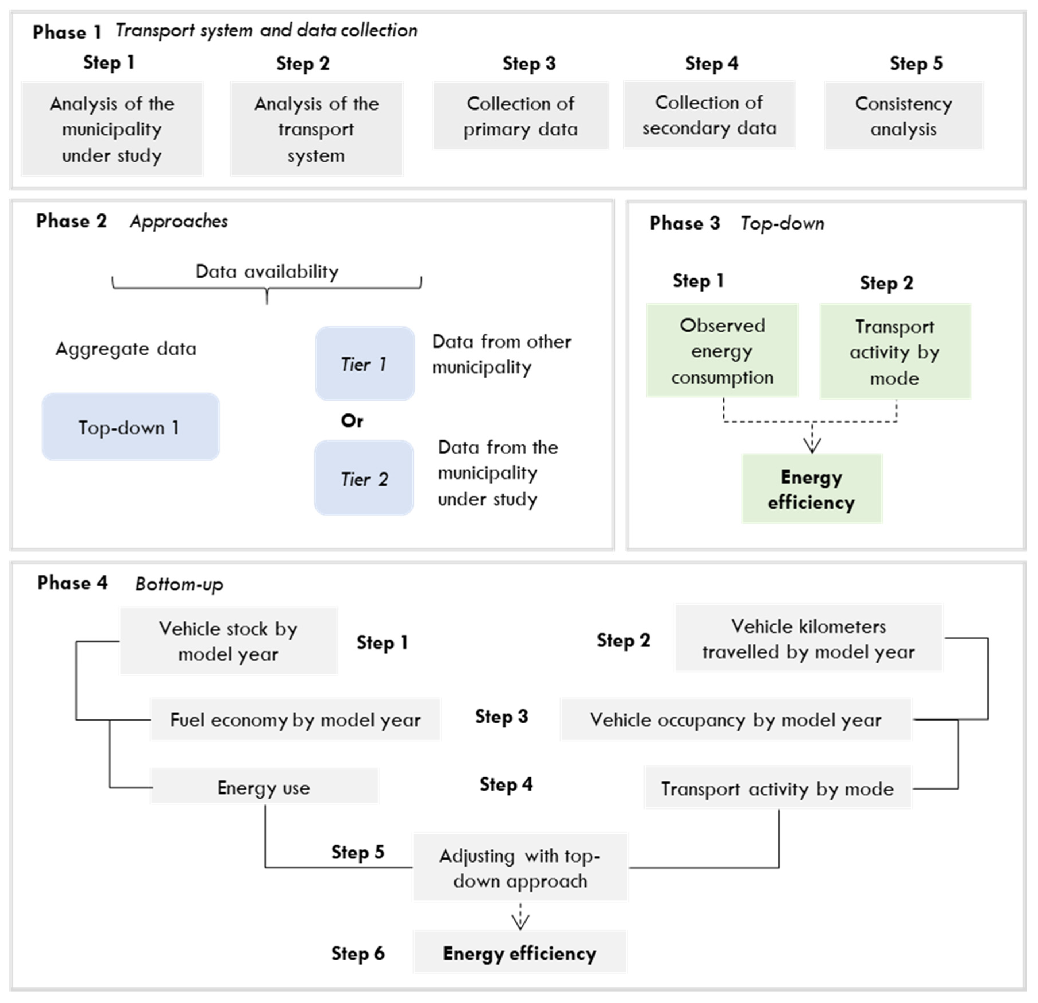
3. Energy Efficiency Model

The energy efficiency model encompasses the road, rail, and water transport modes, including non-motorized transport. Basically, there are two fundamental approaches: top-down and bottom-up. As shown in Figure 1, it is divided into four phases: (1) transport system and data collection; (2) approaches; (3) top-down; (4) bottom-up. The top-down approach is based on aggregated data on energy use and transport activity, while the bottom-up approach is a more detailed mechanism for investigating the effects of several variables on EE.

The bottom-up approach can be divided into two tiers according to data availability: tier 1 and tier 2. In tier 1, data from other municipalities with similar characteristics or from the state or country can be adopted. Consequently, this is used in cases of lack of data or inconsistencies. In turn, tier 2 requires local data from the city being assessed, and thus it provides estimates with greater certainty. However, it is more intensive in collecting and processing information.

The joint use of the two approaches increases accuracy, since EE is estimated through different paths, whereby it is possible to compare and adjust results. In other words, if the same indicator is estimated by two different methods using different data sources and the results are similar, this means that the reliability of this indicator is high. These comparisons and adjustments are particularly desired due to uncertainties related to VKT, fuel consumption, average occupancy, and vehicle stock.

3.1. Data Requirements

Initially, the municipality under study should be described by means of land use, demographic data, transport modes, municipal and inter-municipal fleets, spatial distribution of trips, and transport services (itinerary, demand etc.). Due to the lack of statistics on EE in municipalities and the need to analyze the consistency of the results, we recommend comparing the municipal outputs with those from the state or country (commonly available).

Table 3. Data requirements for each approach.

Inputs	Top-Down	Bottom-Up
		Tier 1	Tier 2
Energy use by source	•	•	•
Modal split	•	•	•
Average trip distance	•	•	•
Fuel economy 1			•
Vehicle stock		•	•
Vehicle kilometers traveled (VKT) 1			•
Average occupancy 1			•

¹ These inputs are also considered in the level 1 approach. However, if they are not available at the local level, assumptions from other cities with similar characteristics can be used or even from the state and the country.

lists the minimum data required to implement each approach considering the selected tier.

It is good practice to compare the outputs (e.g., energy use or transport activity) with macroeconomic data, such as population and gross domestic product (GDP) data, in order to identify inconsistencies. For example, passenger transport activity in municipalities is expected to vary according to GDP per capita. If this relationship is not adherent, the data collected may be inconsistent.

3.2. Top-Down Approach

For rail and water modes, the following inputs are required: energy consumption, total number of passengers transported, and average VKT by trip within city boundaries. The first step consists of estimating the energy use by source. When estimating transport activity (pass-km), it is necessary to obtain the network extension, number of kilometers traveled by line, and number of passengers transported by line (Equation (1)).

$$T{A}_{m,i}^{estimated}={\displaystyle \sum }_l^{⬚}⬚P_l.E_l .M_l$$

(1)

where $T{A}_{m,i}$ is the transport activity by mode (m) in a year (i) (pass-km);$P_l$ is the passengers transported by line (l) (passengers transported by line per year);$E_l$ is the extension of the line (l) (km); $M_l$ is the kilometers traveled per year (i) (%).

Finally, the EE for each mode is estimated by the ratio of the transport activity to energy use (Equation (2)):

$$E{E}_{m,i}=\frac{T{A}_{m,i}}{E{U}_{k,v,i}}$$

(2)

where $T{A}_{m,i}$ is the transport activity by mode (m) in a year (i) (pass-km);$E{U}_{m,i}$ is the energy use by mode (m) in a year (i) (MJ).

For road transport, the aggregate energy consumption by source is required. Usually, such information is available in emission inventories or reports from energy agencies. The next step consists of estimating the transport activity by mode and transport service. This information is generally available in origin–destination (OD) surveys. The EE for road transport is then derived as the ratio of transport activity (pass-km) to energy consumption (MJ).

3.3. Bottom-Up Approach

The bottom-up approach requires disaggregate information on vehicle stock. If such information is not available, it should be estimated considering the number of vehicles sold, a scrappage function, and the average VKT by type of vehicle.

Different approaches can be adopted to estimate the average VKT. Data on bus fleets can be collected directly from local and regional bus companies. For private transport, data can be collected from local interviews, distinguishing commuting, leisure, and intercity trips.

To calculate energy use by source, data on fuel economy by model year is required. Again, for buses, such data can be collected through interviews with local transport operators, while data on private transport can be obtained from manufacturers or reports from sectoral associations.

After estimating the fleet, VKT, and fuel economy by model year, the energy use in urban passenger mobility is estimated through the Equation (3):

$$E{U}_{k,i}^{estimated}=V{S}_{k,i}. F{E}_{k,i}^{ }.VK{T}_{k,i}^{ }$$

(3)

where $E{U}_{k,v,i}$ is the energy use by vehicle type (k) in a year (i) (l or m³);$V{S}_{k,i}$ is the stock of a vehicle type (k) in a year (i) (units)$; F{E}_{k,i}^{ }$ is the fuel economy of a vehicle type (k) in a year (i) (l/km or m³/km);$VK{T}_{k,v,i}$ is the VKT of a vehicle type (k) in a year (i) (km).

Subsequently, Equation (4) presents the calculation used for estimating the transport activity by the model year. The average vehicle occupancy data for buses and private transport vehicles must be collected:

$$T{A}_{k,i}^{estimated}=V{S}_{k,i}. VK{T}_{k,i}^{ } .A{C}_{k,i}^{ }$$

(4)

where $T{A}_{k,i}$ is the transport activity by vehicle type (k) in a year (i) (pass-km); $V{S}_{k,i}$ is the stock of a vehicle type (k) in a year (i) (units);$VK{T}_{k,i}$ is the VKT of a vehicle type (k) in a year (i) (km);$A{C}_{k,i}^{ }$ is the average occupancy of a vehicle type (k) in a year (i) (pass/vehicle).

All energy values are further converted into a common unit (Joules). Then, both energy use and transport activity are compared with the estimates from the top-down approach. Eventual differences are adjusted by changing the VKT or vehicle occupancy values. These modifications should first occur for the parameters with more uncertainty.

It is also important to include active transport. The transport activity from non-motorized trips is the result of multiplying the urban population by the share of pedestrians and cyclists, the frequency of trips, and the average distance by trip. On the other hand, the energy use from non-motorized transport is a result of the transport activity (pass-km) and EE (pass-km/MJ). In Brazil, the reference values for the EE of non-motorized transport are 4.8 pass-km/MJ for walking and 8.9 pass-km/MJ for human-powered bicycles [32].

In summary, the EE for urban mobility is the ratio between the transport activity and energy consumption of all transport modes.

4. Energy Efficiency in Urban Mobility

Sorocaba city was selected as a case study because it was elected to participate in a program by the Ministry of Cities as a model city to receive technical support and public policies focused on energy efficiency. In Brazil, the municipalities must elaborate an Urban Mobility Plan to receive investments in urban mobility, as determined in the National Urban Mobility Policy (NUMP) [33]. Sorocaba was also chosen as the case study due to the existence of urban mobility plans since 2006.

With 644 thousand inhabitants concentrated in 450 km², the city is located 100 km from São Paulo, the richest city in Brazil. The main bases of its economy are the sectors of industry, commerce and services. Trips in Sorocaba are made exclusively by road. The city’s public transport service is offered by two concessionaires, with 261 bus lines, covering an average length of 11.9 km [34,35]. Besides, it has six kilometers of exclusive bus lanes [36].

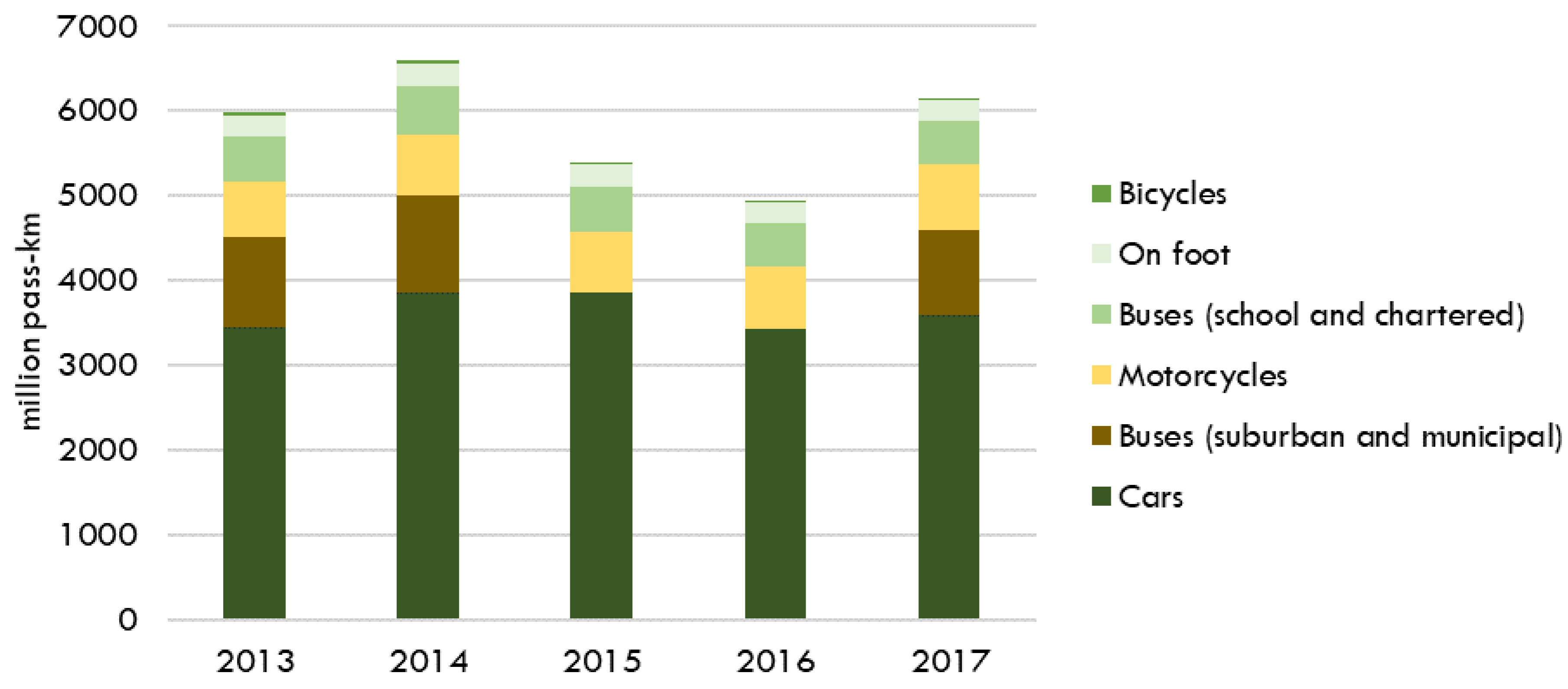
4.1. Aggregate Results

The aggregate fuel consumption data are collected from the Municipal Greenhouse Gas Inventory [37] and ANP (2018) [38]. In Brazil, gasoline is blended with 27% of anhydrous ethanol, while diesel is currently blended with 10% of biodiesel (although this value varied among the time series assessed, from 5% in 2013 to 10% in 2017). Figure 2 shows the fuel consumption from Sorocaba between 2013 and 2017. Since 2015, renewable energy has surpassed fossil fuel energy consumption, accounting for approximately 53% in 2017, mostly from hydrous ethanol use.

From the results presented in the Sorocaba OD Survey, which was conducted in 2013 for 4000 households, it was possible to identify the modal split and average daily travel rate per inhabitant. To project the transport activity, it is also necessary to estimate the average distance traveled per trip and by type of vehicle for each mode of transport. At first, we used a geographic information system (GIS) to produce a cost matrix for each mode of transport (based on the distance traveled), using data from the municipal OD matrix. Nonetheless, the results for buses were not consistent with the data collected directly from the local companies. For this reason, we considered the travel time declared by respondents in the OD survey and the average speed obtained from the Sorocaba Urban and Social Development Company (URBES) (2014) [35] to estimate the average distance per trip by each mode.

Figure 3 presents the transport activity by each type of vehicle and transport mode from 2013 to 2017 using the top-down approach. In view of the information presented in Figure 3, cars (fuel-inefficient vehicles) represent more than the half of the activity in Sorocaba, pointing out the need for actions to promote mobility by bus, bicycle, and foot. This is even more critical when considering that the municipality’s electric car fleet is negligible.

The average EE of urban mobility in Sorocaba using the top-down approach is 0.68 pass-km/MJ. As previously discussed, this value will be used as a reference to adjust the EE estimated by the bottom-up approach.

4.2. Disaggregate Results

The municipal fleet was estimated based on vehicle license statistics obtained from the National Traffic Department and the scrappage curves presented in the study by Gonçalves et al. (2019) [39].

Table 4. Municipal fleet by technology in 2017.

Vehicle	Technology	Stock	Average Age
Cars	Ethanol	1377	15
	NGV	1352	12
	Flexible-fueled 1	150,976	7
	Gasoline	42,084	14
	Hybrid	172	1.4
Light commercials	Flexible-fueled	21,889	7
	Diesel	623	7
	Gasoline	8314	10
Motorcycles	Flexible-fueled	13,117	5
	Gasoline	39,872	9
Micro buses	Diesel	709	6
Buses	Diesel	793	7

¹ Vehicle equipped with an Otto cycle internal combustion engine powered by more than one type of fuel. In Brazil, flexible-fueled vehicles are fueled with gasoline or hydrous ethanol.

shows the vehicle stock in 2017 by model year. This procedure is repeated to estimate the fleet stock by type of vehicle and energy source from 2013 to 2016.

The vehicles with the highest average age are cars with engines that run on ethanol, which are no longer manufactured, followed by gasoline-fueled cars. Hybrid cars have a lower average age as they are still an emerging technology in Brazil.

Table 5. Annual VKT by technology in 2017 (km).

Vehicle	Technology	Annual VKT
Cars	Alcohol	13,595
	Natural Gas Vehicle	13,595
	Flexible-fueled	15,208
	Gasoline	14,309
	Hybrid	15,227
Light commercials	Flexible-fueled	18,255
	Diesel	24,142
	Gasoline	14,624
Motorcycles	Flexible-fueled	13,293
	Gasoline	12,781
Micro buses	Diesel	61,215
Buses		124,735
Buses (school and chartered)		76,880
Articulated buses		42,977

presents the annual VKT by vehicle type. For automobiles, the results were obtained from Goes et al. (2020) and the Environmental Company of the State of São Paulo (CETESB) (2013) [40,41]. For buses, the annual VKT was obtained from surveys conducted with the main companies that operate in Sorocaba. Diesel buses have the largest share due to the intensive use of public transport in the city.

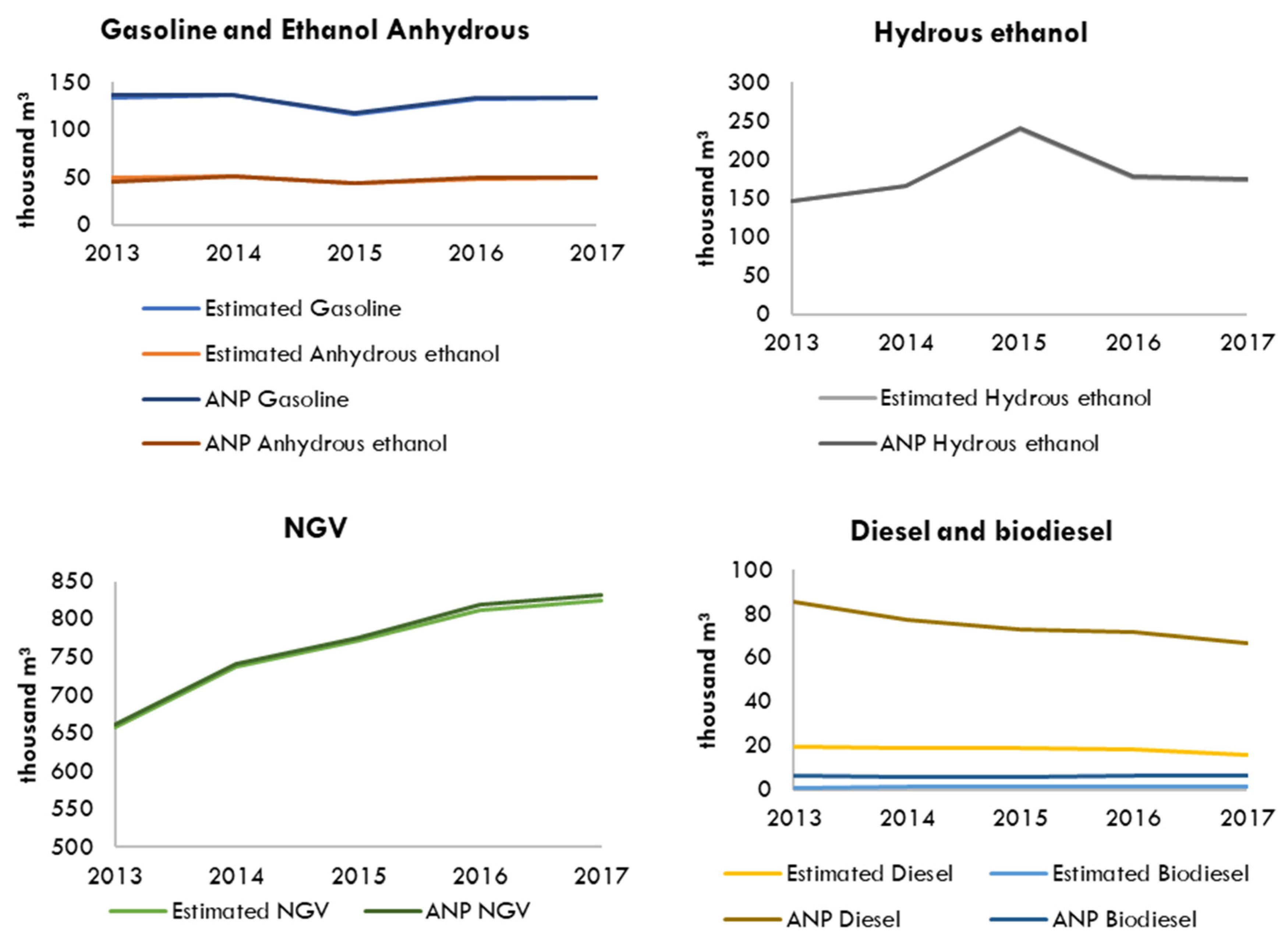
4.2.1. Energy Use by Source

We considered data from the State of São Paulo to estimate the energy use by vehicle [42]. For chartered buses, the fuel economy was obtained through interviews with the main companies that operate in Sorocaba. These buses have the worst fuel economy as compared with other types of vehicles, as shown in

Table 6. Fuel economy per type of vehicle in 2017 (km/l) ¹.

Type of Vehicle	Type of Energy	Fuel Economy (km/L)
Cars	Alcohol	10.9
	Natural Gas Vehicle	12.0
	Flexible-fueled	8.3/12.2
	Gasoline	11.3
	Hybrid	16.5
Light commercials	Flexible-fueled	6.2/8.6
	Diesel	9.5
	Gasoline	11.3
Motorcycles	Flexible-fueled	29.3/43.2
	Gasoline	37.3
Micro buses	Diesel	4.3
Buses		2.9
Buses (school and chartered)		2.6
Articulated buses		1.7

¹ CETESB (2017) [42].

. On the other hand, flexible-fueled and gasoline motorcycles have the best fuel economy.

It is important to state that in Brazil, the number of flexible-fueled vehicles (automobiles fueled by gasoline and hydrous ethanol) is extensive. Therefore, it was necessary to collect historical sales data for Sorocaba to estimate the market share of these fuels in terms of the total energy consumed in flexible-fueled engines. Furthermore, results estimated using the bottom-up approach are adjusted according to the results of the top-down approach, reducing uncertainties. This step is conducted by adjusting the VKT of the different types of vehicles and the share of fuel consumed in flexible-fueled vehicles.

Figure 4 illustrates the baseline energy use by source after the required adjustments, as well as the aggregate fuel consumption values provided by the National Oil Agency (ANP), which were adopted in the top-down approach.

As presented above, both approaches produced similar results from different sources, which indicates methodological maturity in the data collection process. However, this is not the case for diesel, whose fuel consumption data were collected directly from local bus companies, while ANP values represent the total amount consumed by all types of vehicles within the city, such as urban trucks and intercity buses.

To estimate transport activity, the average vehicle occupation rates in the valley and at peak times were collected for each type of vehicle. The average occupancy indicates the number of passengers transported in a vehicle. In the case of urban buses, this value was based on visual surveys conducted during the experiment. For chartered buses, we conducted interviews with the three main companies in Sorocaba, which represent 84% of the city’s fleet. The average occupancy of light vehicles was estimated based on the local OD survey.

Table 7. Occupancy rate per type of vehicle (pass./vehicle).

Type of Vehicle	Average Occupancy 1
Car	1.3
Light commercial	1.0
Motorcycle	1.0
Micro bus	14.5
Basic city bus	32.6
Special and standard buses	44.9
Articulated bus	41.8

¹ Source: Authors, based on the CETESB (2017) and National traffic department (DENATRAN) (2018) [42,43].

summarizes the occupancy rates.

After estimating the fleet, the VKT, and the average occupancy by vehicle, we could estimate the transport activity by mode. Nonetheless, when comparing this value with that estimated using the top-down approach, adjustments were required for the average vehicle occupancy of light vehicles. In this case, differences between both approaches ranges from −0.5% to 2%. For buses, this adjustment was not necessary, as the operational data were collected directly with transport operators.

4.2.2. Energy Efficiency

Table 8. Annual EE and energy intensity values for urban mobility in Sorocaba.

Mode of Transport	2013	2014	2015	2016	2017
On foot	4.81	4.81	4.81	4.81	4.81
Bicycles	8.93	8.93	8.93	8.93	8.93
Motorcycles	1.41	1.37	1.28	1.36	1.45
Cars	0.43	0.48	0.42	0.42	0.44
Buses	2.32	2.32	2.63	2.68	2.89
Bus (suburban and municipal)	2.31	2.39	2.35	2.42	2.54
Total	2013	2014	2015	2016	2017
EE (pass-km/MJ)	0.67	0.72	0.65	0.66	0.70
Energy intensity (kJ/pass-km)	1499	1398	1544	151	1429

shows the annual EE by mode of transport, as well as the resulting average EE and energy intensity values for urban mobility in Sorocaba. These values are also illustrated in Figure 5.

The EE in Sorocaba ranges from 0.67 pass-km/MJ in 2013 to 0.70 pass-km/MJ in 2017. It is important to mention that considering the national perspective, this indicator varied from 0.93 pass-km/MJ to 0.97 pass-km/MJ between 2000 and 2017 in Brazil [44]. Therefore, EE in Sorocaba lies outside this interval. This can be explained by the nature of the input data considered in each case, as the national values also consider long-distance road transport and different modes, such as rail and water, which present higher EE levels.

From this perspective, 44% of the national passenger transport activity is performed by urban buses and 3% by regional buses. In comparison, only 26% of the transport activity in Sorocaba is performed by buses, while 58% of Sorocaba’s transport activity is performed by individual motorized transport (while the national average is 45%). Therefore, Sorocaba’s transport matrix is more dependent on less energy-efficient modes than the national one, thus corroborating the lower EE levels estimated with this method. Additionally, the motorization rate in Sorocaba is higher than the national value at 0.72 vehicles per inhabitant [45] compared to 0.23 vehicles per inhabitant [46], which lowers the estimated EE.

It is also possible to note that the EE values for automobiles vary from 0.42 to 0.48 pass-km/MJ. These values are in accordance with the standards identified in the literature for light passenger vehicles, which vary from 0.33 to 0.59 pass-km/MJ [32,47]. In addition, the estimations over time for EE values for automobiles are the ones that most resemble the average EE in the Sorocaba urban mobility system. This is because automobiles account for 86% of the total energy consumed by the transport sector and approximately 54% of the total transport activity in the city.

Due to historical Brazilian programs aimed at improving vehicular EE, it was expected that these actions would have a more relevant impact on increasing EE in Sorocaba, despite the low average age of the municipality fleet. Even so, the main factor that impacted this indicator in Sorocaba was the average occupancy of vehicles over time.

Finally, it is important to highlight that non-motorized transport contributed to the 4% improvement in the EE of urban mobility. More specifically, these values range from 4.5% (in 2013) to 4.3% (in 2017). Therefore, we reiterate the necessity of considering non-motorized transport when estimating the EE of urban mobility, which is constantly absent in studies on this topic.

5. Conclusions and Policy Implications

This study investigated the relationship between EE and urban mobility to create a benchmarking environment between reference cities related to the energy transition topic. However, the literature review pointed to the lack of specific methods for this purpose. The results suggest the adoption of a bottom-up approach combined with a top-down approach as the most suitable solution for assessing the EE of urban mobility, since it allows data adjustments. This is a fundamental step toward ensuring the accuracy and reliability of the outputs. It is not possible to adjust the results by exclusively adopting a bottom-up approach.

In fact, the adoption of a bottom-up approach using local and disaggregated data is fundamental, especially when considering road transport, due to the diversity of energy sources and vehicles types. Additionally, the level of disaggregation of this approach allows one to measure, evaluate, and report the results through the application of actions that intend to improve the EE of urban mobility. Hence, we recommend simultaneously adopting a bottom-up approach, preferably using a local database, with a top-down approach that considers information from other official data sources at the state or national level and then adjusting eventual divergences.

Along these lines, the model developed to estimate the EE of urban passenger mobility simultaneously considers all of the city territory, transport modes, energy types, and different approaches, depending on data availability. It also addresses the data collection, the steps for which should be carefully followed to guarantee that only transport within city borders is considered when estimating EE.

The method used to estimate the EE of urban mobility was applied to a large city, namely Sorocaba, Brazil. Usually in developing countries such as Brazil, there is a lack of data and statistics on urban mobility. However, the model was successfully applied despite the difficulties faced in the data collection process (e.g., vehicle stock, transport activity, VKT, and occupancy rates). These impedances reinforce the importance of measuring data and statistics on urban mobility. Beyond this, the case study indicated that the method allows adaptations in case of a lack of data, going from a higher level of disaggregation (bottom-up level 2) to a less detailed approach (top-down). The results from this case study confirm the consistency and applicability of the model, since they are within the expected range identified in the national and international literature.

It is important to highlight that the proposed model can be applied by any other city worldwide, as long as the municipality has at least the following data categories available as input variables: energy use by source, modal split, and average trip distance. Although the model has been validated in a Brazilian case study, it can be applied in any other city in the world, as long the necessary data are available. The results can assist municipalities in establishing their baseline for the EE of urban mobility, visualizing the future challenges, and supporting public managers in selecting the most important measures to increase its level of EE and reduce atmospheric emissions.

Furthermore, the application of this method to cities with different characteristics and backgrounds could be the subject of future studies. This would enable benchmarking studies to be developed to determine the best actions for urban mobility management regarding the influence on EE, and even the elaboration of a city ranking based on EE. Additionally, it could also be applied as the basis for the development of an EE standard and certification program for cities. Such a program would recognize participant cities that achieve a minimum level of performance, and specific targets would be set for different levels of ambition.

References

1. World Bank. GINI Index (World Bank Estimate). Available online: https://data.worldbank.org/indicator/SI.POV.GINI?locations=DE-NO-IT (accessed on 19 November 2019).
2. WHO. Health in the Green Economy: Health Co-Benefits of Climate Change Mitigation—Transport Sector; World Health Organization: Geneva, Switzerland, 2011. [Google Scholar]
3. United Nations. 2018 Revision of World Urbanization Prospects. Available online: https://www.un.org/development/desa/publications/2018-revision-of-world-urbanization-prospects.html#:~:text=Today%2C55%25oftheworld’s,increaseto68%25by2050 (accessed on 19 July 2020).
4. Allen, J.; Browne, M. Sustainability strategies for city logistics. In Green Logistics, Improving the Environmental Sustainability of Logistics; McKinnon, A., Browne, M., Whiteing, A., Piecyk, M., Eds.; Kogan Page Limited: London, UK, 2010; pp. 282–305. ISBN 9780749456788. [Google Scholar]
5. United States Census Bureau. 2010 Census Urban and Rural Classification and Urban Area Criteria. Available online: https://www.census.gov/programs-surveys/geography/guidance/geo-areas/urban-rural/2010-urban-rural.html#:~:text=2010CensusUrbanandRuralClassificationandUrbanAreaCriteria,-ComponentID%3A%23ti129393947&text=TheCensusBureauidentifiestwo,andles (accessed on 17 July 2020).
6. Council, W.E. World Energy Scenarios; WEC: London, UK, 2016. [Google Scholar]
7. Millar, D.; Tonolo, G.; Ziebinska, U. Energy Efficiency Indicators: Highlights; IEA: Paris, France, 2016. [Google Scholar]
8. IEA. Cities Are at the Frontline of the Energy Transition. Available online: https://www.iea.org/news/cities-are-at-the-frontline-of-the-energy-transition (accessed on 16 August 2020).
9. Tørnblad, S.H.; Kallbekken, S.; Korneliussen, K.; Mideksa, T.K. Using mobility management to reduce private car use: Results from a natural field experiment in Norway. Transp. Policy 2014, 32, 9–15. [Google Scholar] [CrossRef]
10. EEA. Energy Efficiency and Energy Consumption in the Household Sector 2011; EEA: Copenhagen, Denmark, 2012. [Google Scholar]
11. Mundoli, S.; Unnikrishnan, H.; Nagendra, H. The “Sustainable” in smart cities: Ignoring the importance of urban ecosystems. Decision 2017, 44, 103–120. [Google Scholar] [CrossRef]
12. Mongeon, P.; Paul-Hus, A. The journal coverage of Web of Science and Scopus: A comparative analysis. Scientometrics 2016, 106, 213–228. [Google Scholar] [CrossRef]
13. Szász, P.Á. Eficiência energética do transporte na cidade. Revista dos Transportes Públicos, n. 15. 1982. Available online: http://files-server.antp.org.br/_5dotSystem/download/dcmDocument/2014/08/05/2E97F29A-64FE-4F37-8667-92BE464775E5.pdf (accessed on 31 October 2020).
14. Saujot, M.; Lefèvre, B. The next generation of urban MACCs. Reassessing the cost-effectiveness of urban mitigation options by integrating a systemic approach and social costs. Energy Policy 2016, 92, 124–138. [Google Scholar] [CrossRef]
15. He, D.; Meng, F.; Wang, M.; He, K. Impacts of Urban Transportation Mode Split on CO2 Emissions in Jinan, China. Energies 2011, 4, 685–699. [Google Scholar] [CrossRef] [Green Version]
16. Menezes, E.; Gori-Maia, A.; De Carvalho, C.S. Effectiveness of low-carbon development strategies: Evaluation of policy scenarios for the urban transport sector in a Brazilian megacity. Technol. Forecast. Soc. Chang. 2017, 114, 226–241. [Google Scholar] [CrossRef] [Green Version]
17. Pissourios, I.A. Top-Down and Bottom-Up Urban and Regional Planning: Towards a Framework for The Use of Planning Standards. Eur. Spat. Res. Policy 2014, 21, 83–99. [Google Scholar] [CrossRef]
18. IPCC. Climate Change 2001: The Scientific Basis; IPCC: Cambridge, UK; New York, NY, USA,, 2001. [Google Scholar]
19. Jacobsen, H.K. Integrating the bottom-up and top-down approach to energy–economy modelling: The case of Denmark. Energy Econ. 1998, 20, 443–461. [Google Scholar] [CrossRef] [Green Version]
20. Espinosa, S.I.A. Air Pollution Modeling in São Paulo Using Bottom-Up Vehicular Emissions Inventories; Universidade de São Paulo: São Paulo, Brazil, 2017. [Google Scholar]
21. Bose, R.K.; Srinivasachary, V. Policies to reduce energy use and environmental emissions in the transport sector. Energy Policy 1997, 25, 1137–1150. [Google Scholar] [CrossRef]
22. Tartakovsky, L.; Gutman, M.; Popescu, D.; Shapiro, M. Energy and Environmental Impacts of Urban Buses and Passenger Cars–Comparative Analysis of Sensitivity to Driving Conditions. Environ. Pollut. 2013, 2, 81. [Google Scholar] [CrossRef]
23. Gerboni, R.; Grosso, D.; Carpignano, A.; Chiara, B.D. Linking energy and transport models to support policy making. Energy Policy 2017, 111, 336–345. [Google Scholar] [CrossRef]
24. Hillman, T.; Ramaswami, A. Greenhouse Gas Emission Footprints and Energy Use Benchmarks for Eight U.S. Cities. Environ. Sci. Technol. 2010, 44, 1902–1910. [Google Scholar] [CrossRef]
25. Jiang, Y.; Zegras, P.C.; He, D.; Mao, Q. Does energy follow form? The case of household travel in Jinan, China. Mitig. Adapt. Strat. Glob. Chang. 2014, 20, 701–718. [Google Scholar] [CrossRef]
26. Giordano, P.; Caputo, P.; Vancheri, A. Fuzzy evaluation of heterogeneous quantities: Measuring urban ecological efficiency. Ecol. Model. 2014, 288, 112–126. [Google Scholar] [CrossRef]
27. Aggarwal, P.; Jain, S. Energy demand and CO2 emissions from urban on-road transport in Delhi: Current and future projections under various policy measures. J. Clean. Prod. 2016, 128, 48–61. [Google Scholar] [CrossRef]
28. Guimarães, V.D.A.; Junior, I.C.L. Performance assessment and evaluation method for passenger transportation: A step toward sustainability. J. Clean. Prod. 2017, 142, 297–307. [Google Scholar] [CrossRef]
29. Yang, Y.; Wang, C.; Liu, W.; Zhou, P. Microsimulation of low carbon urban transport policies in Beijing. Energy Policy 2017, 107, 561–572. [Google Scholar] [CrossRef]
30. Alonso, A.; Monzon, A.; Wang, Y. Modelling Land Use and Transport Policies to Measure Their Contribution to Urban Challenges: The Case of Madrid. Sustainability 2017, 9, 378. [Google Scholar] [CrossRef] [Green Version]
31. Intergovernmental Panel on Climate Change. 2006 IPCC Guidelines for National Greenhouse Gas Inventories; Institute for Global Environmental Strategies: Kanagawa, Japan, 2006. [Google Scholar]
32. Marcio de Almeida, D.A. Transportation, Energy Use and Environmental Impacts, 1st ed.; Elsevier: Amsterdam, The Netherlands, 2019; ISBN 978-00120813454-2. [Google Scholar]
33. Brazil Indicadores de Efetividade da Política Nacional de Mobilidade Urbana. Available online: https://www.mdr.gov.br/component/content/article?id=4965 (accessed on 19 July 2020).
34. URBES. Planilhas de Remuneração do Transporte Público. Available online: https://www.urbes.com.br/planilhas-remuneracao (accessed on 19 January 2018).
35. URBES. Plano Diretor de Transporte Urbano e Mobilidade; URBES: Sorocaba, São Paulo, Brazil, 2014. [Google Scholar]
36. URBES. Faixas Exclusivas. Available online: https://www.urbes.com.br/faixas-exclusivas-g/1 (accessed on 19 January 2018).
37. Sorocaba Secretariat of the Environment Inventário de Gases de Efeito Estufa do Município de Sorocaba (2002–2012)—Relatório Final; Sorocaba, Brazil. 2014. Available online: http://sams.iclei.org/novidades/noticias/arquivo-de-noticias/2014/inventario-prefeitura-de-sorocaba.html (accessed on 30 October 2020).
38. ANP RenovaBio. Available online: http://www.anp.gov.br/biocombustiveis/renovabio (accessed on 15 July 2019).
39. Gonçalves, D.N.S.; Goes, G.V.; D’Agosto, M.D.A.; Bandeira, R.A.D.M. Energy use and emissions scenarios for transport to gauge progress toward national commitments. Energy Policy 2019, 135, 110997. [Google Scholar] [CrossRef]
40. Goes, G.V.; Gonçalves, D.N.S.; D’Agosto, M.D.A.; La Rovere, E.L.; Bandeira, R.A.D.M. MRV framework and prospective scenarios to monitor and ratchet up Brazilian transport mitigation targets. Clim. Chang. 2020, 162, 2197–2217. [Google Scholar] [CrossRef]
41. CETESB. Curvas de Intensidade de Uso Por Tipo de Veículo Automotor da Frota da Cidade de São Paulo; CETESB: São Paulo, Brazil, 2013. [Google Scholar]
42. CETESB. Emissões Veiculares no Estado de São Paulo; CETESB: São Paulo, Brazil, 2017. [Google Scholar]
43. DENATRAN. Frota Nacional de Veículos por Município e Tipo. Departamento Nacional de Trânsito. Available online: http://www.denatran.gov.br/estatistica/610-frota-2017 (accessed on 19 July 2020).
44. Gonçalves, D.N.S.; de A. D’Agosto, M. Future Prospective Scenarios for the Use of Energy in Transportation in Brazil and Carbon Emissions Business as Usual (BAU) Scenario—2050; Instituto Brasileiro de Transporte Sustentáve: Rio de Janeiro, Brazil, 2017. [Google Scholar]
45. URBES. Evolução da Taxa de Ocupação Veicular na Última Década. Available online: https://www.urbes.com.br/estatistica-apresentacao (accessed on 19 January 2018).
46. EPE Plano Decenal de Expansão de Energia 2029. 2019. Available online: https://www.epe.gov.br/pt/publicacoes-dados-abertos/publicacoes/plano-decenal-de-expansao-de-energia-2029 (accessed on 30 October 2020).
47. Hughes, P. A Framework for Addressing Transport and Climate Change. Planning Reduced Carbon Dioxide Emissions from Transport Sources. Transp. Plan. Syst. 1994, 2, 29–39. [Google Scholar]
Figure 1. Protocol for estimating energy efficiency in urban mobility.
Sustainability 12 10263 g001
Figure 2. Aggregate fuel (NGV means the energy consumed from Natural Gas Vehicles) consumption.
Sustainability 12 10263 g002
Figure 3. Aggregate transport activity.
Sustainability 12 10263 g003
Figure 4. Fuel consumption by source and technical approach (“estimated” represents the results of the bottom-up approach).
Sustainability 12 10263 g004
Figure 5. Energy efficiency (EE) results for Sorocaba from 2013 to 2017.
Sustainability 12 10263 g005