Reliability Optimization of a Railway Network

Abstract

With the increase of the railway operating mileage, the railway network is becoming more and more complicated. We expect to build more railway lines to offer the possibility to offer more high quality service for the passengers, while the investment is often limited. Therefore, it is very important to decide the pairs of cities to add new railway lines under the condition of limited construction investment in order to optimize the railway line network to maximize the reliability of the railway network to deal with the railway passenger transport task under emergency conditions. In this paper, we firstly define the reliability of the railway networks based on probability theory by analyzing three minor cases. Then we construct a reliability optimization model for the railway network to solve the problem, expecting to enhance the railway network with the limited investment. The goal is to make an optimal decision when choosing where to add new railway lines to maximize the reliability of the whole railway network, taking the construction investment as the main constraint, which is turned to the building mileage limit. A computing case is presented based on the railway network of Shandong Province, China. The computing results prove the effectiveness of the model and the efficiency of the algorithm. The approach presented in this paper can provide a reference for the railway investors and builders to make an optimal decision.

1. Introduction

Nowadays, railway transportation needs to become more and more competitive to get a bigger share of the transportation market. To improve the service quality of the railway is an effective method to keep the market share. There are two approaches to improve the service quality. One is to optimize the railway network, such as extending railway operating mileage and improving the signaling systems to provide more service lines for the passengers. The other is to improve the service plan to offer more choices for the passengers when they travel. Obviously, the first approach is the basis of the second one, as it provides the possibility for the railway operators to design the service plan. Therefore, it is essential to analyze the characteristics of the railway line network, which can help us to form the base to do further research in the field of the railway network optimization.

In fact, there are already many characteristics to be studied when we focus the research work on the railway network: average path length, clustering coefficient, degree distribution, and so on. These characteristics all have explicit definitions, on which we can carry out deep research. However, there are also some characteristics that have no explicit definitions, or the experts have not come to an agreement on the definitions. In this paper, we focus on the reliability of the railway network. We try to define the railway network reliability based on probability theory and design an approach to optimize the railway network in the view of improving the connection reliability of it.

2. Related Works

Railway transit network characteristics analysis has attracted much attention in recent years. Lee and Ghosh (2001) introduced an intuitive definition of stability for a railway transit network, which was an algorithm for railway networks under perturbations [1]. Sen et al. (2003) studied the structural properties of the Indian railway network in the light of investigations of the scaling properties of different complex networks, finding that the Indian railway network displayed small-world properties [2]. Seaton and Hackett (2004) calculated the clustering coefficient, path length, and average vertex degree of two urban train line networks and compared them with theoretical predictions for appropriate random bipartite graphs [3]. Chen et al. (2006) designed a simulation method to study the multi-section features of the cross transportation network and presented countermeasures for reducing the sub-rail and the present reductions at Taipei Metro [4]. Li and Cai (2007) presented a detailed, empirical analysis of the statistical properties of the China railway network consisting of 3915 nodes (train stations) and 22,259 edges (railways), finding that China railway network displayed two explicit features, the small-world property and the scale-free distributions of both degrees and weighted degrees [5]. Ghosh et al. (2011) explored the correlations of the amount of traffic with the topology of the network apart from the small-world characteristics and exponential distribution of node-degrees and edge-weights in the Indian railway network [6]. Martí-Henneberg (2013) analyzed the evolution of railways in Europe since 1840 and aimed to provide a better understanding of present infrastructures and future challenges, based on a new GIS dataset [7]. Innocenti et al. (2014) presented a model for the evaluation of wheel and rail profile evolution due to wear specifically developed for complex railway networks, proposing a statistical approach for the railway track description to study complex railway lines in order to achieve general significant accuracy results in a reasonable time [8]. We built the small-world model for train service network and discussed the LB (Liu and Barabási) model’s adaptability in train service network controllability analysis [9]. Yang et al. (2015) studied urban rail transit network robustness and took the Beijing subway system as an example to assess the robustness of a subway network in the face of random failure as well as malicious attacks [10]. Hu et al. (2015) presented an analytical modeling structure for estimating the probability density function of link lifetime under auto-correlated shadow fading environment in HSR networks, based on the discrete-time Markov chain [11]. Wandelt et al. (2017) developed and implemented a methodology to extract the worldwide railway skeleton network from the open data repository OpenStreetMap, where nodes were stations/waypoints and links were weights with information such as spatial distance, gauge, and maximum speed [12]. Zhao et al. (2017) developed an algorithm for operational risk analysis of railway block sections, measuring the negative impacts caused by the entry delay, extension of running time, dwell time, and departure time [13]. Lu (2018) described a resilience approach for rail transit networks under daily operational incidents that explicitly accounted for the impacts of accumulative affected passengers, quantifying the varying resilience of the rail network with time under different incidents [14]. Caset et al. (2018) represented a systematic empirical assessment of all regional express railway stations in terms of transport and land use characteristics, by drawing on the node-place modeling and transit oriented development literature [15]. Alessio et al. (2019) designed a model to find the topological vulnerabilities in rail networks, focusing on the morning commuter hours when the system was under the most demand stress [16]. Cats and Krishnakumari (2020) adopted a complex network theory approach, investigating metropolitan network performances under alternative sequential disruption scenarios corresponding to the successive closure of either stations or track segments [17]. Olentsevich et al. (2020) presented the dynamics of the throughput capacity of the East Siberian Railway and analyzed the indicator under consideration with parallel and non-parallel schedules, which determined the main factors affecting the throughput capacity of railway stations and sections of the East-Siberian Railway and the degree of their significance [18]. Fang et al. (2020) analyzed the risk of the China high-speed railway network under random attacks and spatially localized failure by Monte Carlo simulation [19]. Zhu and Zhang (2019) proposed a new efficient and more precise three-step complex network reliability approximation approach to enhance the reliability of the complex networked system [20]. Gu (2019) constructed a topological networked model to study and analyze the reliability of high-speed railway network with respect to the destruction caused by natural disasters, geological disasters, equipment failure, or man-made disasters based on the complex network theory [21].

There are also some publications on the transit network characteristics analysis on other transit mode, such as the airport network, the road transit network, and the highway transit network. Hossain and Alam (2017) modeled the Australia’s civil domestic airport infrastructure as a network and analyzed the resulting network structure and its features using complex network tool, taking the degree distribution, characteristics path length, clustering coefficient, and centrality into consideration [22]. Daganzo (2010) described the network shape and operating characteristics of a transit network that allowed a transit system to deliver an accessible level competitive with that of the automobile. Additionally, they revealed which network structure and technology (bus, bus rapid transit, or metro) delivered the desired performance with the least cost. Massimiliano (2015) studied the importance of the functional networks, using the data of delay propagation through European airports [23]. Sullivan et al. (2009) did a review of disturbance analysis on the transit network and the methods hired to deal with the problem of isolating links in different ways of the transit network [24]. Tian et al. (2018) investigated 97 large- and medium-sized cities’ passenger transport network in China, constructing three types of network models—bus stop network, bus transit network, and bus line network, then analyzed the structural characteristics of them [25]. Currie and Delbosc (2014) reviewed the performance of Australasian BRT (Bus Rapid Transit) to identify factors that can best improve performance, analyzing both large-scale busways and the cheaper on-street BRT network [26]. Reynaud et al. (2016) investigated the use of system-wide metrics in the context of Montreal’s urban road network and provided a novel method to evaluate the importance of individual links while internalizing the environmental perspective [27]. Doana and Ukkusuria (2015) studied the inefficiency of the transit network by designing a numeric method [28]. Loustau et al. (2010) studied the travel time reliability on a highway network based on the floating car data [29].

Sun et al. (2016) divided three characteristic types of abnormal passenger flow, comprising “missed” passengers who have left the system, passengers who took detours, and passengers who were delayed but continued their journeys. A real-world case study based on the Beijing metro network with the real tap-in and tap-out passenger data was presented to demonstrate the novel approach [30]. Zhang et al. (2011) measured the topological characteristics by using several parameters; meanwhile, the fraction of removed nodes of Shanghai subway network was discussed and compared against that for a random network, and the critical threshold of this fraction was obtained. Two novel parameters called the functionality loss and connectivity of subway lines were proposed for measuring the transport functionality and connectivity of subway lines [31]. Febbraro et al. (2017) used Petri nets to estimate the indirect consequences of accidents in a railway network [32]. Li et al. (2020) explored the generation and propagation of urban rail transit (URT) risks, and predicted the propagation path and law of URT risks, aiming to prevent and control operational accidents [33].

There are some publications on the transit network vulnerability. Jiang et al. (2018) proposed a station-based accessibility approach addressing passenger flow and land use characteristics in rail-transit network vulnerability analysis [34]. Zhong et al. (2018) proposed an indicator to measure the relevance between two links based on comprehensive analysis of the road transportation network topology and Hazmat road transportation risk characteristics [35]. Ouyang et al. (2014) took the Chinese railway system as an example and selected three typical complex network based models, including a purely topological model, purely shortest path model, and weight (link length) based shortest path model, to analyze railway accessibility and flow-based vulnerability and compare their results with those from the real train flow model [36]. Xiao et al. (2018) represented a subway network as a dynamic, directed, and weighted graph. Static and dynamic metrics that can represent vertices’ and edges’ local and global attributes were proposed [37]. Through a detailed analysis of the Beijing subway network, they illustrated that the heterogeneity and vulnerability of Beijing subway network vary over time when passenger flow was taken into consideration. Oliveira et al. (2016) investigated performance attributed to road networks, reliability, and vulnerability, analyzing their similarities as well as differences that justify distinct definitions, based on consolidation of recent studies [38]. Capacity weighted spectral partitioning was proposed by Núñez and Palomares (2014), aiming at developing a methodology for measuring public transport network vulnerability taking the Madrid Metro system as an example [39]. The consequences of a disruption of riding time or the number of missed trips were analyzed for each of the network links with a full scan approach implemented in GIS (Geographic Information Systems). Balijepalli and Oppong (2014) proposed a new vulnerability index considering the serviceability of road links and illustrated its computation, then used the results to outline a traffic diversion plan in the event of flooding in York using traffic network modelling techniques combined with Geographic Information Systems application [40]. Taylor and Susilawati (2012) considered the development of a method for network vulnerability analysis, which considered the socio-economic impacts of network degradation and sought to determine the most critical locations in the network [41]. Jenelius and Mattsson (2012) described practical indicators and algorithms developed for large-scale vulnerability analyses [42]. They analyzed both single link closures and area-covering disruptions and the distribution of impacts among different regions in a case study on the Swedish road transport system. Betweenness centrality and passenger betweenness centrality, number of missed trips, weighted average path length, and weighted global efficiency were analyzed considering relative disruption probability of each line.

All these publications have given us much inspiration when studying the railway network optimization problem. In this paper, we focus on the reliability analysis and optimization of the high-speed railway network. The contents are organized into four more sections. Section 2 introduces definitions of reliability of a railway network and presents a reliability optimization model. Section 3 gives a computing case base on the data of Shandong railway network. Section 4 analyzes the computing results thoroughly and Section 5 draws the conclusion.

3. Definitions of Reliability and Reliability Optimization Model of a Railway Network

Reliability is the ability or possibility of components, products, or systems that perform a specified function without failure for a certain period of time or under certain conditions. It is a concept in the field of automation research. In railway network, many trains run from stations to other stations, so it is very important for us to keep the availability of the railway lines and stations. Railway sections are more fragile than stations. Therefore, we focus on the reliability of the railway sections in this paper. However, how do we measure the reliability of the railway network?

Here we should answer two questions. One is how to evaluate the reachability from a station to another one, which is the key problem we must solve. The other is how to measure the reliability of a whole network. Clearly, it directly relates to the connection probability of the two nodes. Here we firstly present some minor cases to analyze and define the railway network reliability concept.

3.1. Small Cases and the Concept of Reliability

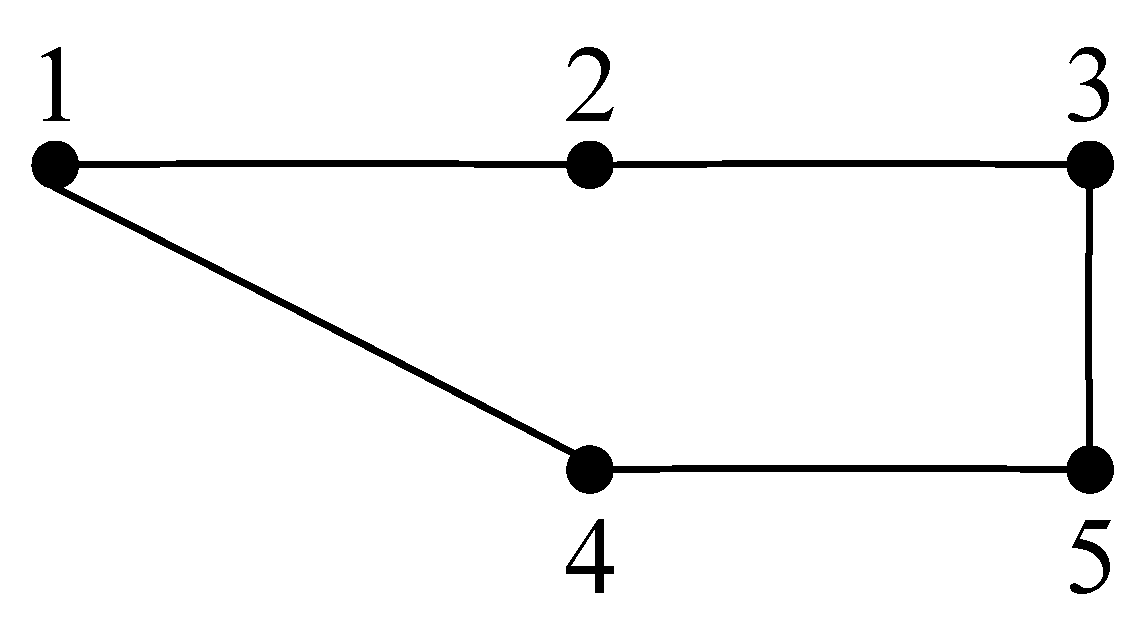
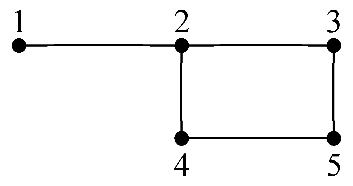
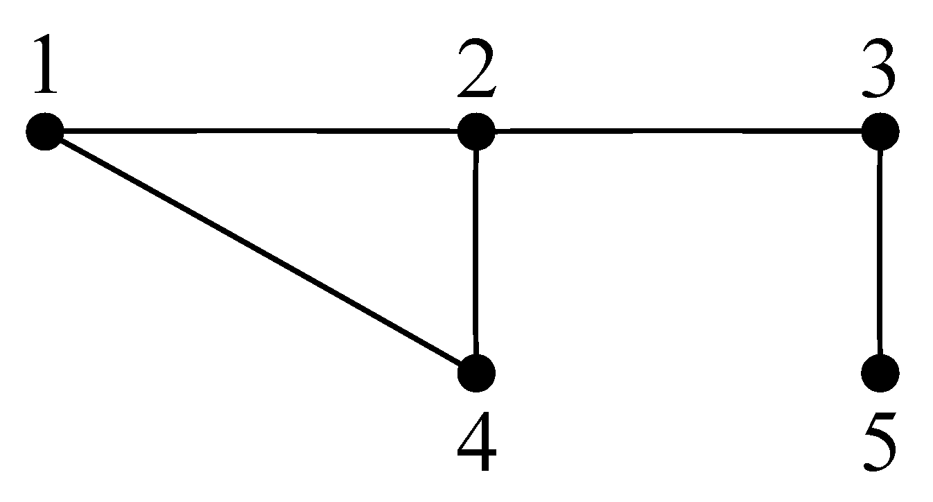
Here we present three small computing cases to illustrate the reliability of a network to make the readers to understand the optimization goal of the problem in this paper. We take it for granted that all of the nodes in the network are available and each pair of nodes is connected with a certain probability, which we assume is 0.8 to explain the calculation method and process.

3.1.1. Case 1

Firstly, we model a railway network with five nodes, forming a ring, which is shown in Figure 1. There are five nodes in Figure 1 which stand for the stations in the railway network, marked with 1, 2, 3, 4, 5. The numbers in Figure 1 are the serial numbers of the nodes in the network.

We calculate the reliability between every pair of nodes in the network in Figure 1. The edges in the network are connected to a ring. Therefore, there are two paths between Node 1 and Node 2. We should consider the reachability comprehensively, taking function of both paths into consideration.

(1) The reliability between Node 1 and Node 2

We can see that there are two paths from Node 1 to Node 2. The first one is 1–2 (marked with p_1–2) and the second one is 1–4–5–3–2 (marked with p_{1–4–5–3–2}). The reachability of p_1–2 equals to the connection probability of e_1–2, which is 0.8, while the reachability of p_{1–4–5–3–2} equals to the product of the connection probability of the edges on the path, which is $0.8\times 0.8\times 0.8\times 0.8=0.4096$.

Then, what is the probability that we can go from Node 1 to Node 2 successfully under this condition? We can check the problem from another perspective. Only if both of the paths are unavailable can we not reach the destination. The probability that we cannot reach Node 2 can be calculated out: $\left(1-0.8\right)\times \left(1-0.4096\right)=0.11808$. Therefore, the probability that we can go from Node 1 to Node 2 is $1-\left(1-0.8\right)\times \left(1-0.4096\right)=0.88192$. For the same reason, the reliability between Node 2 and Node 3, reliability between Node 3 and Node 5, reliability between Node 4 and Node 5, and the reliability between Node 1 and Node 4 are all 0.88192.

(2) The reliability between Node 1 and Node 3

There are two paths between Node 1 and Node 3, as shown in Figure 2. We can see that there are two paths from Node 1 to Node 3, which are 1–2–3 (marked with p_1–2–3) and 1–4–5–3 (marked with p_{1–4–5–3}). The reachability of p_1–2–3 equals to the product of the connection probability of the edges on the path, which is $0.8\times 0.8=0.64$. In the same manner, the reachability of p_{1–4–5–3} is $0.8\times 0.8\times 0.8=0.512$. The probability that we can go from Node 1 to Node 3 is $1-\left(1-0.64\right)\times \left(1-0.512\right)=0.82432$. The reliability between Node 1 and Node 5, between Node 2 and Node 5, between Node 2 and Node 5, and between Node and Node 4 are all 0.82432.

The reliability value between the nodes in Case 1 is shown in

Table 1. Reliability between the nodes in Case 1.

Plan 1	1	2	3	4	5
1	-	0.88192	0.82432	0.88192	0.82432
2		-	0.88192	0.82432	0.82432
3			-	0.82432	0.88192
4				-	0.88192
5					-

.

3.1.2. Case 2

Secondly, we present another case to illustrate the calculation of reliability value between the nodes. We still model a railway network with five nodes, which is shown in Figure 2. There are also five nodes in Figure 2, which stand for the stations in the railway network, marked with 1, 2, 3, 4, and 5. Node 2, Node 3, Node 4, and Node 5 form a ring. The numbers in Figure 2 are the serial numbers of the nodes in the network.

There are also five nodes in the network in Case 2. The topology is shown in Figure 2.

(1) The reliability between Node 1 and Node 2

The reliability between Node 1 and Node 2 is the connection probability between Node 1 and Node 2, which is 0.8 due to the topology in Case 2.

(2) The reliability between Node 2 and Node 3

There are two paths between Node 2 and Node 3. One is 2–3 (marked with p_2–3). The other is 2–4–5–3 (marked with p_{2–4–5–3}). The reachability of p_2–3 is the connection probability of e_2–3, which is 0.8. The reachability of p_{2–4–5–3} equals to the product of the connection probability of the edges on the path, which is $0.8\times 0.8\times 0.8=0.512$. Then the reliability between Node 2 and Node 3 is $1-(1-0.8)\times (1-0.512)=0.9024$. For the same manner, the reliability between Node 2 and Node 4, between Node 3 and Node 5, and between Node 4 and Node 5 are all 0.9024.

(3) The reliability between Node 1 and Node 3

The reliability between Node 1 and Node 2 is the product of reliability between Node 1 and Node 2 and that between Node 2 and Node 3, $0.8\times 0.9042=0.72192$. The reliability between Node 1 and Node 4 equals to the reliability between Node 1 and Node 3.

(4) The reliability between Node 2 and Node 5

There are two paths between Node 2 and Node 5. The reliability between Node 2 and Node 5 is $1-(1-0.64)\times (1-0.64)=0.8704$.

(5) The reliability between Node 1 and Node 5

The reliability between Node 1 and Node 5 is the product of reliability between Node 1 and Node 2 and that between Node 2 and Node 5, $0.8\times 0.8704=0.69632$.

The reliability value between the nodes in Case 2 is shown in

Table 2. Reliability between the nodes in Case 2.

Plan 2	1	2	3	4	5
1	-	0.8	0.72192	0.72192	0.8704
2		-	0.9024	0.9024	0.8704
3			-	0.8704	0.9024
4				-	0.9024
5					-

.

3.1.3. Case 3

Lastly, we present the last case and model a railway network with five nodes, which is shown in Figure 3. There are also five nodes in Figure 3, which stand for the stations in the railway network, marked with 1, 2, 3, 4, and 5. The numbers in Figure 3 are the serial numbers of the nodes in the network.

(1) Reliability between Node 1 and Node 2

We can see that there are two paths in the network in Figure 3. The reachability of p_1–2 is the connection probability of edge e_1–2. The reachability of p_1–4–2 is the product of connection probabilities of edge e_1–4 and edge e_2–4, which is $0.8\times 0.8=0.64$. The reliability is $1-(1-0.8)\times (1-0.64)=0.928$. In the same manner, the reliability between Node 1 and Node 4 and the reliability between Node 2 and Node 4 are both 0.928.

(2) Reliability between Node 1 and Node 3

The reliability between Node and Node 3 is the product of reliability between Node 1 and Node 2 and the reliability between Node 2 and Node 3, which is $0.928\times 0.8=0.7424$. The reliability between Node 4 and Node 3 is the same.

(3) Reliability between Node 1 and Node 5

The reliability between Node 1 and Node 5 depends on the reliability between Node 1 and Node 2, the reliability between Node 2 and Node 3 and the reliability between Node 3 and Node 5. The reliability is $0.928\times 0.8\times 0.8=0.59392$. The reliability between Node 4 and Node 5 is the same.

(4) Reliability between Node 2 and Node 3

The reliability between Node 2 and Node 3 equals to the connection probability edge e_2–3, which is 0.8. The reliability between Node 3 and Node 5 is the same.

(5) Reliability between Node 2 and Node 5

The reliability between Node 2 and Node 5 depends on the reliability between Node 2 and Node 3 and the reliability between Node 3 and Node 5, which is $0.8\times 0.8=0.64$.

The reliability value between the nodes in Case 3 is shown in

Table 3. Reliability between the nodes in Case 3.

Plan 3	1	2	3	4	5
1	-	0.928	0.7424	0.928	0.59392
2		-	0.8	0.928	0.64
3			-	0.7424	0.8
4				-	0.59392
5					-

.

From the three cases above, we can see that there may be more than one path between two nodes. Additionally, the more paths there are between two nodes, the larger the reliability is. We can also conclude that the reliability is connected with the connection probability between the two nodes. To avoid the concept confusion, it is vital for us to give explicit definitions about the reliability in the railway network.

3.2. Definition of Connection Reliability

To determine the optimization goal of the problem, we first present some definitions related to the network reliability based on the small computing cases in Section 3.1.

Definition 1.

Neighboring stations’ direct connection probability: Neighboring stations’ direct connection reliability is the connecting probability of the direct connecting railway sections between the two neighboring stations. We use$p_{i,j}^{NB}$to stand for the neighboring stations’ direct connection probability. The calculation method is shown in Section 3.1.

Definition 2.

Connection reliability between two station nodes on a path: Connection reliability between two station nodes on a path is the connection reliability between two station nodes and the connection probability through a single path, which is determined by the direct connection reliability of the edges on the path.

$$p_{i,j}^P={\displaystyle \prod _{k=i}^{j-1}{p}_{k,k+1}^{NB}}$$

(1)

where$p_{k,k+1}^{NB}$is the neighboring stations’ direct connection reliability between station node k and k + 1.

Definition 3.

Connection reliability between two station nodes: Connection reliability between two station nodes is the comprehensive connecting probability in the railway network, considering all of the available paths between the two stations in the railway network.$p_{i,j}^{CTS}$is used to indicate the connection reliability between Station i and Station j, as shown in Equation (1). The calculation process is shown in Section 3.1 also.

$$p_{i,j}^{CTS}=compose(p_{i,j}^P)$$

(2)

Therefore, we can see that if there is only one path between the two nodes, connection reliability between two station nodes equals to the reachability of the path. However, if there is more than one path between the two nodes, the reliability should be calculated based on the probability theory.

For example, if all of the paths do not have the same edge, the reliability can be defined as

$$p_{i,j}^{CTS}=1-{\displaystyle \prod _{k=1}^{M_{ij}}(1-p_{i,j,k}^P)}$$

(3)

where $M_{ij}$ is the number of paths between Node i and Node j.

If there is at least one shared edge among the paths between two nodes (see Figure 4), the reliability can be defined as

$$p_{i,j}^{CTS}={\displaystyle \prod _{k=i}^{j-1}{p}_{k,k+1}^{CTS}}$$

(4)

However, the topology structure can be more complicated.

Definition 4.

Station node connection reliability: Station node connection reliability is the average connection reliability between the station node and all other station nodes in the railway network. We use$p_i^{CTS}$to indicate the connection reliability of Station i, as shown in Equation (5).

$$p_i^{CTS}=\frac{{\displaystyle \sum _{j=1}^{N-1}{p}_{i,j}^{CTS}}}{N-1},i=1,2,\dots ,N$$

(5)

where N is the number of station nodes in the railway network.

Definition 5.

Railway network connection reliability: Railway network connection reliability is the average connection reliability between all the station nodes in the railway network. We use$p_{}^{NET}$to define the railway network connection reliability, as shown in Equation (6).

$$p_{}^{NET}=\frac{{\displaystyle \sum _{i=1}^N{\displaystyle \sum _{j=1}^{N-1}{p}_{i,j}^{CTS}}}}{N(N-1)/2}=\frac{2{\displaystyle \sum _{i=1}^N{\displaystyle \sum _{j=1}^{N-1}{p}_{i,j}^{CTS}}}}{N(N-1)}$$

(6)

The destination of this paper is to design a method to improve the connection reliability of a railway network. Therefore, we take the railway network connection reliability as the optimization goal.

3.3. Reliability Network Optimization Model Based on Reliability

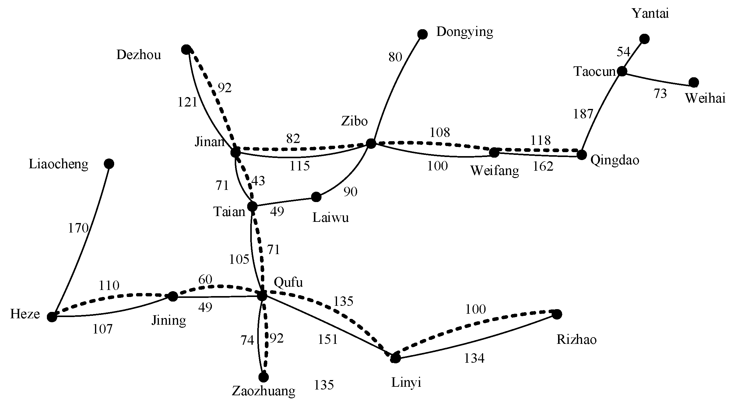
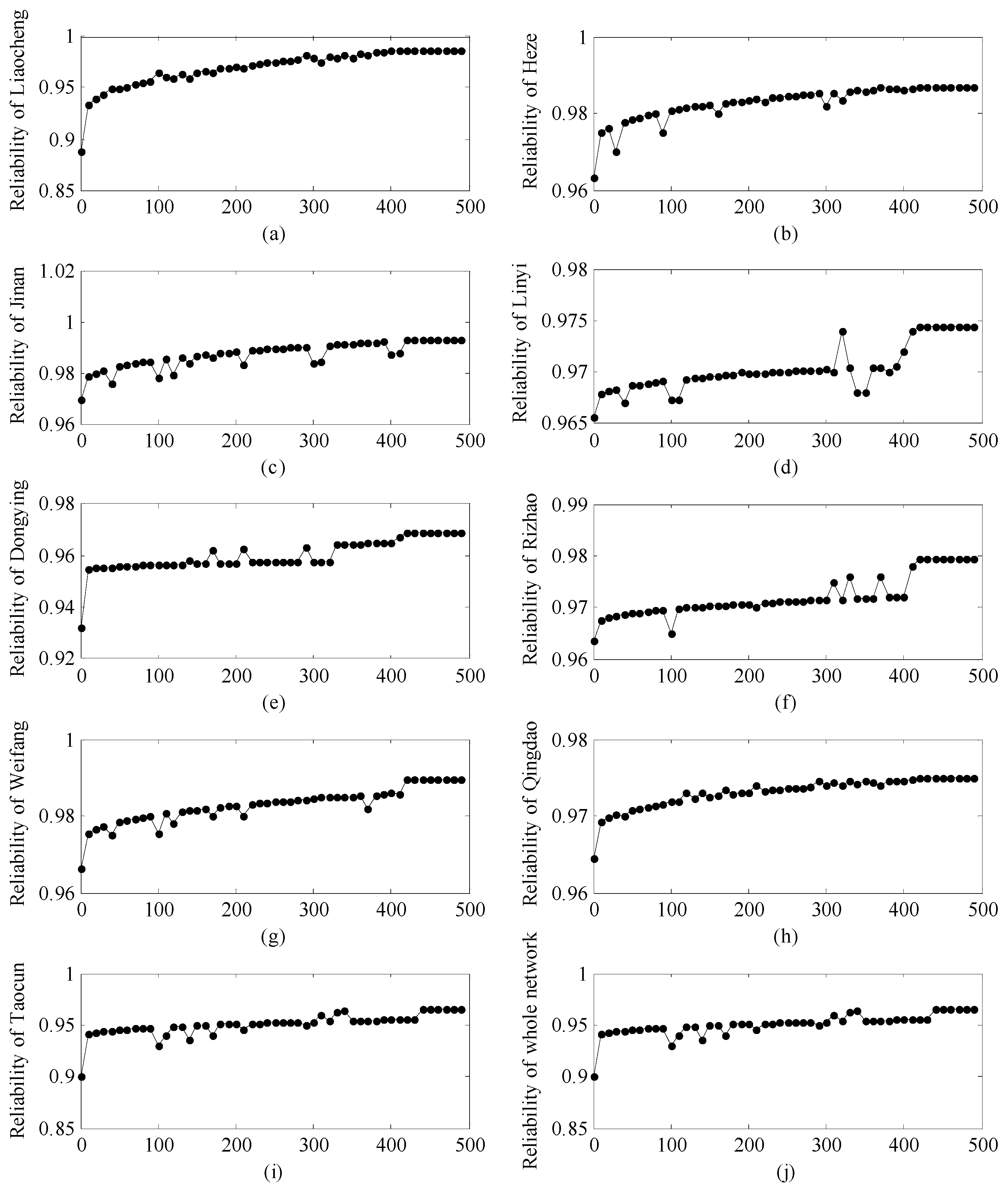
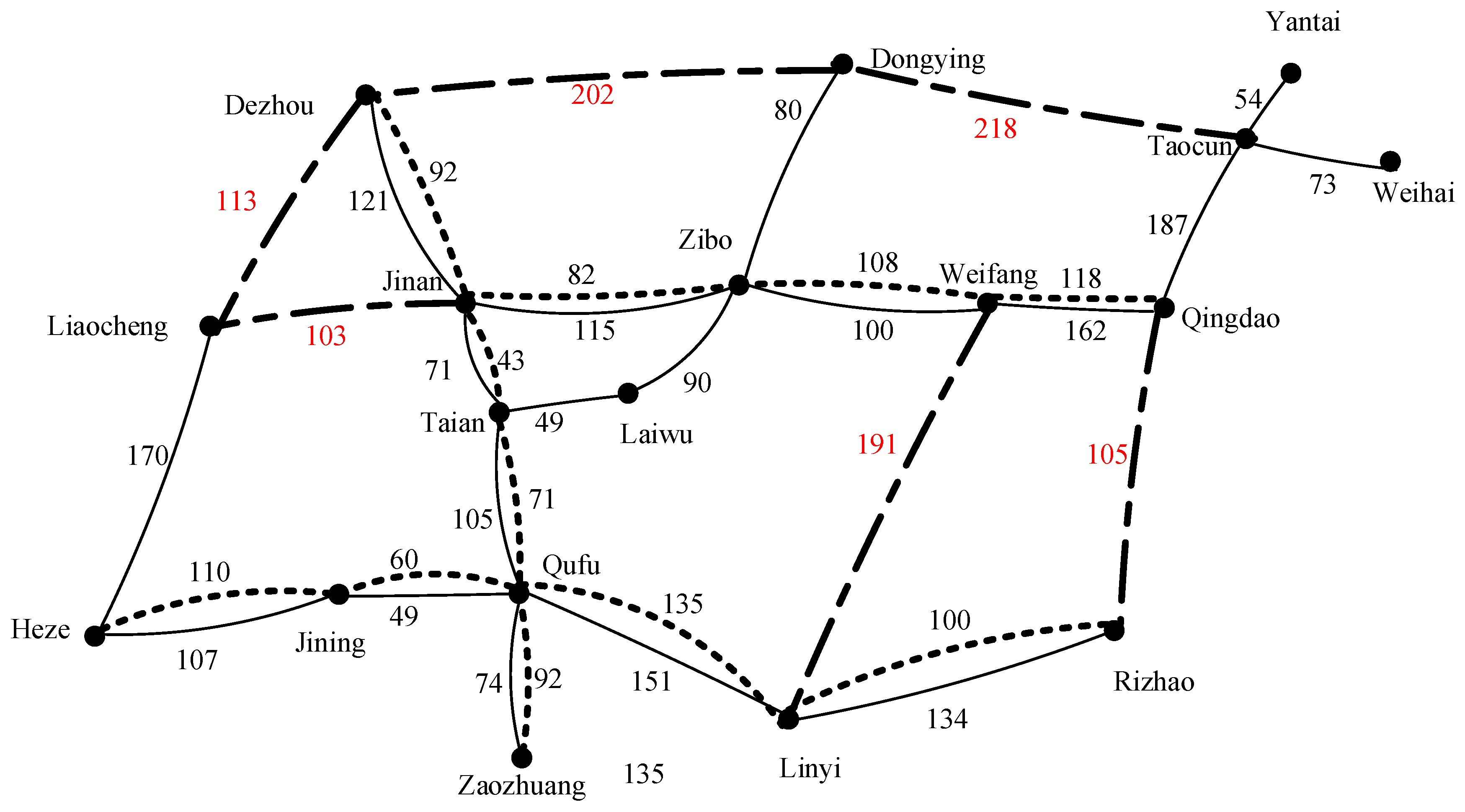
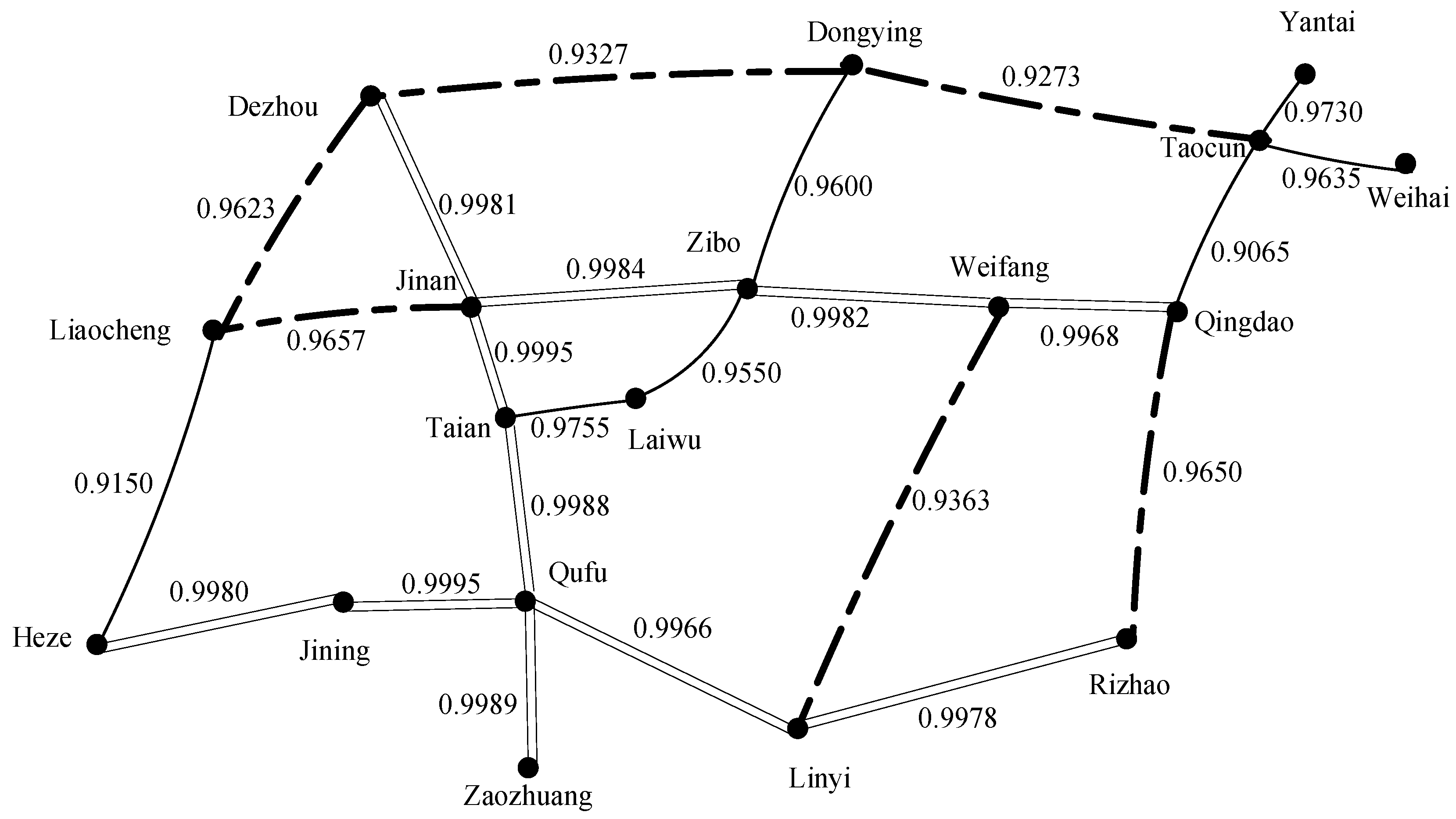
Firstly, we should determine the direct connection probability of between the neighboring nodes. As we can see that the longer a railway section is, the more likely it will go wrong. Therefore, we define $p_{i,j}^{NB}$ (direct connection probability of between the neighboring nodes) as $1-\frac{s_{ij}}{3000}$ when the railway is high-speed railway and as $1-\frac{s_{ij}}{2000}$ when the railway is normal-speed railway, because the high-speed railway is more reliable than the normal-speed railway. According to the estimation given by the railway managers, it is very likely that the direct connection is disturbed when the length of a railway line reaches to 3000, while the number is 2000 on the normal-speed railway. Therefore, we define $p_{i,j}^{NB}$ as follows.

$$p_{i,j}^{NB}=\{\begin{array}{l}1-\frac{s_{ij}}{3000},\mathrm{if}\mathrm{the}\mathrm{railway}\mathrm{is}\mathrm{high}\mathrm{speed}\mathrm{type}\\ 1-\frac{s_{ij}}{2000},\mathrm{if}\mathrm{the}\mathrm{railway}\mathrm{is}\mathrm{normal}\mathrm{speed}\mathrm{type}\end{array}$$

(7)

In Equation (7), $s_{ij}$ is the length between two neighbor nodes, Node i and Node j.

Then, we will calculate the comprehensive connection probability between each pair of nodes in the network.

The requirements of the passengers should be satisfied and we can get the requirement OD will be loaded on the railway network. In emergencies, passenger transportation reliability is much more important than the transportation efficiency. Therefore, it is essential for us to optimize the railway topology, considering the OD requirement, especially in emergencies, to assure that we can transport the passengers continuously to reduce the losses. Therefore, we construct a mathematical model of optimizing the reliability of the railway topology to describe the problem and design the optimizing algorithm in this paper.

However, we have the dilemma that the investment in the construction of the railway network is limited. Therefore, we must fully use the investment to bring optimal improvement for the existing railway network. In the optimization model, we can take the investment as a constraint, turning it into a longest construction mileage restriction. The model of reliability optimization of railway network is described as

$$\max p_{}^{NET}$$

(8)

$${\displaystyle \sum _i{\displaystyle \sum _j{x}_{ij}^{\mathrm{OD}}\cdot s_{ij}^{\mathrm{OD}}\le s_{invest}}}$$

(9)

Equation (8) is the optimization goal of the model, which is the reliability.

Equation (9) is the restriction of the longest construction mileage of high-speed railway under the current investment.

4. Computing Case

In this paper, we took the railway network optimization problem of Shandong Province, China, as the computing case. The existing railway network of this province is shown in Figure 5. In the network, the black dot indicates the passenger transport hub, which can be a normal speed railway station or a high-speed railway station, or a passenger transport hub composed of both of them. We call them station nodes in this paper. The numbers near the solid lines are the lengths of the normal speed railway sections and the numbers near the dotted lines are the lengths of the high-speed railway sections.

A solid line refers to the existing ordinary speed railway line and a dotted line refers to the existing high-speed railway line. The problem is how to choose the pairs of cities to add high-speed railway under the condition of limited construction investment in order to optimize the railway line network to maximize the reliability of the railway network to deal with the railway passenger transport task under emergency conditions. We turned the restriction of investment into the restriction of mileage of new high-speed railway.

Table 4. The abbreviation of the station nodes.

City	Abbreviation
Liaocheng	LC
Heze	HZ
Jining	JNI
Dezhou	DZ
Jinan	JNA
Taian	TA
Qufu	QF
Zaozhuang	ZZ
Laiwu	LW
Linyi	LY
Dongying	DY
Zibo	ZB
Rizhao	RZ
Weifang	WF
Qingdao	QD
Taocun	TC
Yantai	YT
Weihai	WH

shows the abbreviation of the station nodes names in the railway network in this case. We took it for granted that the station nodes were the railway junctions, not only connecting the normal-speed railway sections, but also the high-speed railway sections. The mileage of high-speed railway should be built between the station nodes if we choose the two nodes as the end station nodes is listed in

Table 5. The length of the high-speed railway to be built.

	LC	HZ	JNI	DZ	JNA	TA	QF	ZZ	LW	LY	DY	ZB	RZ	WF	QD	TC	YT	WH
LC		145	128	113	103	103	133	219	153	260	261	189	335	284	393	464	490	557
HZ			-	255	215	178	141	172	226	259	375	287	364	366	450	553	588	644
JNI				227	146	98	-	92	132	162	292	203	264	272	348	454	490	545
DZ					-	-	-	-	179	313	202	165	361	259	389	422	447	507
JNA						-	-	-	67	203	161	83	255	180	298	361	392	452
TA							-	-	57	166	196	108	235	192	296	376	412	469
QF								-	94	-	252	164	227	227	308	413	446	501
ZZ									160	100	315	232	211	267	310	433	473	524
LW										135	160	72	186	139	239	323	360	417
LY											260	191	-	191	211	339	380	430
DY												88	236	91	214	218	243	302
ZB													203	99	224	275	308	367
RZ														147	105	244	285	328
WF															130	183	218	276
QD																142	181	221
TC																	39	94
YT																		57
WH

. We can see that the stations on the first column are the beginning stations of the railway section to be built and the stations on the first row are the end stations of the railway sections. That means they are the minimum length of the high-speed railway that should be built once we choose to build the railway between the two station nodes. We take it for granted that the longest high-speed railway that can be added to the railway network is 1000 km according to the investment. It is to say $s_{invest}=1000$ in this computing case.

We can see that in the real railway network, there are many rings, which make the calculation too complicated in this computing case. Additionally, it is not necessary to calculate the connection probability on the path that is too long for it, as it is not available for the trains to finish the trip on it, although it is available theoretically. However, in which situation do we believe that the path is too long? In railway passenger transportation work, the on-schedule rate is a most important indicator to evaluate the service quality. If we change the train path and make the train run on an alternate path, which may cause a serious delay, it is required to cancel the train according to the dispatching rules. However, it is hard to determine how many times the length of the alternate path is that of the original path when we must cancel the train. Generally, it is acceptable and recommended that the number is two in the daily dispatching work in China. Therefore, we assume that when a path is longer than twice of the shortest path, it is unavailable for the train in this paper.

Then we carried out the optimizing process according to the model presented in Section 3.3. We can see that there are many choices when building the new railway lines in the network. Nevertheless, we cannot build the high-speed railway lines as needed as we do, because the investment is unlimited. We should choose the plan that meets the constraints in the model and improves the reliability as possible as we can.

The first step was to calculate the direct connecting probability of each neighbored pair of station nodes. There are two kinds of connections in the network. One is that there is only one railway line connecting the two neighbored station nodes. The other is that there are two kinds of railway lines: normal-speed railway and high-speed railway between the two neighbored station nodes. The direct connection probability of the two kinds of connections can be calculated out according to the method presented in Section 3.1.

Firstly, we calculated the original connection reliability between each pair of station nodes before optimization. The computing results were shown in

Table 6. Reliability of each pair of the original railway network.

	LC	HZ	JNI	DZ	JNA	TA	QF	ZZ	LW	LY	DY	ZB	RZ	WF	QD	TC	YT	WH
LC		0.9150	0.9132	0.9089	0.9111	0.9116	0.9127	0.9117	0.8893	0.9096	0.8746	0.9110	0.9076	0.9094	0.9064	0.8217	0.7995	0.7917
HZ			0.9980	0.9173	0.9958	0.9963	0.9975	0.9964	0.9719	0.9941	0.9738	0.9957	0.9919	0.9939	0.9907	0.8981	0.8738	0.8654
JNI				0.9954	0.9978	0.9983	0.9995	0.9984	0.9738	0.9961	0.9578	0.9977	0.9939	0.9959	0.9927	0.8999	0.8756	0.8671
DZ					0.9981	0.9976	0.9959	0.9948	0.9969	0.993	0.9581	0.9980	0.9903	0.9947	0.9930	0.9002	0.8759	0.8673
JNA						0.9995	0.9983	0.9972	0.9988	0.9949	0.9599	0.9999	0.9927	0.9981	0.9949	0.9019	0.8775	0.8690
TA							0.9988	0.9977	0.9755	0.9954	0.9599	0.9999	0.9932	0.9981	0.9949	0.9019	0.8775	0.8690
QF								0.9989	0.9743	0.9966	0.9589	0.9987	0.9944	0.9969	0.9937	0.9008	0.8765	0.8679
ZZ									0.9732	0.9955	0.9578	0.9976	0.9933	0.9958	0.9926	0.8998	0.8755	0.8669
LW										0.9710	0.9168	0.9550	0.9689	0.9532	0.9502	0.8614	0.8381	0.8299
LY											0.9556	0.9953	0.9987	0.9935	0.9903	0.8977	0.8735	0.8650
DY												0.9600	0.9534	0.9583	0.9552	0.8659	0.8425	0.8343
ZB													0.9931	0.9982	0.9950	0.9020	0.8776	0.8691
RZ														0.9913	0.9881	0.8957	0.8716	0.8631
WF															0.9968	0.9036	0.8792	0.8706
QD																0.9065	0.8820	0.8734
TC																	0.9730	0.9635
YT																		0.9375
WH

. Then, we optimized the railway network of Shandong Province according to the optimization method presented in this paper. There are 153 0–1 variables in this case when we initialized the reliability optimization model. They were all set to be 0 when the optimization process started. It was matches with the original railway network to be optimized. The variables were $x_{i,j}$, i = 1, 2, 3, 4, 5, 6, 7, 8, 9, 10, 11, 12, 13, 14, 15, 16, 17, 18, j = i, i + 1, i + 2,…, and 17. They were listed as below.

$$\begin{array}{l}{x}_{1,2},x_{1,3},x_{1,4},x_{1,5},x_{1,6},x_{1,7},x_{1,8},x_{1,9},x_{1,10},x_{1,11},x_{1,12},x_{1,13},x_{1,14},x_{1,15},x_{1,16},x_{1,17},x_{1,18},\\ x_{2,3},x_{2,4},x_{2,5},x_{2,6},x_{2,7},x_{2,8},x_{2,9},x_{2,10},x_{2,11},x_{2,12},x_{2,13},x_{2,14},x_{2,15},x_{2,16},x_{2,17},x_{2,18},\\ x_{3,4},x_{3,5},x_{3,6},x_{3,7},x_{3,8},x_{3,9},x_{3,10},x_{3,11},x_{3,12},x_{3,13},x_{3,14},x_{3,15},x_{3,16},x_{3,17},x_{3,18},\\ x_{4,5},x_{4,6},x_{4,7},x_{4,8},x_{4,9},x_{4,10},x_{4,11},x_{4,12},x_{4,13},x_{4,14},x_{4,15},x_{4,16},x_{4,17},x_{4,18},\\ x_{5,6},x_{5,7},x_{5,8},x_{5,9},x_{5,10},x_{5,11},x_{5,12},x_{5,13},x_{5,14},x_{5,15},x_{5,16},x_{5,17},x_{5,18},\\ x_{6,7},x_{6,8},x_{6,9},x_{6,10},x_{6,11},x_{6,12},x_{6,13},x_{6,14},x_{6,15},x_{6,16},x_{6,17},x_{6,18},\\ x_{7,8},x_{7,9},x_{7,10},x_{7,11},x_{7,12},x_{7,13},x_{7,14},x_{7,15},x_{7,16},x_{7,17},x_{7,18},\\ x_{8,9},x_{8,10},x_{8,11},x_{8,12},x_{8,13},x_{8,14},x_{8,15},x_{8,16},x_{8,17},x_{8,18},\\ x_{9,10},x_{9,11},x_{9,12},x_{9,13},x_{9,14},x_{9,15},x_{9,16},x_{9,17},x_{9,18},\\ x_{10,11},x_{10,12},x_{10,13},x_{10,14},x_{10,15},x_{10,16},x_{10,17},x_{10,18},\\ x_{11,12},x_{11,13},x_{11,14},x_{11,15},x_{11,16},x_{11,17},x_{11,18},\\ x_{12,13},x_{12,14},x_{12,15},x_{12,16},x_{12,17},x_{12,18},\\ x_{13,14},x_{13,15},x_{13,16},x_{13,17},x_{13,18},\\ x_{14,15},x_{14,16},x_{14,17},x_{14,18},\\ x_{15,16},x_{15,17},x_{15,18},\\ x_{16,17},x_{16,18},\\ x_{17,18}\end{array}$$

In the optimization process, the 0–1 variables were changed according to the computing rules, and the connection reliability of the station nodes and that of the whole network were calculated out in each iteration. The changing process is shown in Figure 6.

The optimization goal, the connection reliability of the station nodes, tended to be stable after 400 calculation iterations. The optimal solution in this case is that $x_{1,4}=x_{1,5}=x_{4,11}=x_{10,14}=x_{11,16}=x_{13,15}=1$.

Other decision variables were 0. Then, the connection reliability of all the station nodes in the network were presented in

Table 7. Connection reliability of all the station nodes in Shandong Province.

	Connection Reliability before Optimization	Connection Reliability after Optimization	Difference
LC	0.8885	0.9870	0.0985
HZ	0.9627	0.9803	0.0176
JNI	0.9677	0.9911	0.0234
DZ	0.9633	0.9867	0.0234
JNA	0.9697	0.9927	0.0230
TA	0.9685	0.9914	0.0229
QF	0.9683	0.9911	0.0228
ZZ	0.9672	0.9902	0.0230
LW	0.9411	0.9651	0.0240
LY	0.9656	0.9745	0.0089
DY	0.9319	0.9690	0.0371
ZB	0.9673	0.9886	0.0213
RZ	0.9636	0.9794	0.0158
WF	0.9663	0.9894	0.0231
QD	0.9645	0.9750	0.0105
TC	0.8996	0.9653	0.0657
YT	0.8769	0.9408	0.0639
WH	0.8689	0.9380	0.0691

and the connection reliability of each pair of the station nodes were calculated out and listed in

Table 8. Reliability of each pair of the optimized railway network according to the computing results.

	LC	HZ	JNI	DZ	JNA	TA	QF	ZZ	LW	LY	DY	ZB	RZ	WF	QD	TC	YT	WH
LC		0.9150	0.9997	0.9986	0.9986	0.9998	0.9997	0.9986	0.9974	0.9963	0.9957	0.9985	0.9941	0.994	0.9963	0.9865	0.9599	0.9506
HZ			0.9980	0.9137	0.9995	0.9996	0.9975	0.9964	0.9751	0.9941	0.9966	0.9994	0.9919	0.9963	0.9941	0.9866	0.9600	0.9506
JNI				0.9978	0.9997	0.9983	0.9995	0.9984	0.9738	0.9961	0.9968	0.9982	0.9939	0.9963	0.9986	0.9888	0.9621	0.9527
DZ					0.9981	0.9976	0.9964	0.9953	0.9969	0.9930	0.9971	0.9996	0.9908	0.9962	0.9986	0.9888	0.9621	0.9527
JNA						0.9995	0.9983	0.9972	0.9988	0.9949	0.9971	0.9999	0.9927	0.9981	0.9989	0.9891	0.9624	0.9530
TA							0.9988	0.9977	0.9755	0.9954	0.9966	0.9999	0.9932	0.9981	0.9989	0.9891	0.9624	0.9530
QF								0.9989	0.9743	0.9966	0.9954	0.9987	0.9944	0.9998	0.9966	0.9891	0.9624	0.9530
ZZ									0.9732	0.9955	0.9943	0.9988	0.9933	0.9987	0.9955	0.988	0.9613	0.9520
LW										0.9969	0.9168	0.9550	0.9947	0.9533	0.9502	0.9447	0.9192	0.9102
LY											0.9597	0.9997	0.9987	0.9974	0.9975	0.9042	0.8798	0.8712
DY												0.9600	0.9581	0.9932	0.9929	0.9273	0.9023	0.8935
ZB													0.9957	0.9982	0.999	0.9892	0.9625	0.9531
RZ														0.9975	0.9999	0.9064	0.8819	0.9733
WF															0.9968	0.9893	0.9626	0.9532
QD																0.9065	0.8820	0.8734
TC																	0.9730	0.9635
YT																		0.9375
WH

. The optimized railway network is shown in Figure 7 and Figure 8. The calculation details can be found in Appendix A.

5. Results Analysis

From Table 7, we can see that the connection reliability of all the station nodes increased, especially that of Liaocheng, Taocun, Yantai, and Weihai. It is because only a railway line is connected with Liaocheng, and it is located at the most northwest of Shandong Province. After the optimization, the high speed railway lines between Liaocheng and Dezhou and Liaocheng and Jinan are both added in the railway network. The connection between it and other stations are greatly enhanced. The same happened at Dongying. Taocun is at the fork of the railroad to Yantai and Weihai. The optimization plan required the addition of a new high-speed railway line between Taocun and Dongying, so the connection between Taocun and other station nodes is strengthened. As a result, the connection reliability of Yantai and Weihai is also improved.

As the capital of Shandong Province, Jinan has the connection reliability of 0.9927, which is the biggest among all of the cities after optimization. It assures the connection reliability from Jinan city to other cities of Shandong Province. It is in line with its position in the province. Taian and Qufu have the second largest connection reliability, for they are both already on Beijing–Shanghai high-speed railway, which travels between the two most important tourist cities in Shandong Province. The high-speed railway lines added between Liaocheng and Jinan and Liaocheng and Dezhou further strengthen the railway network, enlarging their connection reliability value. Another two cities whose connection reliability value are higher than 0.99 are Zaozhuang and Jining. The reason is that Zaozhuang is also on the Beijing–Shanghai high-speed railway, and Jining is already on South Shandong high-speed railway. We can see that the optimization is focused on east and north of the railway network, which is weak in the original network. It proves that the optimization rules are efficient.

Additionally, the connection reliability of the whole railway network is 0.9445 before the optimization, and it increases to 0.9775 after the optimization, which means that the connection reliability of the whole railway network is improved and the optimization method is correct and efficient.

The length that is added into the railway network was 932 km, which is shorter than the length that is limited by the investment. Although the investment is limited, we should try our best to use the investment fully to strengthen the railway transportation system.

We can see that high-speed railway is added between several pairs of station nodes due to the plan, such as Jinan and Liaocheng, Qingdao and Rizhao, and Weifang and Linyi. Between these cities, there was no railway before, and it is more necessary to build high-speed railway between them. The plan not only makes the cities connect each other efficiently, but also strengthens the whole railway network. It forms rings in the railway network, making the topology stronger, and improves the reliability of the whole network. It means that the whole network will keep connectivity when the emergencies disturb the railway system, blocking some of the railway sections. There is no doubt that the railway connection reliability is greatly optimized in this computing case.

6. Conclusions

In this paper, we have modeled a railway network reliability optimization problem based on the probability theory. The definitions of direct connection probability, connection reliability between nodes, connection reliability of a node, and network connection reliability presented in this paper brings new ideas when studying the reliability of the railway network. It describes influencing factors of the reliability, such as the length of the railway section and the emergency probability, and some innovative definitions on the railway network are proposed, such as neighboring stations’ direct connection probability, connection reliability between two station nodes on a path, connection reliability between two station nodes, station node connection reliability, and railway network connection reliability. It is an innovate approach to optimizing the railway network.

The reliability optimization model is based on the probability theory, considering the fact that the longer the operation railway mileage is, the more likely the railway operation work will be disturbed. Three computing cases are presented to illustrate the computing method for computing the reliability of the connection reliability between two station nodes, which is the key to calculating the reliability. The direct connection probability calculation method is based on the probability theory, using the concept of probability felicitously, and the definition of connection between two station nodes takes all the available paths between the two nodes. It not only meets the rules of mathematical theory, but also considers the real railway operation rules.

The model describes the railway network reliability optimization problem precisely, taking the railway construction investment as the constraint, which is turned into the railway line construction mileage constraint, establishing the connection between investment and railway network optimization. The computing case proved the rationality and availability of the railway network optimization model. The generated building plan of high-speed railway falls in with the real construction requirements.

Future study will continuously focus on the optimization approach of more complicated railway networks, generating and optimizing the approach to be fit for more complex railway network optimization problems.

References

1. Lee, T.S.; Ghosh, S. Stability of RYNSORD–A decentralized algorithm for railway networks under perturbations. IEEE Trans. Veh. Tech. 2001, 50, 287–301. [Google Scholar] [CrossRef]
2. Sen, P.; Dasgupta, S.; Chatterjee, A.; Sreeram, P.A.; Mukherjee, G.; Manna, S.S. Small-world properties of the Indian railway network. Phys. Rev. 2003, 67, 36106. [Google Scholar] [CrossRef] [PubMed] [Green Version]
3. Seaton, K.A.; Hackett, L.M. Stations, trains and small-world networks. Phys. Sect. A 2004, 339, 635–644. [Google Scholar] [CrossRef] [Green Version]
4. Chen, S.; Hsu, S.C.; Tseng, C.T.; Yan, K.H.; Chou, H.Y.; Too, T.M. Analysis of rail potential and stray current for Taipei Metro. IEEE Trans. Veh. Technol. 2006, 55, 67–75. [Google Scholar] [CrossRef]
5. Li, W.; Cai, X. Empirical analysis of a scale-free railway network in China. Phys. Sect. A Stat. Theor. Phys. 2007, 382, 693–703. [Google Scholar] [CrossRef]
6. Ghosh, S.; Banerjee, A.; Sharma, N.; Agarwal, S.; Ganguly, N. Statistical analysis of the Indian railway network: A complex network approach. Acta Phys. Pol. B Proc. Suppl. 2011, 2, 123–138. [Google Scholar] [CrossRef]
7. Martí-Henneberg, J. European integration and national models for railway networks (1840–2010). J. Transp. Geogr. 2013, 26, 126–138. [Google Scholar] [CrossRef]
8. Innocenti, A.; Marini, L.; Meli, E.; Pallini, G.; Rindi, A. Development of a wear model for the analysis of complex railway networks. Wear 2014, 309, 174–191. [Google Scholar] [CrossRef] [Green Version]
9. Meng, X.; Xiang, W.; Wang, L. Controllability of train service network. Math. Probl. Eng. 2015, 631492. [Google Scholar] [CrossRef] [Green Version]
10. Yang, Y.H.; Liu, Y.X.; Zhou, M.X.; Li, F.X.; Sun, C. Robustness assessment of urban rail transit based on complex network theory: A case study of the Beijing Subway. Saf. Sci. 2015, 79, 149–162. [Google Scholar] [CrossRef]
11. Hu, M.; Zhong, Z.; Ni, M.; He, R. Analysis of link lifetime with auto-correlated shadowing in high-speed railway networks. IEEE Commun. Lett. 2015, 19, 2106–2109. [Google Scholar] [CrossRef]
12. Wandelt, S.; Wang, Z.; Sun, X. Worldwide railway skeleton network: Extraction methodology and preliminary analysis. IEEE Trans. Intell. Transp. Syst. 2017, 18, 2206–2216. [Google Scholar] [CrossRef]
13. Zhao, W.; Martin, U.; Cui, Y. Operational risk analysis of block sections in the railway network. J. Rail Transp. Plan. Manag. 2017, 7, 245–262. [Google Scholar] [CrossRef]
14. Lu, Q. Modeling network resilience of rail transit under operational incidents. Transp. Res. Part A 2018, 117, 227–237. [Google Scholar] [CrossRef]
15. Caset, F.; Vale, D.S.; Viana, C.M. Urban Networks Special Issue: Measuring the accessibility of railway stations in the brussels regional express network: A node-place modeling approach. Netw. Spat. Econ. 2018, 18, 1–36. [Google Scholar]
16. Alessio, P.; Guillem, M.; Aseel, A.; Samuel, J.; Stephen, J.; Alan, W.; Weisi, G.; Liz, V. Resilience or robustness: Identifying topological vulnerabilities in rail networks. R. Soc. Open Sci. 2019, 2, 181301. [Google Scholar]
17. Cats, O.; Krishnakumari, P. Metropolitan rail network robustness. Phys. A Stat. Mech. Appl. 2020, 549, 124317. [Google Scholar] [CrossRef]
18. Olentsevich, V.A.; Belogolov, Y.I.; Grigoryeva, N.N. Analysis of reliability and sustainability of organizational and technical systems of railway transportation process. IOP Conf. Ser. Mater. Sci. Eng. 2020, 832, 012061. [Google Scholar] [CrossRef]
19. Fang, C.; Dong, P.; Fang, Y.; Zio, E. Vulnerability analysis of critical infrastructure under disruptions: An application to China Railway High-speed. Proc. Inst. Mech. Eng. Part O J. Risk Reliab. 2020, 234, 235–245. [Google Scholar] [CrossRef]
20. Zhu, H.; Zhang, C. Expanding a complex networked system for enhancing its reliability evaluated by a new efficient approach. Reliab. Eng. Syst. Saf. 2019, 188, 205–220. [Google Scholar] [CrossRef]
21. Gu, S. Reliability analysis of high-speed railway network. Proc. Inst. Mech. Eng. Part O J. Risk Reliab. 2019, 233, 1060–1073. [Google Scholar] [CrossRef]
22. Hossain, M.M.; Alam, S. A complex network approach towards modeling and analysis of the Australian Airport Network. J. Air Transp. Manag. 2017, 60, 1–9. [Google Scholar] [CrossRef]
23. Daganzo, C.F. Structure of competitive transit networks. Transp. Res. Part B Methodol. 2010, 44, 434–446. [Google Scholar] [CrossRef] [Green Version]
24. Sullivan, J.L.; Aultman-Hall, L.; Novak, D.C. A review of current practice in network disruption analysis and an assessment of the ability to account for isolating links in transportation networks. Transp. Lett. 2009, 1, 271–280. [Google Scholar] [CrossRef]
25. Tian, Z.W.; Zhang, Z.; Wang, H.F.; Ma, L. Complexity analysis on public transport networks of 97 large- and medium-sized cities in China. Int. J. Mod. Phys. B 2018, 32. [Google Scholar] [CrossRef]
26. Currie, G.; Delbosc, A. Assessing bus rapid transit system performance in Australasia. Res. Transp. Econ. 2014, 48, 142–151. [Google Scholar] [CrossRef]
27. Reynaud, F.; Sider, T.; Hatzopoulou, M.; Eluru, N. Extending the network robustness index to include emissions: A holistic framework for link criticality analysis for Montreal transportation system. Transp. Lett. 2016, 10, 302–315. [Google Scholar] [CrossRef]
28. Doana, K.; Ukkusuria, S. Measuring inefficiency in dynamic traffic networks: A numerical study. Transp. Lett. 2015, 7, 154–167. [Google Scholar] [CrossRef]
29. Loustau, P.; Morency, C.; Trépanier, M.; Gourvil, L. Travel time reliability on a highway network: Estimations using floating car data. Transp. Lett. 2010, 2, 27–37. [Google Scholar] [CrossRef]
30. Sun, D.; Guan, S. Measuring vulnerability of urban metro network from line operation perspective. Transp. Res. Part A 2016, 94, 348–359. [Google Scholar] [CrossRef]
31. Zhang, J.H.; Xu, X.M.; Hong, L.; Wang, S.; Fei, Q. Networked analysis of the Shanghai subway network, in China. Phys. A 2011, 390, 4562–4570. [Google Scholar] [CrossRef]
32. Febbraro, A.D.; Giglio, D.; Sacco, N. On analyzing the vulnerabilities of a railway network with Petri nets. Transp. Res. Procedia 2017, 27, 553–560. [Google Scholar] [CrossRef]
33. Li, M.; Wang, Y.; Jia, L.; Cui, Y. Risk propagation analysis of urban rail transit based on network model. Alex. Eng. J. 2020, 59, 1319–1331. [Google Scholar] [CrossRef]
34. Jiang, R.Y.; Lu, Q.C.; Peng, Z.R. A station-based rail transit network vulnerability measure considering landuse dependency. J. Transp. Geogr. 2018, 66, 10–18. [Google Scholar] [CrossRef]
35. Zhong, H.L.; Wang, J.; Yip, T.L.; Gu, Y. An innovative gravity-based approach to assess vulnerability of a Hazmat road transportation network: A case study of Guangzhou, China. Transp. Res. Part D 2018, 62, 659–671. [Google Scholar] [CrossRef]
36. Ouyang, M.; Zhao, L.J.; Hong, L.; Pan, Z.Z. Comparisons of complex network based models and real train flowmodel to analyze Chinese railway vulnerability. Reliab. Eng. Sys. Saf. 2014, 123, 38–46. [Google Scholar] [CrossRef]
37. Xiao, X.M.; Jia, L.M.; Wang, Y.H. Correlation between heterogeneity and vulnerability of subway networks based on passenger flow. J. Rail Transp. Plan. Manag. 2018, 8, 145–157. [Google Scholar] [CrossRef]
38. Oliveira, E.L.D.; Portugal, L.D.S.; Junior, W.P. Indicators of reliability and vulnerability: Similarities anddifferences in ranking links of a complex road system. Transp. Res. Part A 2016, 88, 195–208. [Google Scholar] [CrossRef]
39. Núñez, E.R.; Palomares, J.C.G. Measuring the vulnerability of public transport networks. J. Transp. Geogr. 2014, 35, 50–63. [Google Scholar] [CrossRef] [Green Version]
40. Balijepalli, C.; Oppong, O. Measuring vulnerability of road network considering the extent of serviceability of critical road links in urban areas. J. Transp. Geogr. 2014, 39, 145–155. [Google Scholar] [CrossRef]
41. Taylor, M.A.P.; Susilawati. Remoteness and accessibility in the vulnerability analysis of regional road networks. Transp. Res. Part A 2012, 46, 761–771. [Google Scholar] [CrossRef]
42. Jenelius, E.; Mattsson, L.G. Road network vulnerability analysis of area-covering disruptions: A grid-based approach with case study. Transp. Res. Part A 2012, 46, 746–760. [Google Scholar] [CrossRef]
Figure 1. Network in Case 1.
Sustainability 12 09805 g001
Figure 2. Network in Case 2.
Sustainability 12 09805 g002
Figure 3. Network in Case 3.
Sustainability 12 09805 g003
Figure 4. A simple sketch map of the path between node i to node j.
Sustainability 12 09805 g004
Figure 5. Existing railway network of Shandong Province with section length.
Sustainability 12 09805 g005
Figure 6. Changing process of connection reliability of the station nodes and the whole network in the optimization. Note: The value under abscissa stands for the times of calculation iteration. Note: (a) is the changing process of connection reliability of Liaocheng Station. (b) is the changing process of connection reliability of Heze Station. (c) is the changing process of connection reliability of Jinan Station. (d) is the changing process of connection reliability of Linyi Station. (e) is the changing process of connection reliability of Dongying Station. (f) is the changing process of connection reliability of Rizhao Station. (g) is the changing process of connection reliability of Weifang Station. (h) is the changing process of connection reliability of Qingdao Station. (i) is the changing process of connection reliability of Taocun Station. (j) is the changing process of connection reliability of the whole network.
Sustainability 12 09805 g006
Figure 7. Optimal plan of railway network of Shandong Province in this paper. Note: The red numbers are the lengths of the high-speed railway lines between the stations.
Sustainability 12 09805 g007
Figure 8. Optimal plan of railway network of Shandong Province with direct connection probability.
Sustainability 12 09805 g008