Comparative Assessment of Carbon Footprints of Selected Organizations: The Application of the Enhanced Bilan Carbone Model


Abstract
1. Introduction
2. Materials and Methods
2.1. The Method Used for Calculating CF
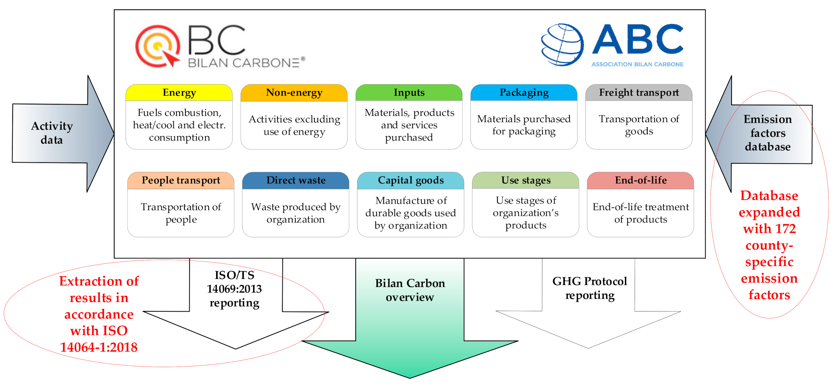
2.2. Enhanced Bilan Carbone® model
2.3. Uncertainty Estimation
2.4. CF Calculation Process
3. Results and Discussion
3.1. Results of CF Calculation
3.2. Uncertainty of the CF calculations
3.3. Key Sources Analysis
3.4. Comparison of the CF Results
3.5. CF Reduction
4. Conclusions
Supplementary Materials
Author Contributions
Funding
Acknowledgments
Conflicts of Interest
References
- World Meteorological Organization. WMO Statement on the Status of the Global Climate in 2019, WMO-No. 1248. Strategic Communications Office: Geneva, Switzerland, 2020. Available online: https://library.wmo.int/doc_num.php?explnum_id=10211 (accessed on 15 October 2020).
- Intergovernmental Panel on Climate Change. Climate Change 2013—The Physical Science Basis. Working Group I Contribution to the Fifth Assessment Report of the Intergovernmental Panel on Climate Change, WMO, UNEP. New York, USA. 2013. Available online: https://www.ipcc.ch/site/assets/uploads/2018/02/WG1AR5_all_final.pdf (accessed on 15 October 2020).
- Scrutton, A.; Jones, N.; Akana, D.; Capon, A.; Gaffney, O.; Jacob, D.; Luers, A.; Rockström, J.; Scholes, R.; Whiteman, G. Our Future on Earth, Science Insights into our Planet and Society. Future Earth—Research, Innovation, Sustainability. 2020. Available online: https://futureearth.org/publications/our-future-on-earth/ (accessed on 17 November 2020).
- Azapagic, A.; Perdan, S. Sustainable Development in Practice, Case Studies for Engineers and Scientists; Chapter 1: The Concept of Sustainable Development and its Practical Implications; Wiley-Blackwell: Chichester, UK, 2011. [Google Scholar]
- International Union for Conservation of Nature. World Conservation Strategy; UNEP; WWF; FAO; UNESCO: Gland, Switzerland, 1980; Available online: http://www.a21italy.it/medias/31C2D26FD81B0D40.pdf (accessed on 15 October 2020).
- World Commission on Environment and Development. Report of the World Commission on Environment and Development: Our Common Future; Oxford University Press: Oslo, Norway, 1987. Available online: https://sustainabledevelopment.un.org/content/documents/5987our-common-future.pdf (accessed on 15 October 2020).
- Faria, P.; van der Vlugt, I.; Griffn, P.; Heede, P. The Carbon Majors Database, CDP Carbon Majors Report 2017, 100 Fossil Fuel Producers and Nearly 1 Trillion Tonnes of Greenhouse Gas Emissions; CDP Driving Sustainable Economies: London, UK, 2017. [Google Scholar]
- Zvezdov, D.; Hack, S. Carbon footprinting of large product portfolios. Extending the use of Enterprise Resource Planning systems to carbon information management. J. Clean. Prod. 2016, 135, 1267–1275. [Google Scholar] [CrossRef]
- Pandey, D.; Agrawal, M.; Pandey, J.S. Carbon Footprint: Current Methods of Estimation. Environ. Monit. Assess. 2011, 178, 35–160. [Google Scholar] [CrossRef]
- Dawkins, C.; Fraas, J.W. Coming Clean: The Impact of Environmental Performance and Visibility on Corporate Climate Change Disclosure. J. Bus. Ethics 2011, 100, 303–322. [Google Scholar] [CrossRef]
- Minx, J.C.; Wiedmann, T.; Wood, R.; Peters, G.P.; Lenzen, M.; Owen, A.; Scott, K.; Barrett, J.; Hubacek, K.; Baiocchi, G.; et al. Input–Output Analysis and Carbon Footprinting: An Overview of Applications. Econ. Syst. Res. 2009, 21, 187–216. [Google Scholar] [CrossRef]
- Berners-Lee, M.; Howard, D.C.; Moss, J.; Kaivanto, K.; Scott, W.A. Greenhouse gas footprinting for small businesses—The use of input–output data. Sci. Total Environ. 2011, 409, 883–891. [Google Scholar] [CrossRef]
- Navarro, A.; Puig, R.; Fullana-i-Palmer, P. Product vs corporate carbon footprint: Some methodological issues. A case study and review on the wine sector. Sci. Total Environ. 2017, 581–582, 722–733. [Google Scholar] [CrossRef]
- Chen, J.X.; Chen, J. Supply chain carbon footprinting and responsibility allocation under emission regulations. J. Environ. Manag. 2017, 188, 255–267. [Google Scholar] [CrossRef]
- Lombardi, M.; Laiola, E.; Tricase, C.; Rana, R. Assessing the urban carbon footprint: An overview. Environ. Impact Assess. Rev. 2017, 66, 43–52. [Google Scholar] [CrossRef]
- GHG Protocol. Global Protocol for Community-Scale Greenhouse Gas Emission Inventories. An Accounting and Reporting Standard for Cities. World Resources Institute, C40 Cities Climate Leadership Group and ICLEI—Local Governments for Sustainability, 2014 (ISBN 1-56973-846-7). USA. 2014. Available online: https://ghgprotocol.org/sites/default/files/standards/GHGP_GPC_0.pdf (accessed on 12 November 2020).
- Covenant of Mayors & Mayors Adapt Offices; Joint Research Centre of the European Commission. The Covenant of Mayors for Climate and Energy Reporting Guidelines. Version 1.0. 2016. Available online: https://www.covenantofmayors.eu/IMG/pdf/Covenant_ReportingGuidelines.pdf (accessed on 12 November 2020).
- Roibas, L.; Loiseau, E.; Hospido, A. Determination of the carbon footprint of all Galician production and consumption activities: Lessons learnt and guidelines for policymakers. J. Environ. Manag. 2017, 198, 289–299. [Google Scholar] [CrossRef]
- Padgett, J.P.; Steinemann, A.C.; Clarke, J.H.; Vandenbergh, M.P. A comparison of carbon calculators. Environ. Impact Assess. Rev. 2008, 28, 106–115. [Google Scholar] [CrossRef]
- Kenny, T.; Gray, N.F. Comparative performance of six carbon footprint models for use in Ireland. Environ. Impact Assess. Rev. 2009, 29, 1–6. [Google Scholar] [CrossRef]
- Birnik, A. An evidence-based assessment of online carbon calculators. Int. J. Greenh. Gas Control 2013, 17, 280–293. [Google Scholar] [CrossRef]
- Mulrow, J.; Machaj, K.; Deanes, J.; Derrible, S. The state of carbon footprint calculators: An evaluation of calculator design and user interaction features. Sustain. Prod. Consum. 2019, 18, 33–40. [Google Scholar] [CrossRef]
- Harangozo, G.; Szigeti, C. Corporate carbon footprint analysis in practice–with a special focus on validity and reliability issues. J. Clean. Prod. 2017, 167, 1177–1183. [Google Scholar] [CrossRef]
- ISO 14064-1. Greenhouse gases—Part 1: Specification with Guidance at the Organization Level for Quantification and Reporting of Greenhouse Gas Emissions and Removals (ISO 14064-1:2006); International Organization for Standardization: Geneva, Switzerland, 2006. [Google Scholar]
- GHG Protocol Corporate. A Corporate Accounting and Reporting Standard (Revised Edition). World Resources Institute and World Business Council for Sustainable Development, 2004 (ISBN 1-56973-568-9). USA. 2004. Available online: https://ghgprotocol.org/sites/default/files/standards/ghg-protocol-revised.pdf (accessed on 15 October 2020).
- GHG Protocol Corporate. Corporate Value Chain (Scope 3) Accounting and Reporting Standard. World Resources Institute and World Business Council for Sustainable Development, 2011 (ISBN 978-1-56973-772-9). USA. 2011. Available online: https://ghgprotocol.org/sites/default/files/standards/Corporate-Value-Chain-Accounting-Reporing-Standard_041613_2.pdf (accessed on 15 October 2020).
- ISO 14064-1. Greenhouse Gases—Part 1: Specification with Guidance at the Organization Level for Quantification and Reporting of Greenhouse Gas Emissions and Removals (ISO 14064-1:2018); International Organization for Standardization: Geneva, Switzerland, 2018. [Google Scholar]
- Radonjič, G.; Tompa, S. Carbon footprint calculation in telecommunications companies—The importance and relevance of scope 3 greenhouse gases emissions. Renew. Sustain. Energy Rev. 2018, 98, 361–375. [Google Scholar] [CrossRef]
- Larsen, H.N.; Pettersen, J.; Solli, C.; Hertwich, E.G. Investigating the Carbon Footprint of a University—The case of NTNU. J. Clean. Prod. 2013, 48, 39–47. [Google Scholar] [CrossRef]
- Vasquez, L.; Iriarte, A.; Almeida, M.; Villalobos, P. Evaluation of greenhouse gas emissions and proposals for their reduction at a university campus in Chile. J. Clean. Prod. 2015, 108, 924–930. [Google Scholar] [CrossRef]
- Ridhosari, R.; Rahman, A. Carbon footprint assessment at Universitas Pertamina from the scope of electricity, transportation, and waste generation: Toward a green campus and promotion of environmental sustainability. J. Clean. Prod. 2019, 246, 119172. [Google Scholar] [CrossRef]
- Yañez, P.; Sinha, A.; Vásquez, M. Carbon Footprint Estimation in a University Campus: Evaluation and Insights. Sustainability 2020, 12, 181. [Google Scholar] [CrossRef]
- Robinson, A.J.; Tewkesbury, A.; Kemp, S.; Williams, I.D. Towards a Universal Carbon Footprint Standard: A Case Study of Carbon Management at Universities. J. Clean. Prod. 2018, 172, 4435–4455. [Google Scholar] [CrossRef]
- LIFE Clim’Foot Project. Climate Governance: Implementing Public Policies to Calculate and Reduce Organizations Carbon Footprint. LIFE14 GIC/FR/000475. 2018. Available online: http://www.climfoot-project.eu/ (accessed on 15 October 2020).
- Jurić, Ž.; Ljubas, D.; Đurđević, D.; Luttenberger, L. Implementation of the Harmonised Model for Carbon Footprint Calculation on Example of the Energy Institute in Croatia. J. Sustain. Dev. Energy Water Environ. Syst. 2019, 7, 368–384. [Google Scholar] [CrossRef]
- ISO/TR 14069. Greenhouse Gases—Quantification and Reporting of GHG Emissions for Organizations—Guidance for the Application of ISO 14064-1 (ISO/TR 14069:2013); International Organization for Standardization: Geneva, Switzerland, 2013. [Google Scholar]
- ADEME. Methodology Guide—Version 6.1—Objectives and Accounting Principles. Bilan Carbone—Companies, Local Authorities, Regions. The French Environment and Energy Management Agency, France. 2010. Available online: https://docplayer.net/3317100-Bilan-carbone-companies-local-authorities-regions-methodology-guide-version-6-1-objectives-and-accounting-principles.html (accessed on 15 October 2020).
- LIFE Clim’Foot Project. National Database of Emission Factors, Croatia. LIFE14 GIC/FR/000475. EIHP and EKONERG. 2017. Available online: http://www.climfoot-project.eu/en/practical-case-croatia (accessed on 15 October 2020).
- Intergovernmental Panel on Climate Change. IPCC Good Practice Guidance and Uncertainty Management in National Greenhouse Gas Inventories. WMO; UNEP: Kanagawa, Japan, 2001; Available online: https://www.ipcc-nggip.iges.or.jp/public/gp/english/ (accessed on 15 October 2020).
- Alvarez, S.; Blanquer, M.; Rubio, A. Carbon footprint using the compound method based on financial accounts. The case of the School of Forestry Engineering, Technical University of Madrid. J. Clean. Prod. 2014, 66, 224–232. [Google Scholar] [CrossRef]
- Mendoza-Flores, R.; Quintero-Ramırez, R.; Ortiz, I. The carbon footprint of a public university campus in Mexico City. Carbon Manag. 2019, 10, 501–511. [Google Scholar] [CrossRef]
- Güereca, L.P.; Torres, T.; Noyola, A. Carbon Footprint as a basis for a cleaner research institute in Mexico. J. Clean. Prod. 2013, 47, 396–403. [Google Scholar] [CrossRef]


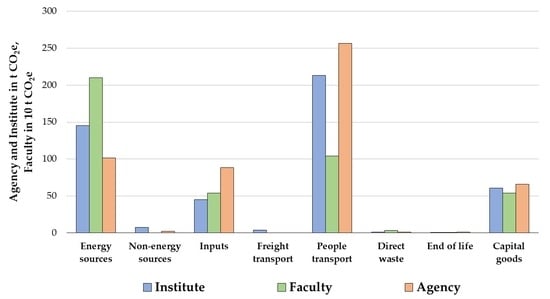
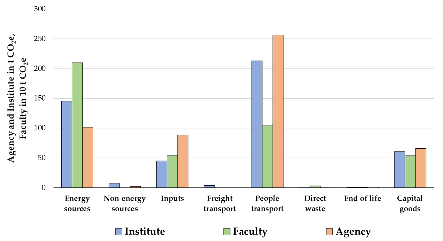
| BC Emission Categories | Agency | Faculty | Institute | |||
|---|---|---|---|---|---|---|
| t CO2 e | % | t CO2 e | % | t CO2 e | % | |
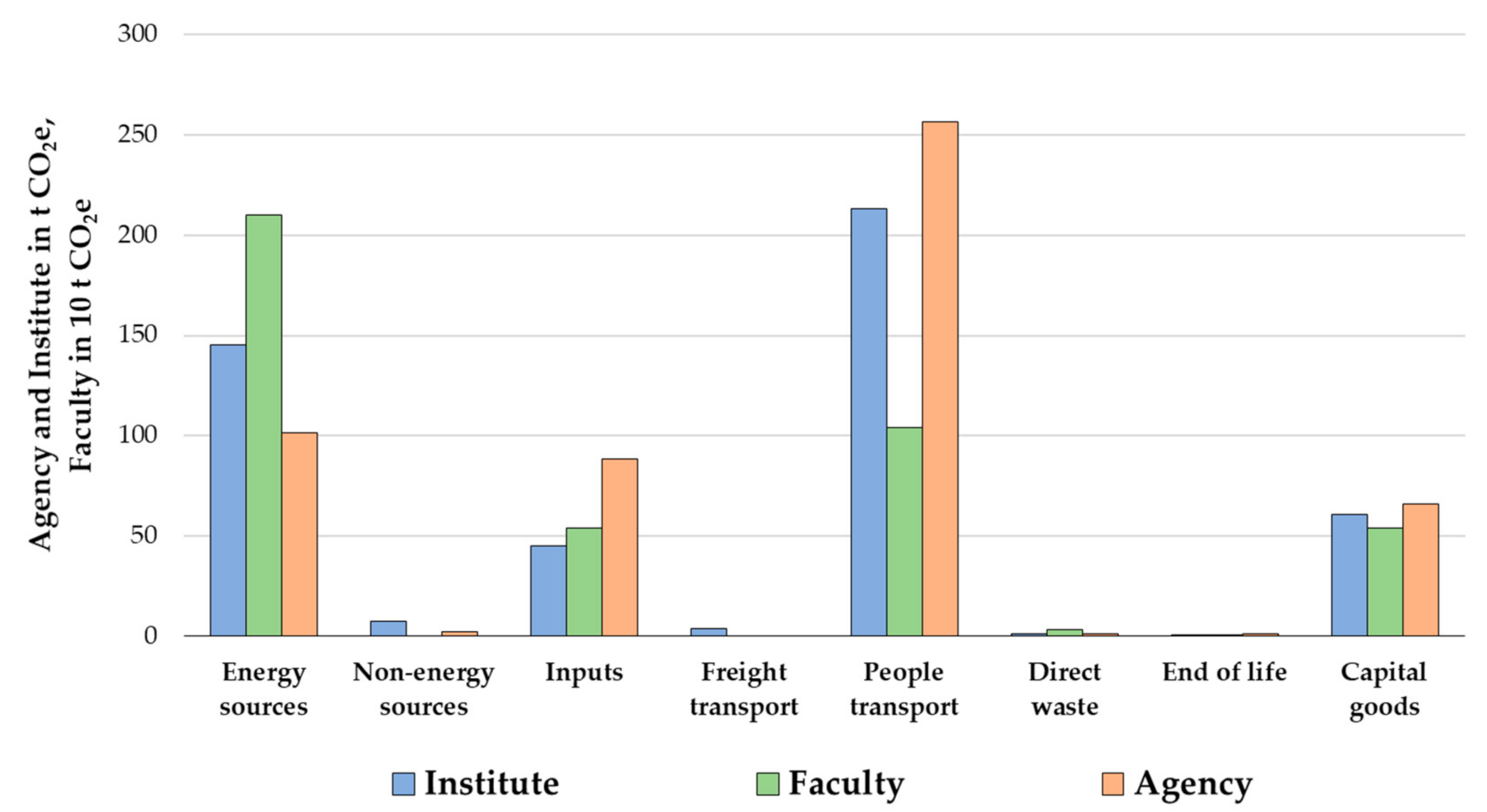
| Energy sources | 101.7 | 19.7 | 2102.0 | 49.4 | 145.2 | 30.4 |
| Non-energy sources | 2.3 | 0.4 | 0.0 | 0.0 | 7.2 | 1.5 |
| Packaging | 0.0 | 0.0 | 0.0 | 0.0 | 0.0 | 0.0 |
| Inputs | 88.2 | 17.1 | 539.3 | 12.7 | 45.1 | 9.5 |
| Freight transport | 0.0 | 0.0 | 0.0 | 0.0 | 4.0 | 0.8 |
| People transport | 256.5 | 49.7 | 1040.8 | 24.5 | 213.3 | 44.7 |
| Direct waste | 1.0 | 0.2 | 32.3 | 0.8 | 1.1 | 0.2 |
| Use of products | 0.0 | 0.0 | 0.0 | 0.0 | 0.0 | 0.0 |
| End of life | 1.1 | 0.21 | 0.6 | 0.02 | 0.1 | 0.01 |
| Capital goods | 65.8 | 12.7 | 539.6 | 12.7 | 60.9 | 12.8 |
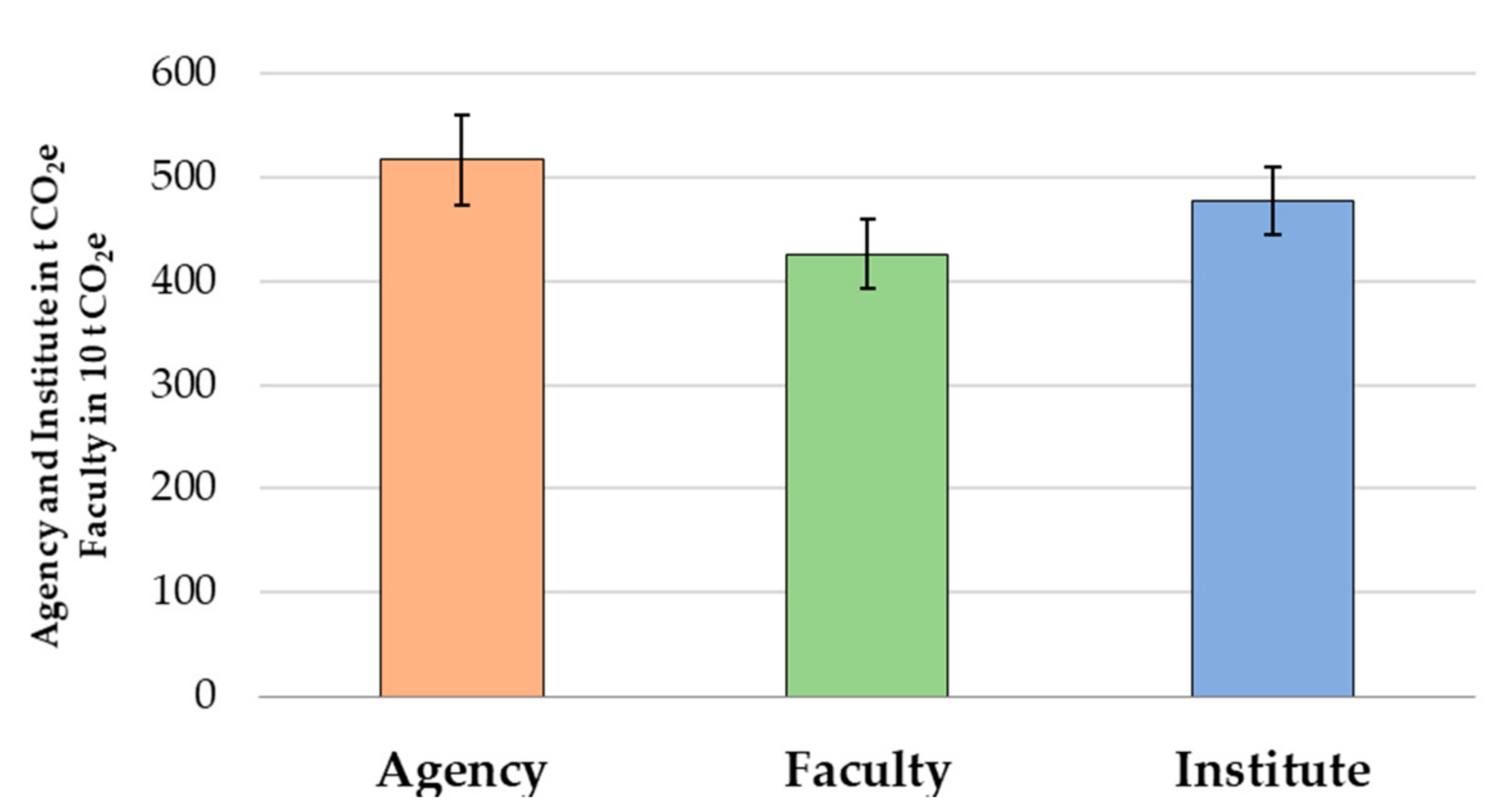
| Total CF | 516.4 | 100.0 | 4254.7 | 100.0 | 477.0 | 100.0 |
| Emission Sources/Categories/Scopes | Agency | Faculty | Institute |
|---|---|---|---|
| t CO2 e | t CO2 e | t CO2 e | |
| 1. Direct emissions from stationary combustion sources | 0.0 | 17.2 | 0.0 |
| 2. Direct emissions from mobile combustion sources | 13.5 | 4.4 | 29.2 |
| 3. Direct emissions from processes | 0.0 | 0.0 | 0.0 |
| 4. Direct fugitive emissions | 2.3 | 0.0 | 7.2 |
| 5. Direct emissions from land use, land-use change and forestry (LULUCF) | 0.0 | 0.0 | 0.0 |
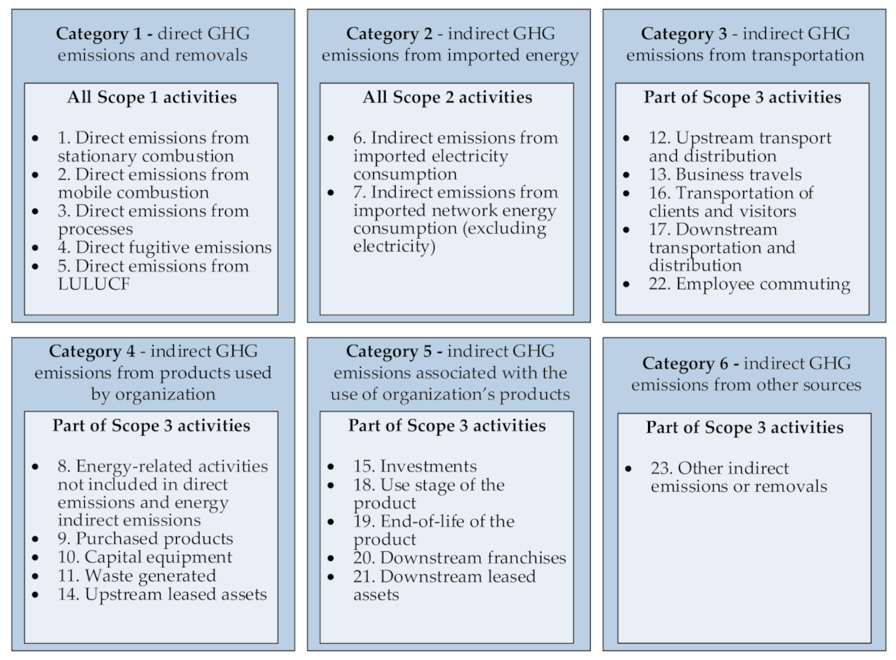
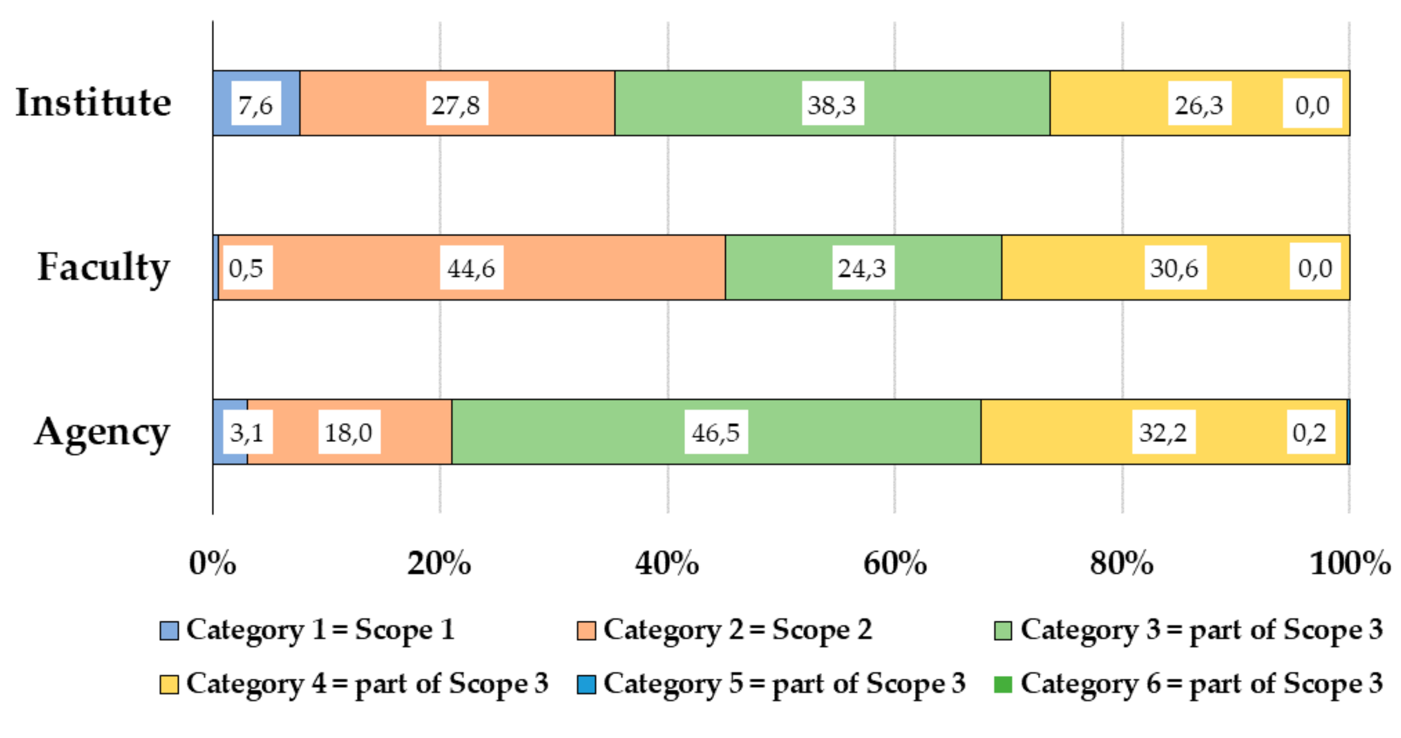
| Scope 1 = Category 1 (sources: 1–5) | 15.8 | 21.5 | 36.4 |
| 6. Indirect emissions from electricity consumption | 58.6 | 461.2 | 80.6 |
| 7. Indirect emissions from network energy consumption (excluding electricity) | 34.2 | 1435.4 | 51.9 |
| Scope 2 = Category 2 (sources: 6–7) | 92.8 | 1896.6 | 132.5 |
| 8. Emissions due to energy not covered by sources from 1 to 7 | 11.5 | 189.1 | 18.3 |
| 9. Purchased goods | 88.2 | 539.3 | 45.1 |
| 10. Capital goods | 65.8 | 539.6 | 60.9 |
| 11. Waste generated | 1.0 | 32.3 | 1.1 |
| 12. Upstream transport and distribution | 0.0 | 0.0 | 3.7 |
| 13. Business travels | 63.4 | 318.9 | 60.9 |
| 14. Upstream leased assets | 0.0 | 0.0 | 0.0 |
| 15. Investments | 0.0 | 0.0 | 0.0 |
| 16. Transportation of clients and visitors | 17.4 | 409.0 | 35.9 |
| 17. Downstream transportation of goods and distribution | 0.0 | 0.0 | 0.0 |
| 18. Use of sold products | 0.0 | 0.0 | 0.0 |
| 19. End-of-life of sold products | 1.1 | 0.6 | 0.1 |
| 20. Downstream franchises | 0.0 | 0.0 | 0.0 |
| 21. Downstream leased assets | 0.0 | 0.0 | 0.0 |
| 22. Employee commuting | 159.6 | 307.7 | 67.3 |
| 23. Other indirect emissions | 0.0 | 0.0 | 0.0 |
| Scope 3 = Categories 3+4+5+6 (sources: 8–23) | 407.8 | 2336.6 | 308.0 |
| Category 3 (sources: 12, 13, 16, 17 and 22) | 240.4 | 1035.7 | 182.5 |
| Category 4 (sources: 8, 9, 10, 11 and 14) | 166.4 | 1300.3 | 125.4 |
| Category 5 (sources: 15, 18, 19, 20 and 21) | 1.1 | 0.6 | 0.1 |
| Category 6 (source: 23) | 0.0 | 0.0 | 0.0 |
| Organization’s CF | 516.4 | 4254.7 | 477.0 |
| Organization | Result | Year | Method | Contribution of Scopes/Categories | References |
|---|---|---|---|---|---|
| Norwegian University of Science and Technology, Norway | 4.6 t CO2 e/student 16.7 t CO2 e/empl. | 2009 | GHG Protocol | Energy: 19%, Travels: 16%, Buildings: 19%, Equipment: 19% Consumables: 11%, Services 5%, Other: 10% | [29] |
| School of Forestry Engineering, Technical University of Madrid, Spain | 1.9 t CO2 e/student | 2010 | GHG Protocol | Scope 1: 8%, Scope 2: 33%, Scope 3: 59% | [40] |
| Curico campus of the University of Talca, Chile | 1.0 t CO2 e/student | 2012 | GHG Protocol | Scope 1: 16%, Scope 2: 16%, Scope 3: 68% | [30] |
| Autonomous Metropolitan University, Cuajimalpa Campus, Mexico | 1.1 t CO2 e/person 1 1.3 t CO2 e/student 5.4 t CO2 e/empl. | 2016 | GHG Protocol | Scope 1: 4%, Scope 2: 24%, Scope 3: 72% | [41] |
| Institute of Engineering at Universidad Nacional Autónoma, Mexico | 1.5 t CO2 e/person 1 | 2010 | GHG Protocol | Scope 1: 5%, Scope 2: 42%, Scope 3: 53% | [42] |
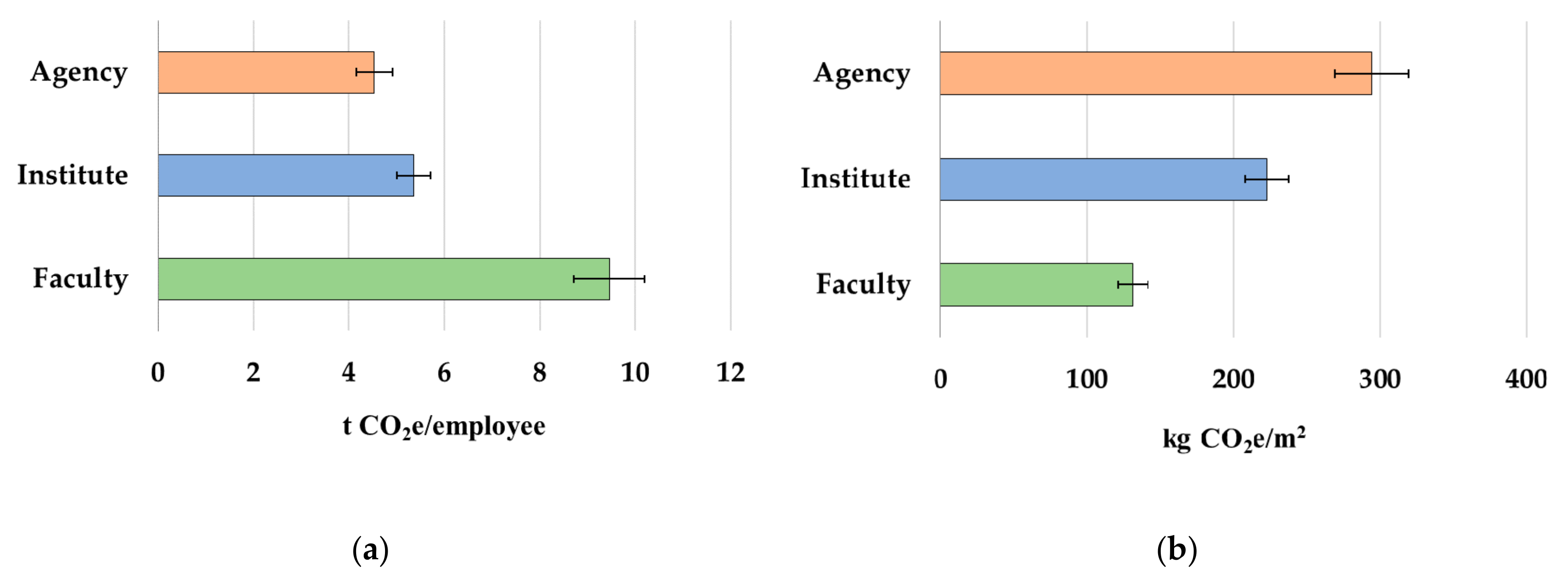
| Faculty of Mechanical Engineering and Naval Architecture, Zagreb, Croatia | 1.8 t CO2 e/student 9.4 t CO2 e/empl. | 2017 | ISO 14064-1 | Scope 1: 1%, Scope 2: 44%, Scope 3: 55% | This paper |
| Croatian Agency for the Environment and Nature, Zagreb, Croatia | 4.5 t CO2 e/empl. | 2017 | ISO 14064-1 | Scope 1: 3%, Scope 2: 18%, Scope 3: 79% | This paper |
| Energy Institute Hrvoje Požar, Zagreb, Croatia | 5.4 t CO2 e/empl. | 2017 | ISO 14064-1 | Scope 1: 8%, Scope 2: 28%, Scope 3: 65% | This paper |
| No. | Name of Measure | Description of Measure | Sub-Category | GHG Emission Reduction in 2030 (t CO2 e) | Description of the Target in 2030 | Key Monitoring Indicator |
|---|---|---|---|---|---|---|
| 1. | Eco-driving | Additional eco-driving training for new employees (training was conducted in the past) | Official cars | 1.72 | 5% reduction in official car emissions | Number of trained drivers |
| 2. | Adjusting of company fleet | Replace official cars with smaller (low power), hybrid and electric cars | Official cars | 3.45 | 10% reduction in official car emissions | Vehicle fleet renewal monitoring |
| Sub-total (Scope 1): | 5.17 | |||||
| 3. | Maintaining the internal room temperature | Maintaining the internal temperature in the room during the heating season | Heat consumption | 2.16 | 1 °C less room temperature, compared to the current temperature | Measurement and regulation of internal room temperature |
| 4. | Installation of thermostatic valves on radiators | Installation of radiator thermostatic valves to save heat energy | Heat consumption | 0.18 | Thermal energy savings: 528 kWh/a | Number of installed thermostatic radiator valves |
| 5. | Installation of the PV system | Installation of 46.4 kW (312 m2) photovoltaics on the roof of EIHP’s building | Electricity consumption | 13.74 | Electricity production: 44,291 kWh/a; electricity self-consumption: 41.771 kWh/a | Measurement of electricity production and self- consumption |
| 6. | Installation of the new chiller | Replacement of existing air-cooled compression chiller to achieve full energy efficiency of the cooling system | Electricity consumption | 0.18 | Electricity savings: 481 kWh/a | Measurement of electricity savings |
| 7. | Energy efficiency improvement of the ventilation system | Better energy efficiency can be achieved by installing recuperators in chambers and frequency converters on fan motors | Heat consumption | 3.10 | Thermal energy savings: 8857 kWh/a; electricity savings: 600 kWh/a | Measurement of electricity and heat savings |
| Electricity consumption | 0.61 | |||||
| Sub-total (Scope 2): | 19.99 | |||||
| 8. | Teleworking program | Encourage work from home among the Institute’s employees | Employee comm. by car | 26.51 | Average 2 working days from home per week | Number of working days from home |
| Other commuting | 0.41 | |||||
| 9. | Videoconferencing | Promotion of videoconferencing and virtual meetings | Business travels by plane | 21.89 | 30% reduction in business and visitor travels | Number of videoconf. and virtual meetings |
| Other business travels and visitor travels | 11.57 | |||||
| 10. | Public transportation for business travels | Promotion of transport by train or bus, instead of car or plane | Business travels | 15.12 | 10% reduction in emissions from business travels | Numbers of business travels by train and bus |
| 11. | Green public procurement | Include green requirements in the tender documentation as part of the selection criteria | Upstream transport | 0.74 | 20% reduction in emissions from paper transport | Reducing the distance for purchased papers |
| 12. | Paperless program | Promoting the paperless program and practices to reduce paper use | Purchased goods | 0.24 | 30% reduction in the number of pages of printed paper | Number of printed study pages |
| 13. | Regulator of water pressure | Installation of water pressure regulators on taps | Water consumption | 0.04 | 10% reduction in water consumption | Measuring water consumption |
| Sub-total (Scope 3): | 76.51 | |||||
| TOTAL (Scopes 1, 2 and 3): | 101.67 | |||||
| No. | Key Source Categories | GHG Emissions in 2017 (t CO2 e) | Priority Measures | GHG Emission Reduction in 2030 (t CO2 e) |
|---|---|---|---|---|
| 1. | Purchased electricity from grid | 88.13 | PV installation and energy efficiency improvement | 14.54 |
| 2. | Business travels by plane | 72.96 | Videoconferencing | 21.89 |
| 3. | Employee commuting by car | 66.26 | Teleworking program | 26.51 |
| 4. | Purchased heat from district heating | 57.11 | Energy efficiency improvement | 5.44 |
| 5. | Business travels by office car | 34.47 | Eco-driving and adjustment of company fleet | 5.17 |
| Total | 230.81 | All priority measures | 73.55 | |
Publisher’s Note: MDPI stays neutral with regard to jurisdictional claims in published maps and institutional affiliations. |
© 2020 by the authors. Licensee MDPI, Basel, Switzerland. This article is an open access article distributed under the terms and conditions of the Creative Commons Attribution (CC BY) license (http://creativecommons.org/licenses/by/4.0/).
Share and Cite
Jurić, Ž.; Ljubas, D. Comparative Assessment of Carbon Footprints of Selected Organizations: The Application of the Enhanced Bilan Carbone Model. Sustainability 2020, 12, 9618. https://doi.org/10.3390/su12229618
Jurić Ž, Ljubas D. Comparative Assessment of Carbon Footprints of Selected Organizations: The Application of the Enhanced Bilan Carbone Model. Sustainability. 2020; 12(22):9618. https://doi.org/10.3390/su12229618
Chicago/Turabian StyleJurić, Željko, and Davor Ljubas. 2020. "Comparative Assessment of Carbon Footprints of Selected Organizations: The Application of the Enhanced Bilan Carbone Model" Sustainability 12, no. 22: 9618. https://doi.org/10.3390/su12229618
APA StyleJurić, Ž., & Ljubas, D. (2020). Comparative Assessment of Carbon Footprints of Selected Organizations: The Application of the Enhanced Bilan Carbone Model. Sustainability, 12(22), 9618. https://doi.org/10.3390/su12229618