Article

Estimation of Ecological Connectivity in a City Based on Land Cover and Urban Habitat Maps

1
Department of Landscape Architecture, Graduate School of Environmental Studies, Seoul National University, Seoul 08826, Korea
2
Transdisciplinary Program in Smart City Global Convergence, Seoul National University, Seoul 08826, Korea
3
Interdisciplinary Program in Landscape Architecture, Seoul National University, Seoul 08826, Korea
*
Author to whom correspondence should be addressed.
Sustainability 2020, 12(22), 9529; https://doi.org/10.3390/su12229529
Submission received: 10 October 2020 / Revised: 9 November 2020 / Accepted: 12 November 2020 / Published: 16 November 2020

Abstract

:
Anthropogenic land use has led to the loss and fragmentation of native habitats and disruption to ecosystem processes, resulting in a decline in landscape connectivity and biodiversity. Here, in order to find the potentials of improvements in ecological connectivity, we provide a spatial analysis to present differences in ecological connectivity based on land cover maps and urban habitat maps in Suwon city, Republic of Korea. We generated two permeability maps for use in a network analysis, one being land cover and the other urban habitat, including a 5-km buffer area from the city boundary. We then determined the current-flow betweenness centrality (CFBC) for each map. Our results indicate that forests are typically the most highly connected areas in both maps. However, in the land cover map results, nearly all high-priority areas were in the mountainous region (CFBC value: 0.0100 ± 0.0028), but the urban habitat indicated that grasslands and rivers within the city also significantly contribute to connectivity (CFBC value: 0.0071 ± 0.0022). The CFBC maps developed here could be used as a reference when introducing green infrastructure in cities. Before establishing ecological networks for urban areas, future work should integrate the land use and ecological data of different administrative districts with continuous ecological connection.

1. Introduction

Expanding and intensifying anthropogenic land use has led to the loss and fragmentation of natural ecosystems, dramatic alterations in ecological functions and processes, and resultantly, a considerable decline in biodiversity [1,2,3]. In human-modified landscapes, many species inhabit more or less isolated habitat patches surrounded by a hostile or poor-quality matrix. Gene flow between populations may be disturbed by local extinction events and colonization dynamics. Changes in land use causing the disconnection have been intensively occurring in cities [4,5]. Given that 55% of the world’s population lives in cities, changes in natural dynamics due to urban land use are widespread and will likely increase, as this percentage is projected to reach 68% by 2050 [6].
Habitat fragmentations are often found in the center of cities, although the large area of green space, such as forests, tends to remain connected outside of city boundaries [7]. An uneven distribution of parks and green areas within cities not only causes inequality in accessibility for humans, but also reduces biodiversity [8,9]. In growing urban areas, green spaces are crucial for accommodating species by preserving their network or habitats [9]. Subsequently, green spaces act as a tool to prevent the loss of biodiversity by keeping gene flow among populations [9].
Landscape connectivity is defined as ‘‘the degree to which the landscape facilitates or impedes movement among resource patches’’ by Taylor et al. (1993) [10]. Similarly, With et al. (1997) defined the term as ‘‘the functional relationship among habitat patches, owing to the spatial contagion of habitat and the movement responses of organisms to landscape structure’’ [10]. Since the early 1970s, a spatial structure that affects population dynamics, an ancestor of landscape connectivity, was discussed [10]. In 1984, Merriam introduced ‘‘landscape connectivity’’ as a concept that emphasizes the effect of landscape structure on determining movement of organisms among habitat patches [10]. The necessity of corridors for movement through patches was questioned [11,12,13,14,15,16,17] by recognizing organism movements through non-habitat or matrix elements [11,18]. Then, the influence of the entire landscape was included in the conception of connectivity, and the term, landscape connectivity was defined in 1993 [9,11]. Generally, landscape connectivity promotes biodiversity of species, population, and gene flow among resource patches, at both ecological and evolutionary timescales [10]. Increasingly, conservationists suggest that maintaining or restoring landscape connectivity is crucial not only to conserve ecological integrity within cities, but also to arrest global climate change [19,20,21].
With respect to animal movement, functional connectivity is dependent on how an organism perceives and responds to the landscape at various spatial scales [3,22]. Structural connectivity can be defined based on the inter-patch distance, density, complexity, the width and quality of corridor networks, and the permeability of the landscape matrix [23,24]. Land managers and regional, national, and local governments have sought guidance from the scientific community to identify areas that should be prioritized in terms of maintaining or restoring landscape connectivity.
Based on the above, various “least-cost connectivity-related methodologies” have been developed; the least-cost path (LCP) seeks to balance habitat suitability, the minimum Euclidean distance, and the degree of connectivity between two endpoints [3,25]; the least-cost corridor (LCC) aims to optimize the connection between habitat patches [26]; the least-cost distance (LCD) uses the full surface that contains grid cell values [27,28]. In addition, circuit theory (current-flow) approaches are being developed and increasingly applied [29]. For spatial modeling, both least-cost analyses and circuit theory generate a resistance map showing landscape permeability, which represents the cost (i.e., difficulty) to the target species when moving through a given pixel [30]. Whereas the former identifies the route through which an animal may move [31], the latter identifies locations what would be used by a random walker moving between a source and target [32]. Although these approaches have proved useful in addressing specific conservation questions, broader conservation management goals require a detailed understanding of the movements of species through human-modified landscapes and how these movements are affected by habitat fragmentation and changes in matrix permeability [33,34,35]. These objectives are commonly met based on expert-derived species–habitat relationships, but these perform poorly compared to empirical movement models [3,36]. Moreover, most efforts to model landscape connectivity have focused on a limited number of focal species, which may not be representative of a region’s biota [37]. In this study, we do not consider landscape connectivity simply as the efficiency and possibility of species movement from the standpoint of urban planning, but as major basis of green infrastructure in city.
In the Republic of Korea, habitat destruction and degradation and biodiversity decline are serious issues that have arisen due to high human population density; nearly 90% of the population lives in cities [38]. Therefore, the biodiversity and ecological network of Korean cities where large populations live and, even more so, the connectivity of green patches in Korean cities are important. Generally, the green patches, especially gardens, have an environmental function, such as redeveloping empty or abandoned areas in the city [39]. Research has sought to improve various aspects of urban ecological connectivity. For example, one study focused on connectivity in urban parks as a product of the distance to forest areas and water bodies, and suggested practical solutions to improve the “green network” [40]. Urban green spaces provide a green network within cities; as an example, assessing bird movement paths within this network could lead to cost-effective methods to improve connectivity [41]. However, investigations of the practical aspects of connectivity are limited by a lack of ecological and biological information [42]. Land cover maps, typically updated every 10 years in Korea, can be useful for figuring out the state of land use in the country level to determine current land use types.
Ecological data can be added to these maps to create an urban habitat map, which can then be used to evaluate green networks at the city level. These maps would then provide more accurate information on urban connectivity and facilitate conservation and restoration planning [42]. In Korea, urban habitat maps have been developed at a 1:5000 scale since 2001, in Seoul city [43]. The Korean Government has made producing and utilizing urban habitat maps mandatory in 84 cities from 2017, and the final is due in 2021 [43]. Landscapes are classified based on environmental criteria including the distribution of floral and faunal species, land use type, and vegetation biotope. Thus, urban habitat maps provide detailed ecological information on cities and are appropriate for analyzing urban ecological networks.
We aimed to quantify differences in the ecological connectivity results produced by land cover and urban habitat maps, to identify areas that should be prioritized for conservation. Specifically, we will: (1) Assess ecological connectivity from two maps that are currently used in urban ecological planning and compare the results from two maps. (2) Then we will discuss what kind of spatial data source is practical, and how it can be practical in our study area, and (3) especially, which map more accurately reflects the values of ecological core areas such as urban streams or forests.

2. Materials and Methods

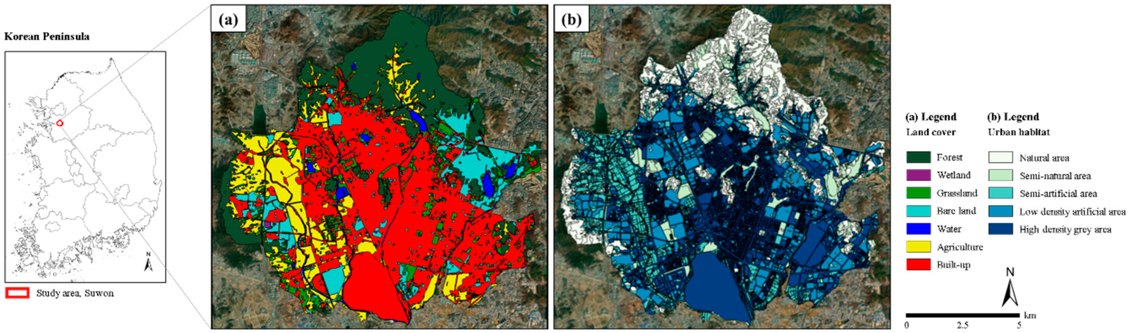
2.1. Study Area and Datasets

Our study area was located in Suwon city, Gyeonggi Province, Republic of Korea (Figure 1). Suwon is in the south-central part of Gyeonggi and covers an area of 121 km2. The city is located in a basin, with Mt. Gwangyo and Mt. Yeogi located to the north and west, respectively, and a plain located to the southeast. Forested areas are relatively well-connected on the northwest outskirts of the city. Highly fragmented urban forests and parks are located in the city center.
The land cover map used in this study was developed in 2018 and obtained from the Environmental Geographic Information Service (http://egis.me.go.kr) [44]. In connectivity analyses, it is important to consider the potential impacts of adjacent cities. Previous work has suggested that error can arise when cities are considered as isolated units—i.e., when the area adjacent to the administrative boundary is ignored. Connectivity would be underestimated with this approach. To address this, in our analysis of the ecological network of Suwon we generated a 5-km buffer from the city boundary to include the forests which are considered as targets as well as the city area to analyze the entire ecological network of Suwon.

2.2. Connectivity Analysis

We used current-flow betweenness centrality (CFBC) for the connectivity analysis. CFBC is a current-flow-based model used to identify several important pathways, including both the shortest path and alternative pathways, so it collects a network that has a more diffuse shape allowing the prioritization of unnecessary linkages [44,45]. Furthermore, it has no nodes of zero level because of random-walk performance. The current-flow method evaluates options for linking endpoints that have been determined already. A single pair of nodes was extended to all pairs in a map, and to some extent the node affects to paths or flows between all other nodes. Therefore, the map is a substitute for a set of nodes (grids) and each grid receives a weight that represents how easy it is to go through the area of the grid [45]. CFBC uses a hexagonal grid, which increases connections between cells and minimizes the distances between cell centers [46,47]. High CFBC values within a hexagon or lattice of hexagons indicate strong connectivity. We considered the degree of permeability of patches as weight values of each cell in order to develop a landscape connectivity map. Therefore, in this study, the CFBC models were computed from the permeability maps and only CFBC values within the study boundary were included in the final map product [44,45]. All statistical analyses and visualizations were completed using ArcGIS Pro software (version 2.2.0; ESRI Inc., Redlands, CA, USA). The Connectivity Analysis Toolkit was used for the CFBC analysis [45].

2.3. Generating Permeability Maps

It is appropriate to assign the weight values of permeability as an input for conducting landscape connectivity analysis (i.e., current-flow betweenness centrality analysis). Permeability normally reflects the extent to which target species move across a landscape. Here, we considered levels of natural areas (i.e., rivers, vegetation, ground permeability) as permeability rather than one of the target species. We assigned weights to the land cover and urban habitat map categories, which are shown in Figure 1 and described in Table 1 and Table 2. The former followed the method of Kang et al. (2018) [44], and the weight of the latter was given by 20 equal interval values from 1 to 100, depending on 5 defined categories of urban habitats to represent the preferred permeability each land cover type category has in the landscape (Table 1). Urban habitat types indicate relative natural value levels in a single city, so equal interval reclassification to 100 is useful. Both permeability maps had a 100 × 100 m cell size, to match the land cover map.

3. Results

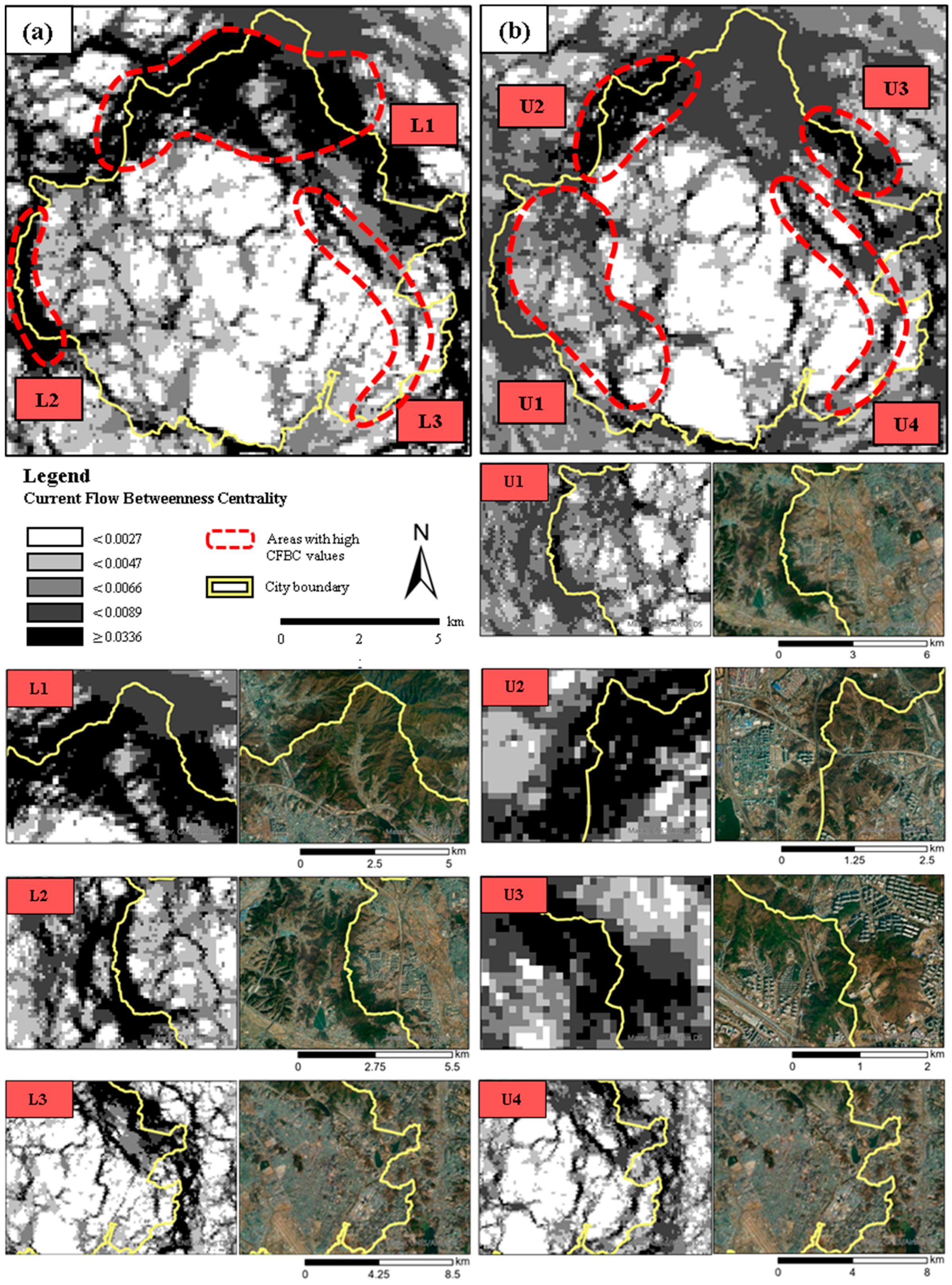
3.1. Current-Flow Betweenness Centrality Results Derived from Land Cover and Urban Habitat Maps

CFBC results are presented in Table 3 and Figure 2. The mean land cover-based CFBC value was 0.0052 ± 0.0037, and the mean urban habitat-based CFBC value was 0.0049 ± 0.0030 (Table 3). Areas of high connectivity in the northern and westerns parts of Suwon, which are mountainous, were observed in both maps, with minimal contributions from the central and southeast regions (Figure 2). Relatively high CFBC values (>0.0066) in the land cover-derived map were concentrated in the northern mountainous region. We found that fragmented forest patches and urban parks could act as corridors connecting major areas, based on their high CFBC values (Figure 2 and Figure A1), and that built-up areas rarely contributed to connectivity (CFBC < 0.0027).
Regarding the urban habitat results, mountainous and agricultural areas had high centrality values (>0.0066) (Figure 1a and Figure 2b). Specifically, agricultural areas in the west made considerable contributions to connectivity, as did mountainous areas in the northwest and northeast (Figure 1a and Figure 2b). Urban parks contributed to connectivity, linking these mountainous areas (Figure 2b and Figure A1)

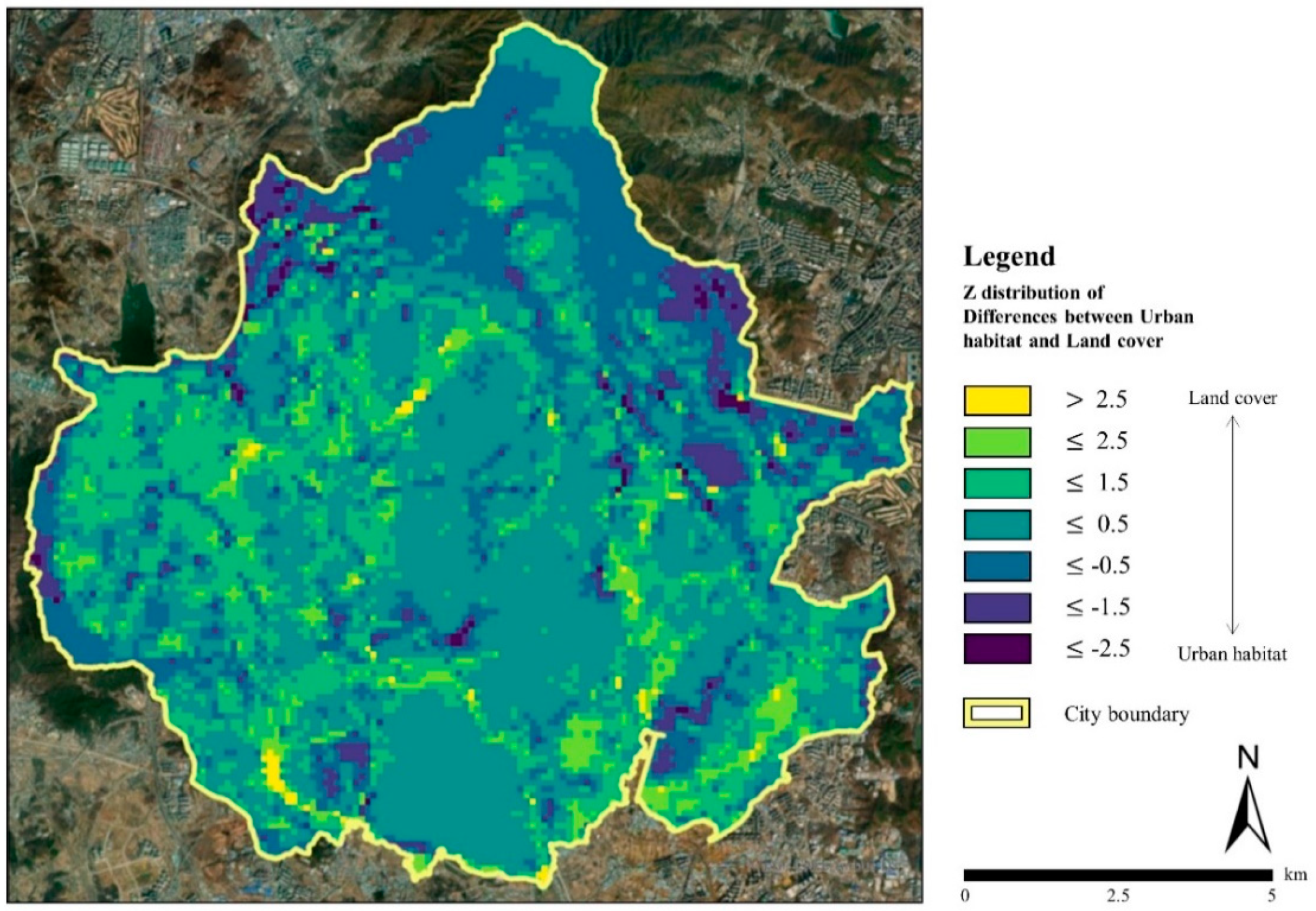
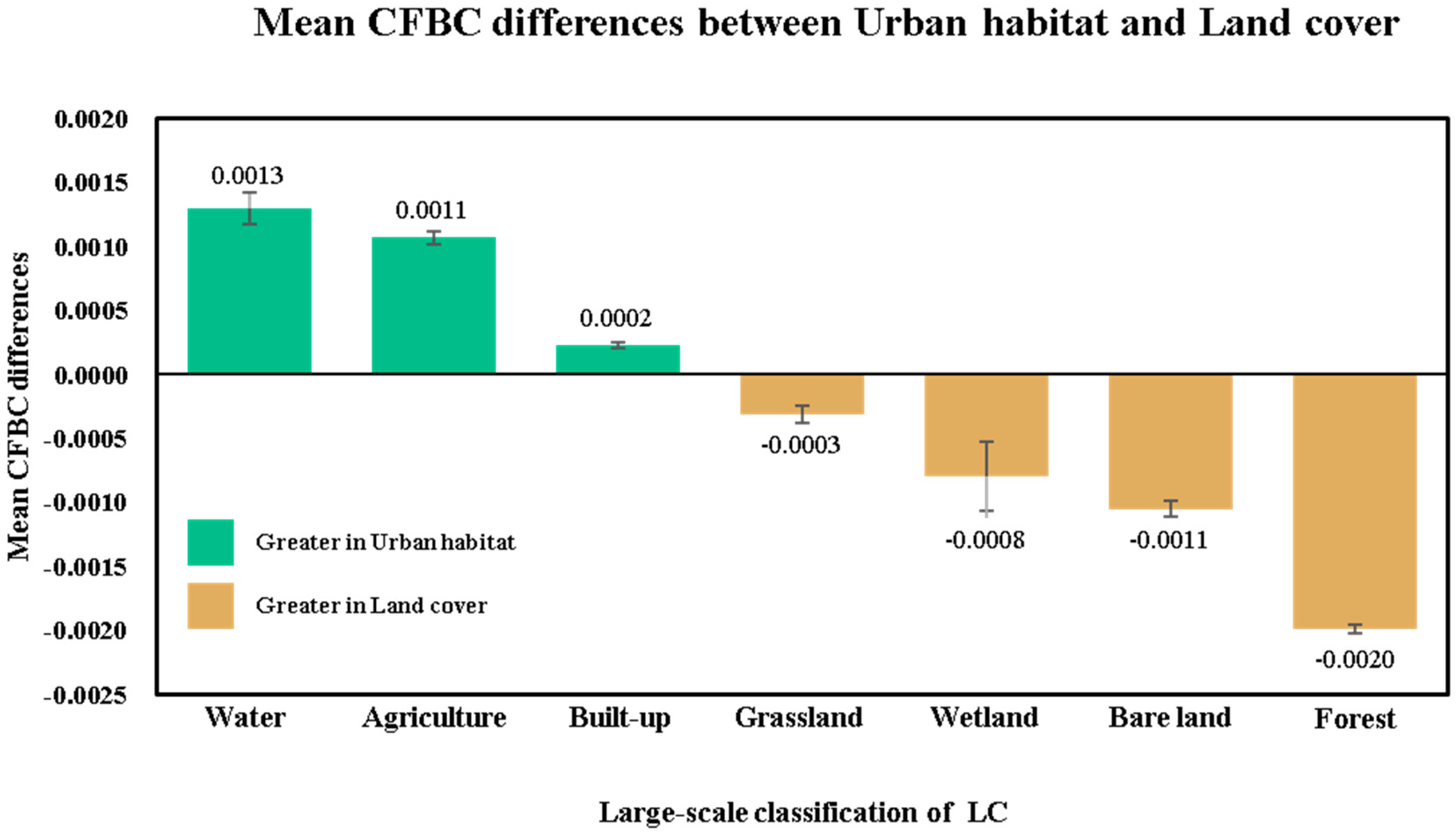
3.2. Differences between the Current-Flow Betweenness Centrality Maps

The CFBC results derived from land cover and urban habitat maps differed. First, the land cover map results indicated very high connectivity in forested areas, with other land cover types having a generally low connectivity. By contrast, the urban habitat-derived map showed a more uniform distribution of connectivity across land cover types. For example, areas with CFBC values of 0.0047–0.0066 were more widespread in the urban habitat results, but the majority of areas in the land cover map had CFBC values > 0.0336 and <0.0047 (Figure 2). Second, the spatial gradient of CFBC values was steeper in the urban habitat map relative to the land cover map, while the gradient was neither steep nor shallow within forested areas in the urban habitat map (Figure 2).
To visualize these differences, the land cover-derived CFBC values were subtracted from the urban habitat-derived values, converted into a Z-distribution, and displayed on a map (Figure 3). The mean difference in CFBC was 0.0003 ± 0.0021, indicating that the average land cover-derived values were higher than the urban habitat-derived ones (Table 3). Significant Z values were found in water, agriculture, forest, and bare land areas (Z values < |1.5|) (Figure 1 and Figure 3)—there is a similar tendency shown in Figure 4. In order to compare the contribution of urban habitat and landcover maps to ecological connectivity, the mean CFBC differences between two maps were classified depending on seven land cover types (Figure 4). Water and agricultural areas showed relatively higher connectivity in the urban habitat map, while forest and bare land showed higher connectivity in the land cover map. The mean CFBC difference values for water and agriculture in the urban habitat map were 0.0013 and 0.0011, respectively. In the land cover map, the average CFBC difference values in forest and bare land were 0.0020 and 0.0011, respectively. Generally, built-up and grassland area values were not significantly different between the two maps. The mean CFBC value of built-up was higher by 0.0002 in the urban habitat map and that for grassland was higher by 0.0003 in the land cover map.

4. Discussion

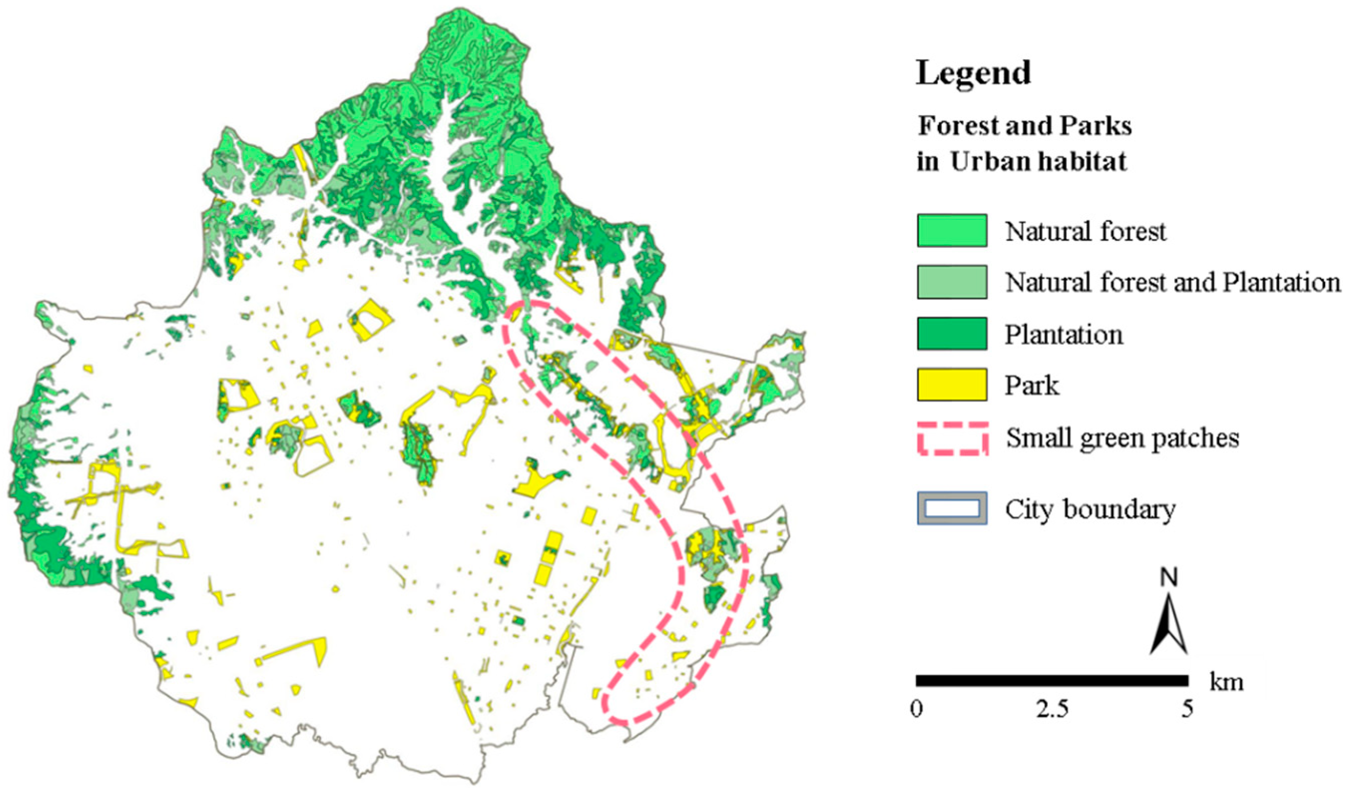
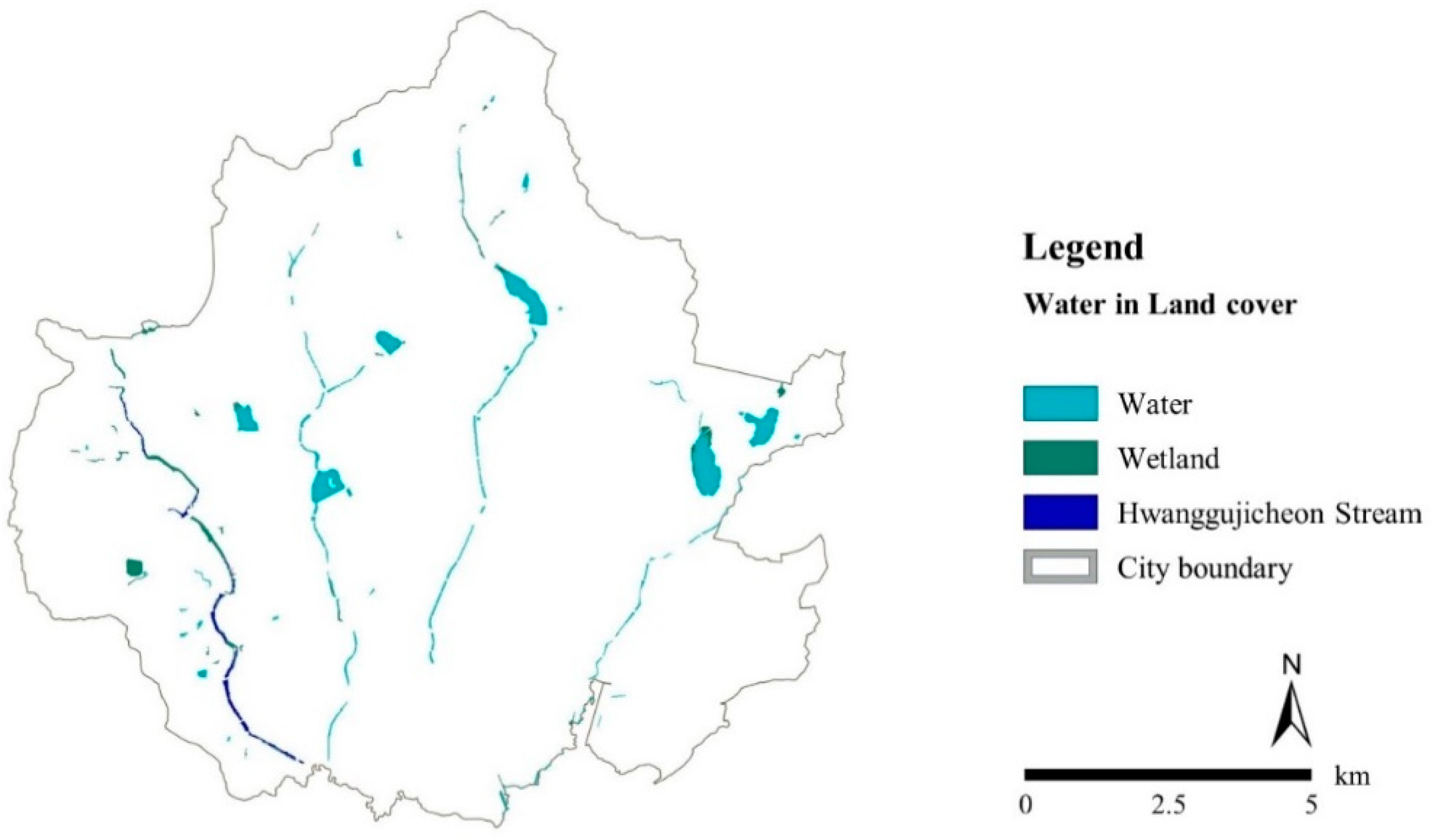
4.1. Land Cover Map and Urban Habitat Map for the Connectivity Analysis

In the Republic of Korea, land cover maps are produced to understand land use patterns at the national level, with the general aim of distinguishing developed from natural areas. Thus, urban ecological status maps compensate for this by providing more detailed ecological information. Closely, forests are classified into three types based on land cover maps, but 13 types based on urban habitat maps, with the latter providing information at a finer resolution that more accurately reflects ecological parameters and processes. Furthermore, the biotopes of urban habitat maps reflect factors such as the height of buildings, types of waterfront areas, ground impermeability, vegetation status, and river level. The five categories of the urban habitat map are thus appropriate for assessing ecological networks in cities, because they include definitions of urban spaces from an ecological perspective.

4.2. Contribution to Connectivity

The CFBC results compared with the land cover map indicated that forests, their fragmented patches, and small green patches highly contribute to ecological connectivity in Suwon. Meanwhile, the water bodies and agriculture areas also construct a connectivity of city, and have potentiality due to their extent and location. Our results indicated that forests were typically the most highly connected areas in both maps. Fragmented forest patches contributed significantly to urban connectivity in the land cover maps, as did water bodies in the urban habitat maps (Figure 1, Figure 2 and Figure 3). Furthermore, small green patches, including parks, contributed to connectivity within Suwon City (Figure 2 and Figure A1). The etymology of “Suwon”, the name of the site, is derived from water fountains and resources. Reservoirs and lakes in Suwon appear to be relatively evenly distributed and function as key connectivity corridors (Figure A2). When areas with natural resources are developed, conservation priority should be given to reservoirs and lakes. Streams are line-shaped patches that affect the interconnectivity of the matrix more than dot-shaped patches when they have the same area and make a disproportionately large contribution to connectivity due to their shape and branching structure [48]. However, we should be cautious when interpreting the results because water bodies and wetlands show spatial overlap.
We also found that agricultural areas contributed to connectivity. Currently, 14% of Suwon is agriculture land, which is concentrated in the west along the Hwanggujicheon Stream (Figure A2) that acts as bridges between mountainous and built-up areas in the city (Figure 1 and Figure 2). Within cities, agricultural areas can function as core areas for promoting ecological and biological connectivity than non-agricultural urban areas; Clucas et al. (2018) [49] showed that farmland in cities enhanced connectivity by serving as a “stepping-stone” and temporary resting place for mammals and birds. In Suwon, some agricultural areas are known habitats for endangered species, such as Hyla suweonensis [50]. However, we note that Suwon has a high proportion of built-up areas (43% of the total area) relative to cities that may be more agriculture-dominated; expansion of the built-up area needs to be carefully considered for biodiversity conservation.

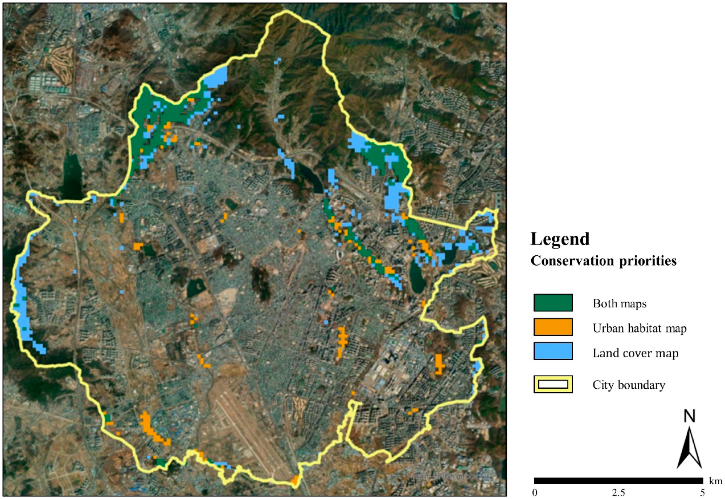
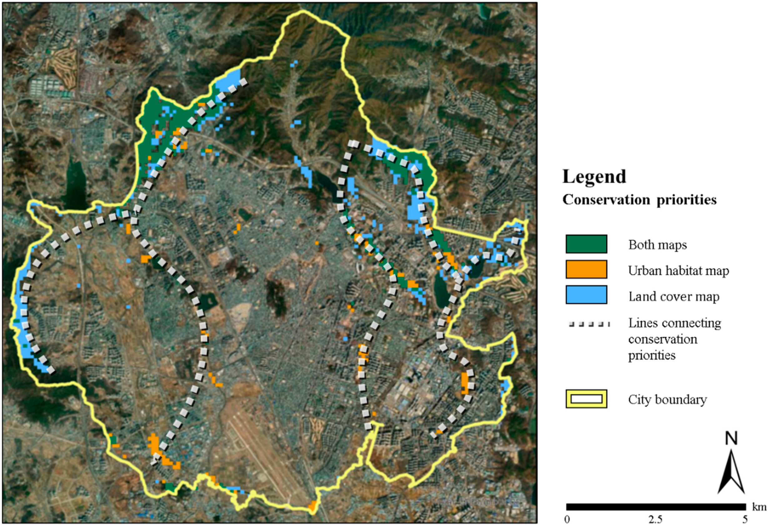
4.3. Conservation-Priority Areas

To contribute to conservation efforts in Suwon, priority areas were selected based on the CFBC Z-distribution results obtained using both maps, which allowed us to visualize the top 5% of areas in the city in terms of ecological connectivity. In Figure 5, green, orange and blue areas are those making a large contribution to connectivity in both maps, only the urban habitat map, and only the land cover map, respectively.
Areas of high-conservation priority in both maps included mountainous areas and fragmented mountain areas within the urban zone of Suwon. The large forest area in the north was not considered significant, possibly due to the valley located in the center, which may have reduced the overall connectivity in this area. In the land cover map results, nearly all high-priority areas were in the mountainous region. By contrast, the urban habitat results indicated that grasslands and rivers within the city were also important to connectivity, therefore they highlighted the important contribution of small patches within the city to the urban ecological network; their contribution was often equivalent to that of forest patches. However, the centrally located forest patches and associated lakes did not contribute significantly to connectivity in both map (Figure 5, Figure A1 and Figure A2). In spite of being located somewhere with favorable conditions, small forest patches in the center of Suwon were not significant as some of them were isolated from other patches. When it comes to landscape structural features, landscape connectivity highly relies on the average degree of patch isolation over the landscape [10]. Therefore, not only should the spatial distribution in priority conservation areas be considered for a green network plan but adjacent areas of small forest patches in the center may be critical to improving connectivity.
In order to enhance the green network in Suwon, the areas under the lines that connect conservation priorities (Figure 6, grey dot-lines) should be preferentially protected but should also be considered as prioritized zones for newly launched green patches. Especially, the agricultural area discussed in Figure 2 is surrounded by priority lines, so it has possibility to function as large mild core area relative to near urban area.

5. Conclusions

We conducted an ecological network analysis based on both land cover and urban habitat maps for Suwon, identified areas that should be prioritized for protection, and established an ecological network in the city by synthesizing the results from both maps. The results differed between the two maps, particularly for water, agricultural, bare land, and forest areas. The urban habitat map results showed that water bodies and agriculture were areas of high connectivity, while forests, bare land, and wetlands were highly connected in the land cover map.
We demonstrated that small urban green patches highly contribute to the whole ecological connectivity of cities by quantitative measurements. Especially, we identified that the level of contribution was different from types of green patches—mountainous areas and fragmented forest areas showed high-conservation priority; however, they often isolated from other patches. On the other hand, streams, line-shaped patches, largely contribute to connectivity with their branching structure. Additionally, agricultural areas in cities enhance connectivity by serving as a ”stepping-stone”. An ecological network has been planned for Suwon City to promote biodiversity. Here, we developed a CFBC map that indicates districts that primarily need to be protected for ecological connectivity in Suwon, so it could be used as a reference material when introducing green infrastructure and establishing a development plan. The method used in this study may serve as a foundation for future analysis of ecological networks by local governments that are constructing urban habitat maps. We suggest that various indicators should be weighted according to their permeability by utilizing appropriate methods. Meanwhile, these ecological network functions as a backbone to provide a variety of urban ecosystem services to citizens, in a more efficient way and at a closer distance to them. In summary, an ecological network is considered as a green infrastructure that contributes to the improvement of various ecological functions of city, even including activities such as ecosystem management of urban parks and urban gardening [51,52]. Finally, future work integrates land use and ecological data of different administrative districts with continuous ecological connections prior to establishing ecological networks for urban areas.

Author Contributions

Writing—original draft, D.K., W.S., H.C., J.K. and Y.S.; Writing—review & editing, D.K., W.S., H.C., J.K. and Y.S. All authors have read and agreed to the published version of the manuscript.

Funding

This research received no external funding.

Acknowledgments

This work was supported by the Korea Environment Industry and Technology Institute (KEITI) through the Public Technology Program based on Environmental Policy funded by the Korea Ministry of Environment (No.2018000210007). Also, this work was supported by Seoul National University through Transdisciplinary Program in Smart City Global Convergence.

Conflicts of Interest

The authors declare no conflict of interest.

Appendix A

Figure A1. Forest and parks classified by land use type.
Sustainability 12 09529 g0a1

Appendix B

Figure A2. Water features, including rivers and reservoirs, in the urban habitat type.
Sustainability 12 09529 g0a2

References

  1. Butchart, S.H.M.; Walpole, M.; Collen, B.; Van Strien, A.; Scharlemann, J.P.W.; Almond, R.E.A.; Baillie, J.E.M.; Bomhard, B.; Brown, C.; Bruno, J.; et al. Global biodiversity: Indicators of recent declines. Science 2010, 328, 1164–1168. [Google Scholar] [CrossRef]
  2. Foley, J.A.; DeFries, R.; Asner, G.P.; Barford, C.; Bonan, G.; Carpenter, S.R.; Chapin, F.S.; Coe, M.T.; Daily, G.C.; Gibbs, H.K.; et al. Global consequences of land use. Science 2005, 309, 570–574. [Google Scholar] [CrossRef] [PubMed] [Green Version]
  3. Theobald, D.M.; Reed, S.E.; Fields, K.; Soulé, M. Connecting natural landscapes using a landscape permeability model to prioritize conservation activities in the United States. Conserv. Lett. 2012, 5, 123–133. [Google Scholar] [CrossRef]
  4. Arroyo-Rodríguez, V.; Melo, F.P.; Martínez-Ramos, M.; Bongers, F.; Chazdon, R.L.; Meave, J.A.; Norden, N.; Santos, B.A.; Leal, I.R.; Tabarelli, M. Multiple successional pathways in human-modified tropical landscapes: New insights from forest succession, forest fragmentation and landscape ecology research. Biol. Rev. 2017, 92, 326–340. [Google Scholar] [CrossRef]
  5. Lindenmayer, D.B.; Fischer, J. Habitat Fragmentation and Landscape Change: An Ecological and Conservation Synthesis. Retrieved 16 September 2020; Island Press: Washington, DC, USA, 2016. [Google Scholar]
  6. United Nations, Department of Economic and Social Affairs, P.D. World Urbanization Prospects The 2014 Revision Methodology; UN: New York, NY, USA, 2014. [Google Scholar]
  7. Cui, N.; Feng, C.-C.; Wang, D.; Li, J.; Guo, L. The Effects of Rapid Urbanization on Forest Landscape Connectivity in Zhuhai City, China. Sustainability 2018, 10, 3381. [Google Scholar] [CrossRef] [Green Version]
  8. Savard, J.P.L.; Clergeau, P.; Mennechez, G. Biodiversity concepts and urban ecosystems. Landsc. Urban Plan. 2000, 48, 131–142. [Google Scholar] [CrossRef]
  9. Serret, H.; Raymond, R.; Foltête, J.C.; Clergeau, P.; Simon, L.; Machon, N. Potential contributions of green spaces at business sites to the ecological network in an urban agglomeration: The case of the Ile-de-France region, France. Landsc. Urban Plan. 2014, 131, 27–35. [Google Scholar] [CrossRef]
  10. Tischendorf, L.; Fahrig, L. On the usage and measurement of landscape connectivity. Oikos 2000, 90, 7–19. [Google Scholar] [CrossRef] [Green Version]
  11. Goodwin, B.J. Is landscape connectivity a dependent or independent variable? Landsc. Ecol. 2003, 18, 687–699. [Google Scholar] [CrossRef]
  12. Reddingius, J.; Den Boer, P.J. Simulation experiments illustrating stabilization of animal numbers by spreading of risk. Oecologia 1970, 5, 240–284. [Google Scholar] [CrossRef]
  13. Wegner, J.F.; Merriam, G. Movements by birds and small mammals between a wood and adjoining farmland habitats. J. Appl. Ecol. 1979, 16, 349–357. [Google Scholar] [CrossRef]
  14. Liro, A.; Szacki, J. Movements of field mice Apodemus ngrarius (Pallas) in a suburban mosaic of habitats. Oecologia 1987, 74, 438–440. [Google Scholar] [CrossRef] [PubMed]
  15. Potter, M.A. Movement of North Island brown kiwi (Apteryx australis mantelli) between forest remnants. N. Z. J. Ecol. 1990, 14, 17–24. [Google Scholar]
  16. Szacki, J.; Liro, A. Movements of small mammals in the heterogeneous landscape. Landsc. Ecol. 1991, 5, 219–224. [Google Scholar] [CrossRef]
  17. Johnson, A.R.; Milne, B.T.; Wiens, J.A.; Crist, T.O. Animal movements and population dynamics in heterogeneous landscapes. Landsc. Ecol. 1992, 7, 63–75. [Google Scholar] [CrossRef]
  18. Hobbs, R.J. The role of corridors in conservation: Solution or bandwagon? Trends Ecol. Evol. 1992, 7, 389–392. [Google Scholar] [CrossRef]
  19. Garcia-Lozano, C.; Varga, D.; Pintó, J.; Roig-Munar, F.X. Landscape Connectivity and Suitable Habitat Analysis for Wolves (Canis lupus L.) in the Eastern Pyrenees. Sustainability 2020, 12, 5762. [Google Scholar] [CrossRef]
  20. Worboys, G.L.; Pulsford, I. Connectivity conservation in Australian landscapes. In Report Prepared for the Australian Government Department of Sustainability, Environment, Water, Population and Communities on behalf of the State of the Environment; Australian Government Publishing Services: Canberra, Australia, 2011. [Google Scholar]
  21. Hilty, J.A.; Lidicker, W.Z., Jr.; Merenlender, A.M. Corridor Ecology: The Science and Practice of Linking Landscapes for Biodiversity Conservation; Island Press: Washington, DC, USA, 2012. [Google Scholar]
  22. Bélisle, M. Measuring landscape connectivity: The challenge of behavioral landscape ecology. Ecology 2005, 86, 1988–1995. [Google Scholar] [CrossRef] [Green Version]
  23. Baguette, M.; Van Dyck, H. Landscape connectivity and animal behavior: Functional grain as a key determinant for dispersal. Landsc. Ecol. 2007, 22, 1117–1129. [Google Scholar] [CrossRef]
  24. Metzger, J.P.; Decamps, H. The structural connectivity threshold: An hyphothesis in conservation biology at the landscape scale. Acta Oecol. 1997, 18, 1–12. [Google Scholar] [CrossRef]
  25. Walker, R.; Craighead, L. Analyzing wildlife movement corridors in Montana using GIS. In Proceedings of the 1997 ESRI User Conference, Redlands, CA, USA, 8–11 July 1997. [Google Scholar]
  26. Beier, P.; Majka, D.R.; Spencer, W.D. Forks in the road: Choices in procedures for designing wildland linkages. Conserv. Biol. 2008, 22, 836–851. [Google Scholar] [CrossRef] [PubMed]
  27. Pinto, N.; Keitt, T.H. Beyond the least-cost path: Evaluating corridor redundancy using a graph-theoretic approach. Landsc. Ecol. 2009, 24, 253–266. [Google Scholar] [CrossRef]
  28. Singleton, P.H. Landscape Permeability for Large Carnivores in Washington: A Geographic Information System Weighted-Distance and Least-Cost Corridor Assessment; US Department of Agriculture, Forest Service, Pacific Northwest Research Station: Portland, OR, USA, 2002.
  29. Rayfield, B.; Fortin, M.J.; Fall, A. Connectivity for conservation: A framework to classify network measures. Ecology 2011, 92, 847–858. [Google Scholar] [CrossRef] [PubMed]
  30. Vanthomme, H.P.A.; Nzamba, B.S.; Alonso, A.; Todd, A.F. Empirical selection between least-cost and current-flow designs for establishing wildlife corridors in Gabon. Conserv. Biol. 2019, 33, 329–338. [Google Scholar] [CrossRef] [PubMed]
  31. Adriaensen, F.; Chardon, J.P.; De Blust, G.; Swinnen, E.; Villalba, S.; Gulinck, H.; Matthysen, E. The application of “least-cost” modelling as a functional landscape model. Landsc. Urban Plan. 2003, 64, 233–247. [Google Scholar] [CrossRef]
  32. McRae, B.H.; Dickson, B.G.; Keitt, T.H.; Shah, V.B. Using circuit theory to model connectivity in ecology, evolution, and conservation. Ecology 2008, 89, 2712–2724. [Google Scholar] [CrossRef]
  33. Carvalho, F.; Carvalho, R.; Mira, A.; Beja, P. Assessing landscape functional connectivity in a forest carnivore using path selection functions. Landsc. Ecol. 2016, 31, 1021–1036. [Google Scholar] [CrossRef] [Green Version]
  34. Cushman, S.A.; Lewis, J.S.; Landguth, E.L. Evaluating the intersection of a regional wildlife connectivity network with highways. Mov. Ecol. 2013, 1, 1–11. [Google Scholar] [CrossRef] [Green Version]
  35. LaPoint, S.; Balkenhol, N.; Hale, J.; Sadler, J.; van der Ree, R. Ecological connectivity research in urban areas. Funct. Ecol. 2015, 29, 868–878. [Google Scholar] [CrossRef]
  36. Pullinger, M.G.; Johnson, C.J. Maintaining or restoring connectivity of modified landscapes: Evaluating the least-cost path model with multiple sources of ecological information. Landsc. Ecol. 2010, 25, 1547–1560. [Google Scholar] [CrossRef]
  37. Chetkiewicz, C.-L.B.; Cassady, C.; Clair, S.; Boyce, M.S. Corridors for Conservation: Integrating Pattern and Process. Annu. Rev. Org. 2006, 37, 317–342. [Google Scholar] [CrossRef] [Green Version]
  38. Choi, H.; Lee, J.; Sohn, H.; Cho, D.; Song, Y. Feasibility of Green Network in a Highly-dense Urbanized Area by Introducing Urban Gardens. Korean J. Environ. Ecol. 2017, 31, 252–265. [Google Scholar] [CrossRef]
  39. Rusciano, V.; Civero, G.; Scarpato, D. Urban gardens in the city of naples: An empirical analysis. Calitatea 2018, 19, 436–442. [Google Scholar]
  40. Hong, S.H.; Han, B.H.; Choi, S.H.; Sung, C.Y.; Lee, K.J. Planning an ecological network using the predicted movement paths of urban birds. Landsc. Ecol. Eng. 2013, 9, 165–174. [Google Scholar] [CrossRef]
  41. Sung, H.C.; Kim, M.R.; Hwang, S.Y.; Kim, S.R. A Basic Study on Connectivity of Urban Parks for the Urban Ecological Network Establishment. J. Korean Soc. Environ. Restor. Technol. 2014, 17, 125–136. [Google Scholar] [CrossRef]
  42. Park, S.C.; Han, B.H.; Park, M.J.; Yun, H.; Kim, M. A Study on the Possibility of Utilizing Both Biotope Maps and Land Cover Maps on the Calculation of the Ecological Network Indicator of City Biodiversity Index. J. Korean Inst. Landsc. Archit. 2016, 44, 73–83. [Google Scholar] [CrossRef] [Green Version]
  43. Kim, H.S.; Jang, N.R. Current Issues and Alternatives of Urban Habitat Map in Gyeonggi Province; Gyeonggi Research Institute, Ecology & Environment Lab: Suwon, Korea, 2019. [Google Scholar]
  44. Kang, W.M.; Song, Y.K.; Sung, H.C.; Lee, D.K. Assessing conservation priorities of unexecuted urban parks in Seoul using ecological network and accessibility analyses. J. Korean Soc. Environ. Restor. Technol. 2018, 21, 53–64. [Google Scholar] [CrossRef]
  45. Carroll, C.; Mcrae, B.H.; Brookes, A. Use of Linkage Mapping and Centrality Analysis Across Habitat Gradients to Conserve Connectivity of Gray Wolf Populations in Western North America. Conserv. Biol. 2012, 26, 78–87. [Google Scholar] [CrossRef]
  46. Birch, C.P.D.; Oom, S.P.; Beecham, J.A. Rectangular and hexagonal grids used for observation, experiment and simulation in ecology. Ecol. Model. 2007, 206, 347–359. [Google Scholar] [CrossRef]
  47. Rusche, K.; Reimer, M.; Stichmann, R. Mapping and assessing green infrastructure connectivity in European city regions. Sustainability 2019, 11, 1819. [Google Scholar] [CrossRef] [Green Version]
  48. Kyle McKay, S.; Schramski, J.R.; Conyngham, J.N.; Craig Fischenich, J. Assessing upstream fish passage connectivity with network analysis. Ecol. Appl. 2013, 23, 1396–1409. [Google Scholar] [CrossRef]
  49. Clucas, B.; Parker, I.D.; Feldpausch-Parker, A.M. A systematic review of the relationship between urban agriculture and biodiversity. Urban Ecosyst. 2018, 21, 635–643. [Google Scholar] [CrossRef]
  50. Song, W.K. Habitat Analysis of Hyla suweonensis in the Breeding Season Using Species Distribution Modeling. J. Korea Soc. Environ. Restor. Technol. 2015, 18, 71–82. [Google Scholar] [CrossRef] [Green Version]
  51. Rusciano, V.; Scarpato, D.; Civero, G. Territorial Social Responsibility: A Cluster Analysis on a case study. Calitatea 2019, 20, 543–548. [Google Scholar]
  52. Rusciano, V.; Civero, G.; Scarpato, D. Urban gardening as a new frontier of wellness: Case studies from the city of Naples. Int. J. Sustain. Econ. Soc. Cult. Context 2017, 13, 39–49. [Google Scholar] [CrossRef]
Figure 1. Map of Suwon, Republic of Korea (37°13′–37°21′ N, 126°56′–127°05′ E): (a) land cover classification map, with seven categories; (b) urban habitat map with five categories.
Sustainability 12 09529 g001
Figure 2. CFBC results derived from (a) land cover and (b) urban habitat maps. CFBC values in both maps are classified into five categories. L1–L3 in land cover and U1–U4 in urban habitat showed areas with high CFBC values.
Sustainability 12 09529 g002
Figure 3. Gap analysis of Z-distribution differences between the CFBC values derived from urban habitat and land cover maps.
Sustainability 12 09529 g003
Figure 4. Mean differences in CFBC values between the urban habitat and land cover-map. Results are classified by land cover type.
Sustainability 12 09529 g004
Figure 5. Conservation priority areas (both maps: Z values of both land cover and urban habitat-derived CFBC are above 1.64; urban habitat map: Z values of urban habitat-derived CFBC are above 1.64; land cover map: Z values of land cover-derived CFBC are above 1.64).
Sustainability 12 09529 g005
Figure 6. Conservation priority areas with lines connecting conservation priorities (both maps: Z values of both land cover and urban habitat-derived CFBC are above 1.64; urban habitat map: Z values of urban habitat-derived CFBC are above 1.64; land cover map: Z values of land cover-derived CFBC are above 1.64).
Sustainability 12 09529 g006
Table 1. Area in ha and proportion of total area of each land cover and urban habitat class in Suwon, Republic of Korea.
Study SiteWeight Value
Area (ha)Area (%)
Land Cover Type
Built-up5218.1543.10%1
Forest2506.5120.70%100
Agriculture1717.8714.19%10
Bare land1263.5710.44%20
Grassland1098.299.07%30
Water233.701.93%20
Wetland68.240.56%100
Total12,106.32100.00%
Urban Habitat Type
Natural area2096.1917.27%100
Semi-natural area1181.369.73%80
Semi-artificial area1932.9015.93%60
Low-density artificial area1888.5215.56%40
High-density grey area5036.7641.50%20
Total12,135.73100.00%
Table 2. Individual urban habitat types, classified by 5 levels
Level 2Definition
Natural areaForestBiotope type that absolutely needs conservation for the entire site
Semi-natural areaRiver
Lake and wetland
Grassland (natural grass area)
Biotope type that prioritizes conservation for the entire site
Semi-artificial areaCroplandBiotope type that requires conservation priority in some target areas and the remaining areas need to be divided from area that land use restriction is conducted
Low-density artificial areaProcessing facility
Manufacturing area
Special purpose area
Grassland (artificial grass area)
Landscape (green) area
Bare/ruined area
Biotope type that requires land use restrictions on some of the target land
High-density grey areaResidential area
Mixed residential area
Commercial area
Public area
Transportation facility
Biotope type requiring partial improvement
Table 3. Mean current-flow betweenness centrality (CFBC) values derived from land cover and urban habitat maps.
CategoryCurrent-Flow betweenness Centrality (mean ± SD)
Land Cover
Forest0.0100 ± 0.0028
Wetland0.0074 ± 0.0027
Grassland0.0060 ± 0.0031
Bare land0.0057 ± 0.0023
Water0.0056 ± 0.0020
Agriculture0.0051 ± 0.0022
Built-up0.0026 ± 0.0020
Mean0.0052 ± 0.0037
Urban Habitat
Natural area0.0082 ± 0.0016
Semi-natural area0.0071 ± 0.0022
Semi-artificial area0.0062 ± 0.0019
Low-density Artificial area0.0048±0.0017
High-density grey area0.0026 ± 0.0022
Mean0.0049 ± 0.0030
Publisher’s Note: MDPI stays neutral with regard to jurisdictional claims in published maps and institutional affiliations.

