Article

A Hybrid Deep Learning Model and Comparison for Wind Power Forecasting Considering Temporal-Spatial Feature Extraction

1
School of Economics and Management, North China Electric Power University, Beijing 102206, China
2
Beijing Key Laboratory of New Energy and Low-Carbon Development, North China Electric Power University, Beijing 102206, China
3
School of Management, Hebei Geo University, Shijiazhuang 050031, China
*
Author to whom correspondence should be addressed.
Sustainability 2020, 12(22), 9490; https://doi.org/10.3390/su12229490
Submission received: 15 October 2020 / Revised: 4 November 2020 / Accepted: 9 November 2020 / Published: 15 November 2020

Abstract

:
The inherent intermittency and uncertainty of wind power have brought challenges in accurate wind power output forecasting, which also cause tricky problems in the integration of wind power to the grid. In this paper, a hybrid deep learning model bidirectional long short term memory-convolutional neural network (BiLSTM-CNN) is proposed for short-term wind power forecasting. First, the grey correlation analysis is utilized to select the inputs for forecasting model; Then, the proposed hybrid model extracts multi-dimension features of inputs to predict the wind power from the temporal-spatial perspective, where the Bi-LSTM model is utilized to mine the bidirectional temporal characteristics while the convolution and pooling operations of CNN are utilized to extract the spatial characteristics from multiple input time series. Lastly, a case study is conducted to verify the superiority of the proposed model. Other deep learning models (Bi-LSTM, LSTM, CNN, LSTM-CNN, CNN-BiLSTM, CNN-LSTM) are also simulated to conduct comparison from three aspects. The results show that the BiLSTM-CNN model has the best accuracy with the lowest RMSE of 2.5492, MSE of 6.4984, MAE of 1.7344 and highest R2 of 0.9929. CNN has the fastest speed with an average computational time of 0.0741s. The hybrid model that mines the spatial feature based on the extracted temporal feature has a better performance than the model mines the temporal feature based on the extracted spatial feature.

1. Introduction

In recent years, with the shortage of fossil energy and the increasingly serious environmental problems, the scale of clean energy power generation has been expanding rapidly [1]. Wind power generation has become one of the most important renewable energy generation methods due to its clean, economical and sustainable advantages [2]. By the end of 2019, the total capacity for wind energy globally is over 651 GW, 60.4 GW of wind energy capacity was installed globally in 2019 [3]. Although the wind power generation technology is becoming more and more mature, the stability, safety and economics of the wind power as well as power grid are affected due to its intermittency, randomness and uncertainty of wind power generation [4]. At the same time, the uncertainty of wind power generation power will also have impacts on the design of power markets, planning and deployment of wind power systems, power grid dispatch, transmission capacity upgrades and other issues [4]. Therefore, the accurate and effective wind power prediction technology is indispensable and of great significance for the safe, stable and economic operation.
Currently, comprehensive research on wind power forecasting methodologies has been done by numerous scholars around the world. According to different forecasting principles, wind power forecasting methods can be summarized into three main categories: physical model, statistical model and machine learning model [5,6]. Among these methods, the physical model relies on the weather and wind speed information from numerical weather prediction (NWP), which requires big data modeling. This method is suitable for long-term prediction on a large scale and is not applicable in small areas and short-term forecasting [7]. Statistical methods make predication based on spatial and temporal analysis of research data, mainly including Kalman filter (KF) [8], regression methods [9,10], exponential smoothing methods [11] and time series analysis methods [12]. Although the statistical models perform well in simple time series prediction and short-term prediction, it is insufficient in nonlinear data processing and can accumulate errors in long-term prediction [13]. Generally, statistical methods outperform physical models in short-term wind power forecasting [6].
With the development of artificial intelligence, machine learning shows a better performance in processing non-stationary wind energy sequences along with its strong robustness and effectiveness, which attracts extensive attention. The most commonly used machine learning methods include: back-propagation neural networks (BPNN) [14], support vector machine (SVM) [15], decision tree [16], radial base function neural network (RBFNN) and so on. Among them, the neural network model is most frequently used in the current wind power output time series forecasting problems [17]. Compared with physical and statistical approaches, the machine learning forecasting method can attain higher accuracy and better extraction of the wind power variation characteristics, especially when the curve of wind output fluctuates drastically [14]. Li et al. proposed an improved dragonfly algorithm optimized support vector machine (IDA-SVM) model for short-term wind power forecasting and the predicted results show that the IDA-SVM has better prediction accuracy in comparison with BPNN and Gaussian process regression [18]. Liu et al. proposed an optimized SVM model based on Jaya algorithm (Jaya-SVM) to predict the wind speed in the short-term. The validity, reliability and accuracy of the proposed model were tested through experimental calculation [19]. Wang et al. came up with a hybrid forecasting approach based on multiple machine learners (BPNN, RBFNN and SVM) combined with an ensemble learning method to predict the wind power with different weather conditions and the simulation and experiments proved its effectiveness and high accuracy [20]. Rodríguez et al. proposed an efficient forecasting method based on artificial intelligence for the very short-term (10 min) prediction of wind power density for a micro-grid, which improved the micro-grid control [21].
Although some improved machine learning methods have already achieved good performance and high accuracy, it still has difficulties in processing large bulks of input data and dealing with vanishing or exploding gradients problems. Therefore, the deep learning method has been applied in forecasting to overcome these insufficiencies. The commonly utilized deep learning methods have different categories, such as deep belief network (DBN) [22], convolutional neural network (CNN) [23], bidirectional long short time memory neural network (Bi-LSTM) [24], generative adversarial networks (GAN) [25], deep residual learning (DRL) [26]. Among them, the CNN model has already been applied in the prediction of photovoltaic power output [27], short-term load forecasting [28], wind speed and solar radiation forecasting [29]. However, there is limited research on CNN application in wind power output forecasting. Hong et al. came up with a hybrid deep learning model based on CNN cascaded with a radial basis function neural network to predict one day ahead wind power output and used a real wind farm to implement an experiment. The result showed that the hybrid deep learning method has a better performance compared with traditional methods [30]. The characteristic of sparse connection and parameter sharing feature enables CNN to have less training parameters and shorter training time as well as improve the prediction efficiency.
However, the CNN model is initially proposed for image processing, which is more suitable for processing 2D information. The transformation of information from 1D to 2D increases the model complexity and decreases the modeling accuracy [27]. Compared with the CNN model, the LSTM model is more competent at solving time series problems for its sequential data processing ability. Some research papers have utilized the LSTM model and various improved LSTM methods in irradiance forecasting, photovoltaic power output forecasting and so on. Qing and Niu [31] proposed an LSTM model for one hour ahead, one day ahead of solar irradiance forecasting and the prediction performance is compared with the persistence algorithm, linear least squares regression and back propagation neural networks algorithm, the results showed that the LSTM has a good fitting and generalization ability and higher prediction accuracy. Gao et al. [32] applied the advanced forecasting model of LSTM network for photovoltaic power generation prediction and proposed different forecasting methods for different weather and seasonal conditions. The results showed that compared with other algorithms (BPNN, WN network and LSSVM), the accuracy of output power prediction is improved. Although LSTM is superior to traditional machine learning methods in processing large bulk of input data and have a relatively fast computational speed, LSTM is not always the best choice considering the accuracy of model predictions [27,33]. Therefore, there are no intelligent algorithms or models that are competent for all problems and deep learning models cannot be spared as well. There is still room for the improvement of deep learning models in wind forecasting.
In order to overcome the shortcomings of single LSTM or CNN model and combine the advantages of them to get a better prediction effect, hybrid models based on LSTM and CNN are proposed in different areas [34]. Taking the hybrid model of CNN and LSTM as an example, Wang et al. [35] came up with an online reliability time series prediction method based on deep learning models CNN and LSTM. The proposed model can process large-scale data, as well as predict online reliability time series data effectively and accurately. Bao et al. [36] proposed a spatio-temporal deep learning architecture to predict the citywide short-term crash risk, by employing the CNN to capture the spatial dependencies and applying the LSTM neural network to capture the temporal dependency, finally, developing convolutional long short-term memory neural network (ConvLSTM) to capture the spatio-temporal features. The results showed that the proposed approach outperforms other models. Wen et al. [37] proposed a spatio-temporal convolutional long short-term memory neural network extended (C-LSTME) model to encompass the spatiality and temporality of the air quality data and integrated meteorological data and aerosol data for predicting air quality concentration. The results showed that the performance of the present model has been improved. Liu et al. [38] used wavelet transform algorithm to decompose the original data into two kinds of data with different frequencies, then utilize CNN to extract the feature from high-frequency data and LSTM to extract the feature from low-frequency data. Compared with other machine learning models (SVM, BPNN, GRNN, etc.), the performance of the hybrid model was verified, including the accuracy and robustness in wind speed forecasting. Therefore, it can be concluded that the combination of CNN and LSTM model to respectively capture the spatial dependencies and temporal dependencies has its unique advantage in solving the forecasting problem with a bulk of data characterized by temporal and spatial correlation features.
Through the above literature review, the current difficulty and research gaps of wind power generation forecasting can be summarized as follows:
  • The inherent intermittency and uncertainty of wind power lead to difficulties in accurate and rapid wind power output forecasting.
  • Few research has paid attention to the bidirectional learning feature of Bi-LSTM in the application of wind power forecasting while more research has been focused on LSTM by far.
  • To our best knowledge, the hybrid model BiLSTM-CNN has not yet been applied in the application of wind power forecasting along with the two-way time feature learning and spatial feature extraction analysis.
  • Comparison and evaluation among various deep learning models (CNN, LSTM, Bi-LSTM) and their hybrid models in wind power forecasting area have not been systematically researched.
Therefore, to overcome the obstacles and fill in the gaps described above, a hybrid model BiLSTM-CNN is proposed in this paper to forecast the short term wind power output by better taking advantage of the bidirectional temporal feature mining of Bi-LSTM and spatial feature mining ability of CNN. Grey correlation analysis under two different normalization methods is applied to determine the optimal inputs with high correlation degrees. Besides, a real wind farm in Beijing is set as a case study and implemented with experiments to verify the effectiveness and accuracy of the proposed model. Lastly, a comparison among the proposed model and other single or hybrid deep learning models(LSTM, BiLSTM, CNN, LSTM-CNN, CNN-BiLSTM, CNN-LSTM) is conducted in multiple aspects and the order to extract temporal or spatial feature is also studied.
  • Through grey correlation analysis under two different normalization methods, multiple wind speed time series data with different heights are selected as inputs of the proposed model. Through this step, the calculation complexity and time are reduced.
  • The BiLSTM-CNN algorithm is innovatively proposed in this research, which can extract time and space features in succession to fully mine the information among the input data and obtain high prediction accuracy. The contribution of this proposed model fills in the research gaps. With the experiment conducted in a real wind farm as a case study, the performance of the proposed model is verified by comparison with other single and hybrid deep learning models.
  • Model comparison among different deep learning models (LSTM, BiLSTM, CNN, BiLSTM-CNN, LSTM-CNN, CNN-BiLSTM, CNN-LSTM) are systematically studied in wind power forecasting. Three sets of comparison are conducted. Specifically, the role of the introduction of CNN to extract the spatial features among multiple wind speed series with different height is studied; the comparison between Bi-LSTM and LSTM is also studied to verify the significance bidirectional temporal feature extraction ability of Bi-LSTM; Besides, the comparison of BiLSTM-CNN vs. CNN-BiLSTM and LSTM-CNN vs. CNN-LSTM is also experimented to study the preference between ‘‘the temporal characteristics of time series are extracted in the beginning and later the spatial characteristics are extracted’ and ‘the spatial characteristics of time series are extracted in the beginning and later the temporal characteristics are extracted’.
The structure of this paper is summarized as follows.
The first section introduces the topic and problem to be solved in this paper through the literature review and briefly summarizes the current gaps and obstacles in the wind power forecasting area; The second section expounds the methodology, proposed model and the whole framework of this paper; The third section conducts a case study with data of a real wind farm in Beijing and various deep learning models are simulated to verify the performance of the proposed model as well as conduct comparison from different aspects. In addition, in order to verify the validity and reliability of the model, this chapter adds a section of further study. In further study, the data input model of a wind farm in Shanxi province with a time span of one year is expected to be selected for simulation again and the prediction accuracy of each model is compared again. The last section concludes this paper and proposes potential research idea.

2. Methodology

2.1. Grey Correlation Analysis

Many factors can cause fluctuations in wind power generation. In order to improve the efficiency and accuracy of wind power generation power prediction, it is necessary to screen the factors of input prediction model. Using grey relational analysis, several important variables can be identified from many variables to accurately predict wind power. The basic idea of the grey correlation analysis is to determine whether the different sequences have close correlation according to the grey correlation degree of the sequence geometric shape. A grey correlation degree is a method to study the degree of correlation between each factor in the system and a given factor. The stronger the correlation between the two factors is, the greater the calculated correlation coefficient will be and the inverse is also true [39,40]. The process of the model is as follows.
Step 1: Setting of the reference sequence X 0 = ( X 01 , X 02 , , X 0 N ) , the at the Wind power generation. Assuming there are m series of factors and the i t h series can be denoted as X i = ( X i 1 , X i 2 , , X i N ) , i = 1 , 2 , , n , The data sequence is shown in Formula (1).
( X 1 , X 2 , , X m ) = [ x 01 x 11 x m 1 x 02 x 12 x 11 x 0 N x 1 N x m N ]
Step 2: The reference and comparison sequences are then standardized. There are two normalization methods adopted, namely, average normalization and difference normalization, to transform the matrix into the following matrix and transforms the matrix into the following matrix.
( X 1 , X 2 , , X m ) = [ x 01 x 11 x m 1 x 02 x 12 x 11 x 0 N x 1 N x m N ]
Step 3: The absolute value difference between the corresponding element in the reference sequence and the comparison sequence is calculated.
Δ max = max i   max k { Δ 0 i ( k ) } ( i = 1 , 2 , , m ; k = 1 , 2 , , n ) Δ min = min i   min k { Δ 0 i ( k ) } ( i = 1 , 2 , , m ; k = 1 , 2 , , n )
where Δ 0 i ( k ) = | x i ( k ) Δ 0 ( k ) | ( i = 1 , 2 , , m )
Step 4: Calculate the discrete coefficient, which can show the degree of correlation:
ξ 0 i ( k ) = Δ min + ρ Δ max Δ 0 i ( k ) + ρ Δ max ,
where ρ ( 0 , 1 ) is the distinguish coefficient. Commonly, ρ = 0.5 is used [40].
Step 5: After obtaining the correlation coefficient through Formula (4), the average of gray correlation is usually used as the degree of gray correlation.

2.2. Proposed Hybrid Model

2.2.1. CNN Model

Convolutional neural networks (CNN) are feed-forward neural networks with two features of parameter sharing and sparse connecting, which can effectively capture characteristics of original data [41] CNN has good image processing performance and is a classic model of deep learning applied to image data classification and recognition. Some researchers now use one-dimensional CNNs to process sequence data. Compared to traditional neural networks, it introduces convolutional layers and pooling layers. The input data is compressed and important features are extracted through the convolution operation. And the Max-pooling layer aims to reduce the size of the feature map to grasp features and diminish the computational cost. Figure 1 shows the structure of CNN:
The convolutional layer convolves with the input feature and generates feature maps through filter. The convolution operation can be represented as:
f = φ ( u * k + b ) ,
where f , k , u and * are the obtained feature map, convolution kernel, input features and the convolution operator, respectively. The bias and activation function are represented by b and φ . The activation function plays a non-linear mapping role in the multilayer neural network, which can establish a complex functional relationship between the predicted value and the spatial-temporal characteristics of historical wind data. As shown in Formula (4), we select the RuLE function as the activation function:
g ( x ) = { x ,   i f   x > 0 0 ,   o t h e r w i s e

2.2.2. Bi-LSTM Model

(1)
LSTM Model
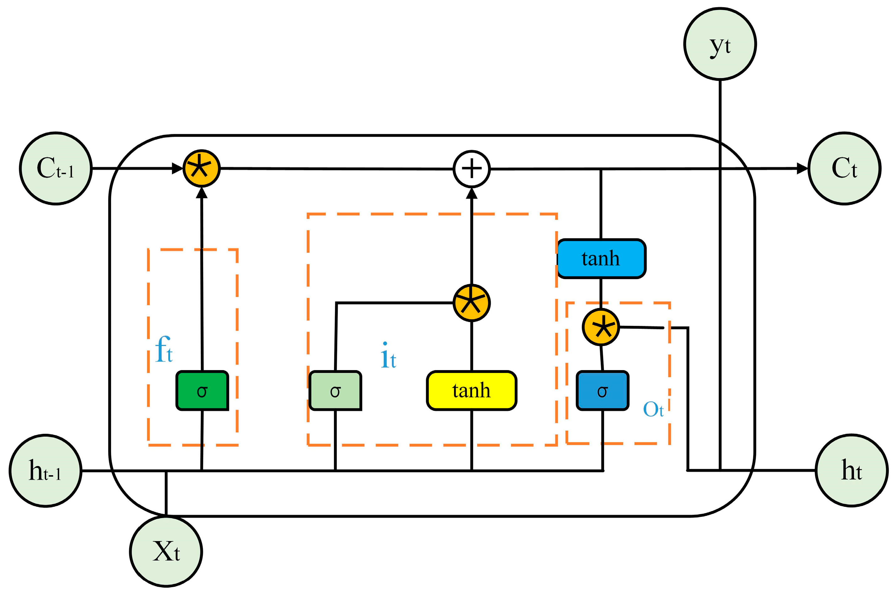
In the process of internal learning and training of traditional RNN, there will be a phenomenon of gradient disappearance and explosion, which makes it difficult for the model to train efficiently. To overcome this shortcoming, Hochreiter and Schmidhuber proposed a recurrent neural network in 1997, namely Long Short-Term Memory (LSTM) model [24]. The inherent storage unit and gate mechanism of LSTM effectively solve the defects of the RNN neural network model and save the delay event in the time series and the past information is effectively used to forecast [42]. LSTM is mainly composed of three threshold unit modules, which are divided into forget gate, input gate and output gate, its unit structure is shown in Figure 2. The LSTM model processes time series data from left to right in turn. The control switch of forget gate is used to determine the proportion of valuable information. The update process of cell unit depends on the input of the current moment, the output of the previous time and the historical memory information. The cell gets the current time information through the output gate. The information update status of cells and gates is shown in Formulas (7)–(12).
f t = σ ( W f [ h t 1 , x t ] + b f )
i t = σ ( W i [ h t 1 , x t ] + b i )
g t = tanh ( W g [ h t 1 , x t ] + b g )
c t = f t * c t 1 + i t * g t
o t = σ ( W o [ h t 1 , x t ] + b o )
h t = o t * tanh ( c t ) ,
where f t , i t , g t , o t are respectively the output values of forget gate, input gate, update gate and output gate. In the LSTM model, the output value h t 1 at time t 1 of the LSTM and the input value x t at the current time are the inputs of the four gates. W f , i , g , o and W f , i , g , o represent the weight matrix and preference vector. c t is memory unit, and σ is the sigmoid incentive function.
(2)
Bi-LSTM Model
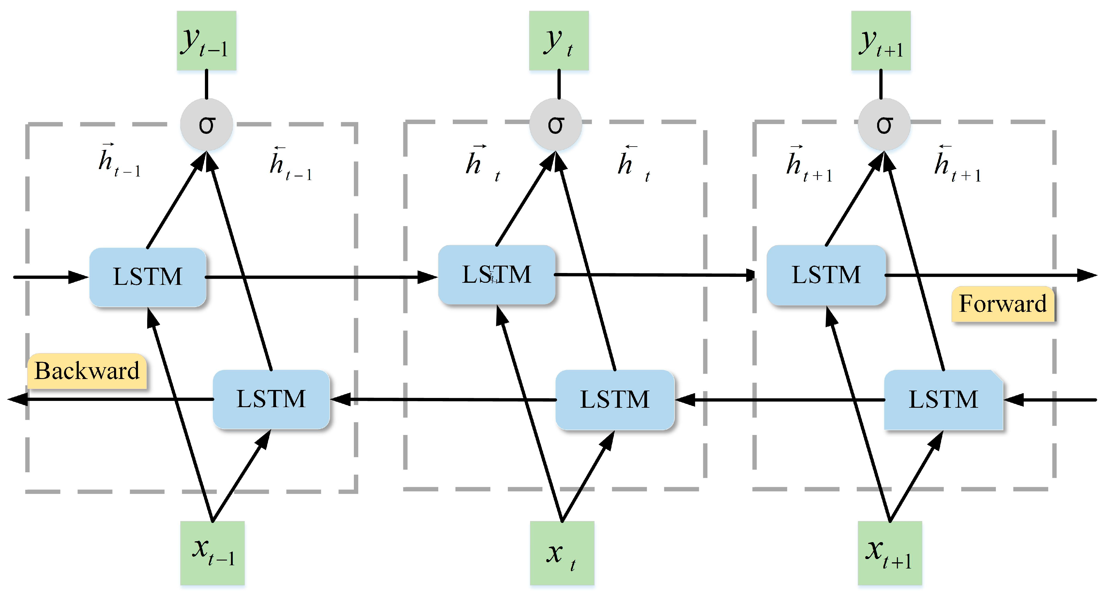
The unidirectional LSTM model uses the previous information to predict the follow-up information and the bidirectional LSTM (Bi-LSTM) improves the prediction accuracy by combining the forward and backward information of the input sequence on the basis of the LSTM [43]. For the output of a certain time, the forward LSTM layer has the information of the input sequence at that time and before and the backward LSTM layer has the information of the input sequence at that time and after. The output vectors by two LSTM layers can be processed by adding, averaging or linking. The horizontal direction simultaneously calculates the forward LSTM hidden vector h t and the reverse LSTM hidden vector h t for each time step t and the vertical direction represents the unidirectional flow from the input layer to the hidden layer and then to the output layer. This paper uses the method of connecting two hidden states to obtain the final prediction result of the Bi-LSTM model, as shown in Formulas (13)–(15).
h t = L S T M ( x t , h t 1 )
h t = L S T M ( x t , h t + 1 )
y t = W h y h t + W h y h t + b y
where L S T M ( ) represents LSTM function, W h y and W h y are the weight of forward LSTM and the weight of backward LSTM, respectively and the bias of the output layer is represented by b y .The network structure of BI-LSTM is shown in Figure 3

2.2.3. Hybrid Model

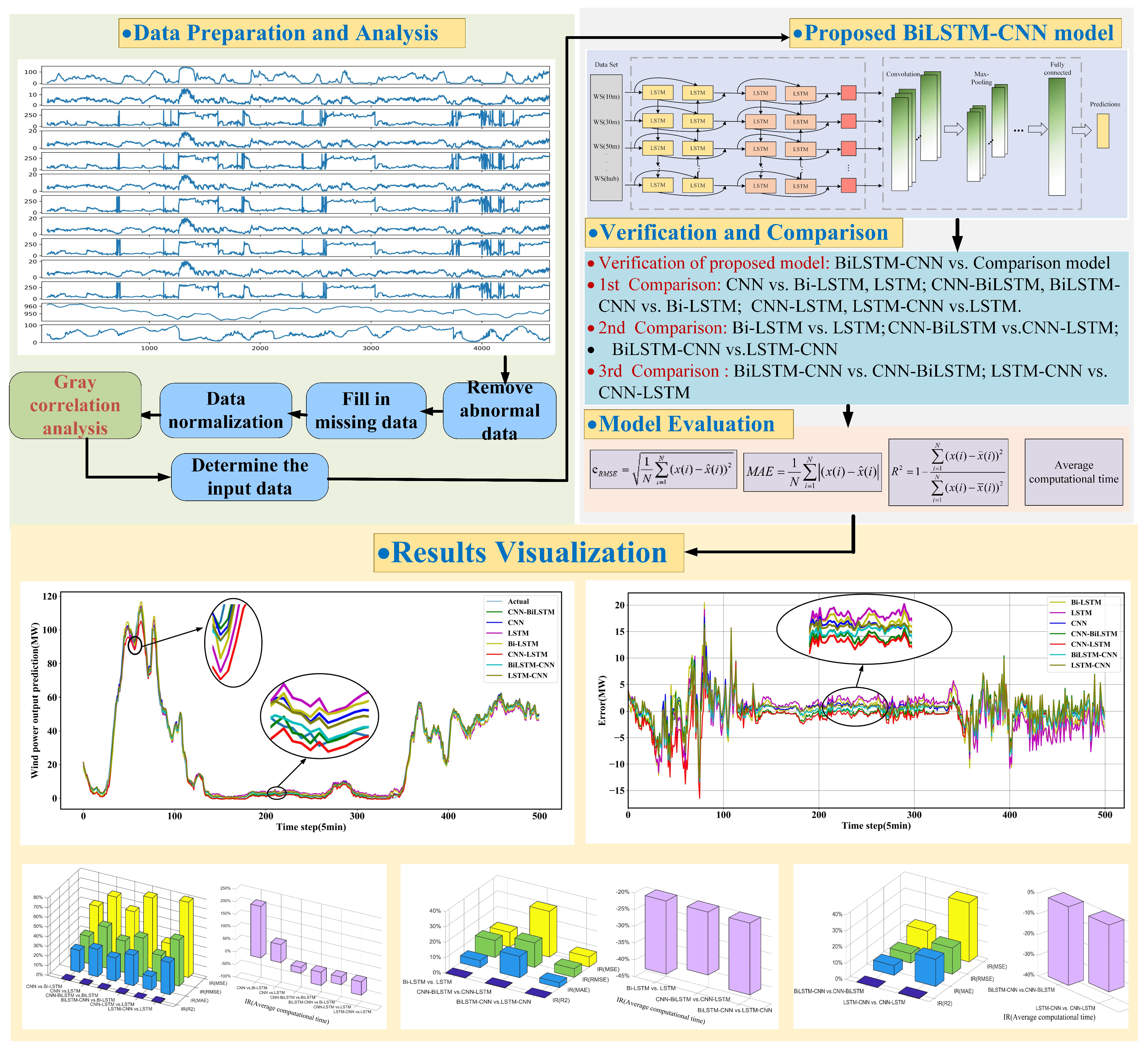
The purpose of this article is to predict wind power based on better robustness and accuracy. According to the above analysis, both BiLSTM and CNN have their unique advantages. Bi-LSTM can learn long-term temporal dependencies in bidirectional ways while CNN can better mine time-invariant spatial features of data. Therefore, a hybrid model based on Bi-LSTM and CNN is proposed to learn the temporal and spatial features among the data to better predict the short-term wind power output. In the mixed BiLSTM-CNN model, the upper model is Bi-LSTM learning temporal dependencies, while the lower model is CNN- mining time-invariant spatial features of data. The structure of the proposed model is shown in Figure 4. The framework of the case study is shown in Figure 5.
Step1: Data preparation and analysis. Before the data is input to the model, in order to improve the prediction accuracy and efficiency, it is necessary to preprocess and filter the data to improve the quality of the model input data. The preprocessing includes removing abnormal data, filling the missing values and normalizing the data. In the data screening, the grey correlation analysis method in Section 2.1 is used to calculate the grey correlation coefficient between the output wind energy data and the input impact factor data. Finally, the input index of the model is determined according to the results of the grey correlation analysis. The indicators of the original data set include historical wind power output (WP), wind speed (WS) and wind direction (WD) with different heights (30 m, 50 m, 70 m, hub height), relative humidity (H), rainfall (R) and pressure (P).
Step2: Short term wind forecasting with temporal-spatial feature extraction based on the proposed BiLSTM-CNN model. (1) Temporal feature selection based on the Bi-LSTM model. Input the filtered index data into the Bi-LSTM model and set up a two-layer neural network for time series feature extraction, where Units = 64; Units = 128. (2) Extract spatial sequence features by the CNN model. The data extracted after the noise reduction of the Bi-LSTM model is input into the CNN model to further extract the spatial characteristics of the data set through the convolutional layer and pooling layer. In the CNN model, a convolutional neural network including 2 convolutional layers and 2 pooling layer is built for spatial feature extraction based on the extracted output of the Bi-LSTM model. The kernel size used in the convolutional layer is 3 × 3. The batch size and the learning rate of the proposed model are 100 and 0.001 respectively. Besides, to prevent over-fitting of the model, we also added the drop-out mechanism to the model. Finally, the short-term wind power prediction result is output through the fully connected layer.
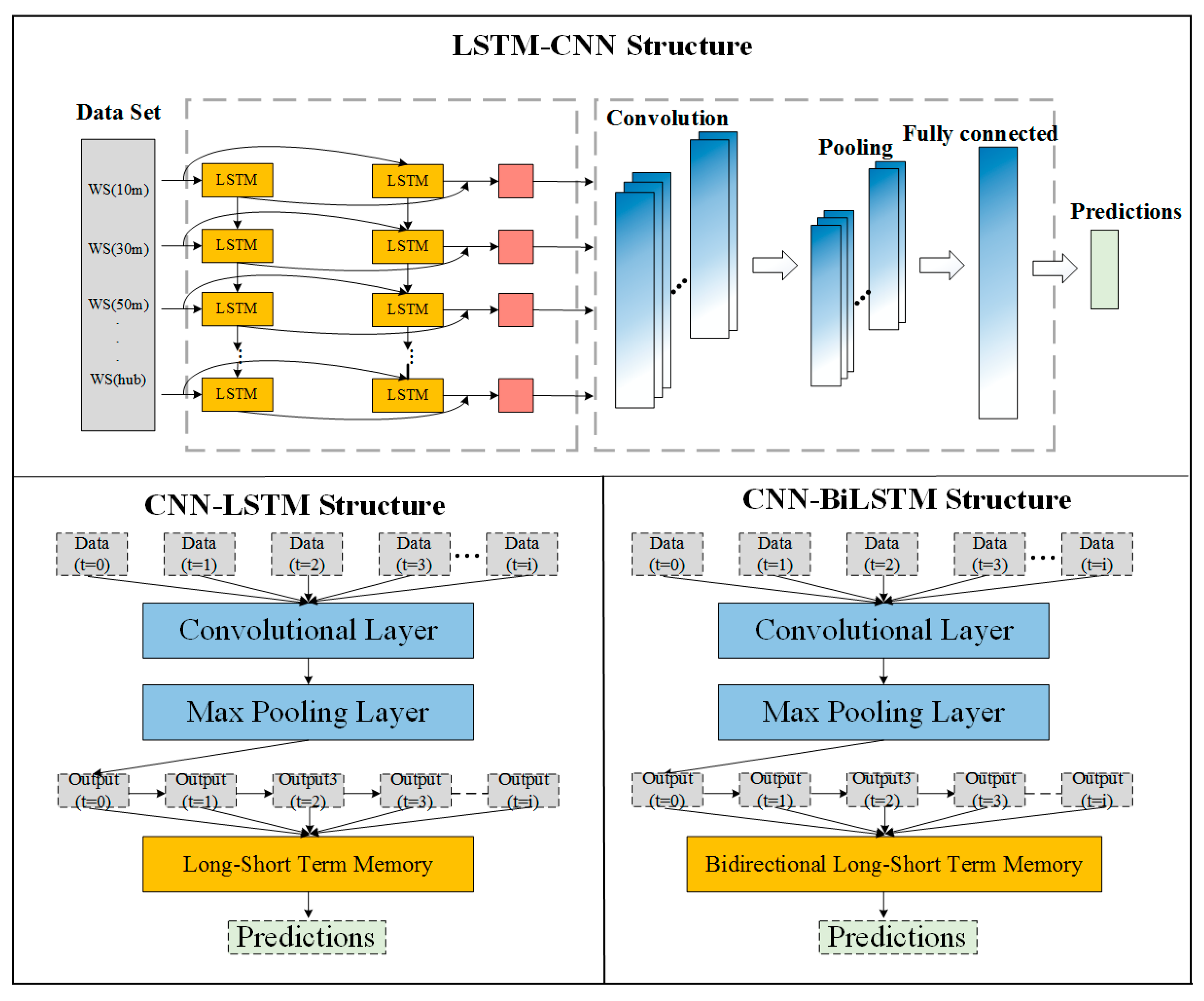
Step3: Validation, comparison and visualization of results. In order to verify the performance of the proposed BiLSTM-CNN model in this paper, three single deep learning models (BiLSTM, LSTM, CNN) and other hybrid deep learning models (LSTM-CNN [17], CNN-BiLSTM [24], CNN-LSTM [16]) are also conducted as comparison models for short-term wind power output prediction. The overall structure of the three hybrid models LSTM-CNN, CNN-LSTM and CNN-BiLSTM are shown in Figure 6. The comparison between different models from various aspects is also conducted. The indicators used to compare model prediction accuracy and efficiency are RMSE, MSE, MAE, R2, Average computational time(s). In order to avoid contingency and increase the reliability of the model, further research chapters are added.

3. Case Study

All experiments were compiled and simulated by the Tensor Flow with Python 3.7 and Intel(R) i7-4850HQ [email protected]. All deep learning based models were. In this section, grey correlation analysis is first utilized to select the input data. Then the parameter settings of proposed BiLSTM-CNN model are described in detail and compared with other deep learning models to verify its effectiveness. Finally, three sets of comparison among deep learning models are conducted to shed lights on the role of CNN and Bi-LSTM as well as the connection mode of model in the short-term wind power forecasting.

3.1. Data Process and Selection

The case study was implemented on a real wind power station. The data set of the wind power station was collected from 15 May 2017 to 31 May 2017, with 4896 samples. The rated installed capacity of the wind power station was 149MW and the temporal resolution of the data set was 5min. The indicators of the original data set include: historical wind power output (WP), wind speed (WS) and wind direction (WD) with different height (30 m, 50 m, 70 m, hub height), relative humidity (H), rainfall (R) and pressure (P). After processing vacancies and outliers on the original data set, the description of the data set is shown in Table 1.
The scientific selection from the original data set can greatly reduce the computing cost and time. Therefore, the selection analysis is a very important process. In this article, we introduce the grey correlational analysis (GCA) to analyze and screen the input based on correlation from the original data set. Different standardization methods may result in different rankings of indicators. Therefore, in this paper, two normalization methods are utilized for the normalization of the data, which is the average value normalization (AVN) and polar difference normalization (PDN). Two normalized methods are described in Formulas (16) and (17). Then, the normalized data are calculated for Grey correlation degree. The results under two different normalization methods are shown in Table 2.
In the average value normalization (AVN) method, each dimension of the data set is normalized to the range of (0–1) by Formula (16):
x ¯ i = x i x min x max x min ,
where x ¯ i is the normalized value, x i is the original data and x max , x min are the maximum and minimum value of the original data respectively.
In polar difference normalization (PDN) method, each dimension of the data set is normalized to the range of (0–1) by Formula (17):
x ¯ i = x i x min x max x min ,
where x ¯ i is the normalized value, x i is the original data and x max , x min are the maximum and minimum value of the original data respectively.
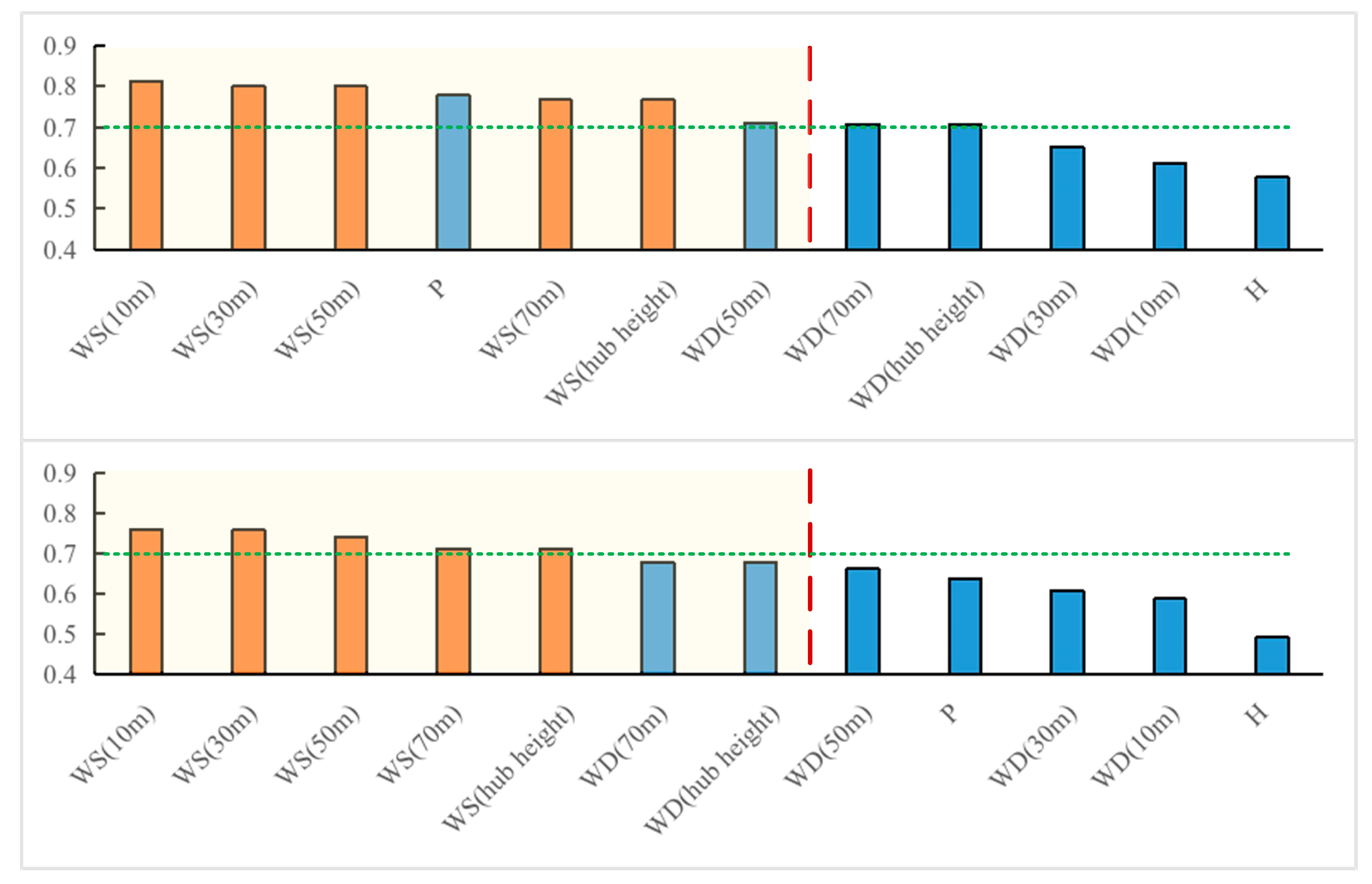
The results of grey correlation analysis under two different normalization methods are intuitively depicted in Figure 7 in descending order. The results show that the two different normalization methods lead to different ranking results. The top three indicators of the two ranking results are the same, namely, wind speed (10 m), wind speed (30 m), wind speed (50 m). And the last three indicators of two ranking results are also the same, namely, wind direction (30 m), wind direction (10 m), humidity.
Five indicators are selected as the input of the forecasting model according to the results from grey correlation analysis, that is, WS (10 m), WS (30 m), WS (50 m), WS (70 m), WS (hub height), which stands for wind speed (10 m), wind speed (30 m), wind speed (50 m), wind speed (70 m) and wind speed (hub height), respectively. The selected five indicators are all relatively high correlated with the target wind power output sequence with grey correlation degrees all bigger than 0.7, which are marked by orange bars in Figure 7.

3.2. Results

3.2.1. Data Set Division and Evaluation Indicators

Data Set is divided into training set, validation set and test set for training optimization and verification of the proposed model, as shown in Figure 8.
To compare the forecasting accuracy of different models, three accuracy evaluation indicators are chosen to evaluate the performance: mean absolute error (MAE), root mean square error (RMSE) and R 2 . These evaluation indicators are calculated as follows:
(1) Root Mean Square Error (RMSE)
e R M S E = 1 N i = 1 N ( x ( i ) x ^ ( i ) ) 2
(2) Mean Absolute Error (MAE)
R 2 = 1 i = 1 N ( x ( i ) x ( i ) ) 2 i = 1 N ( x ( i ) x ¯ ( i ) ) 2
(3) R 2 (R—squared)
R 2 = 1 i = 1 N ( x ( i ) x ( i ) ) 2 i = 1 N ( x ( i ) x ¯ ( i ) ) 2 ,
where x ( i ) is the measured wind power output, x ^ ( i ) is the forecasting wind power value, and N is the size of the evaluation data set. Besides, the average computational time is also calculated to demonstrate the efficiency of each model. Specifically, it refers to the time took for a whole validation attempt of each prediction model.

3.2.2. Experiments and Comparison

In this paper, a hybrid deep learning model based on Bi-LSTM and CNN is developed for short-term wind power output prediction. The specific parameter settings of the model are shown in Table 3. In the proposed model, first, the Bi-LSTM model comprises two hidden layers to learn the bidirectional temporal characteristics of the input historical wind data. The hidden layers have 64 and 128 neurons respectively. Then, two sets of convolution layers and the pooling layer of CNN model are constructed to learn the spatial features among the output of Bi-LSTM. The number of kernels in convolution layers is 64 and 128. Lastly, there is one fully connected layer with 512 neurons to attain the predicted output value of wind power. To prevent the model from over fitting, we also add two dropout layers to model and the dropout rate is 0.2 and 0.1, respectively. Besides, the optimizer is Adam optimizer and the learning rate is 0.001.
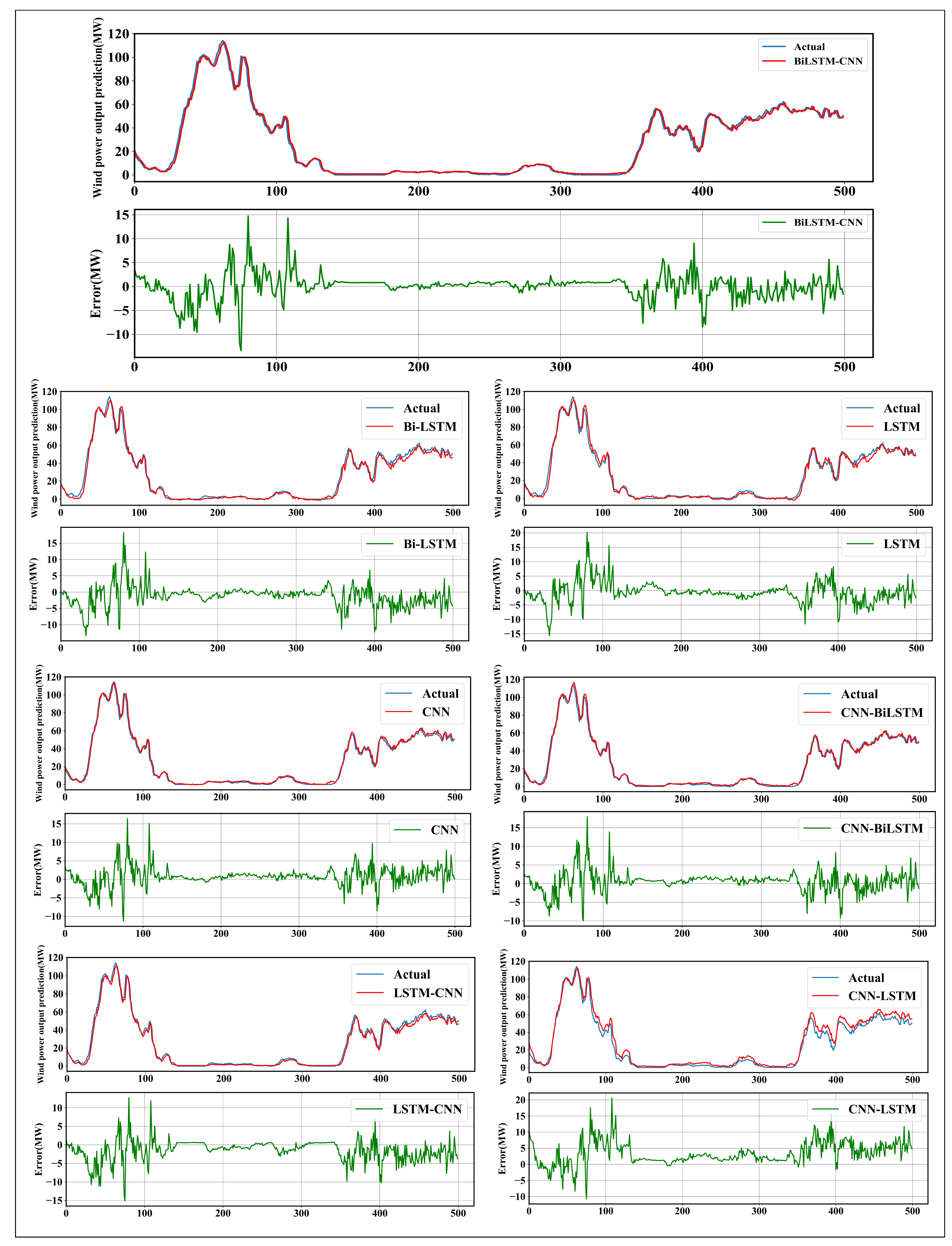
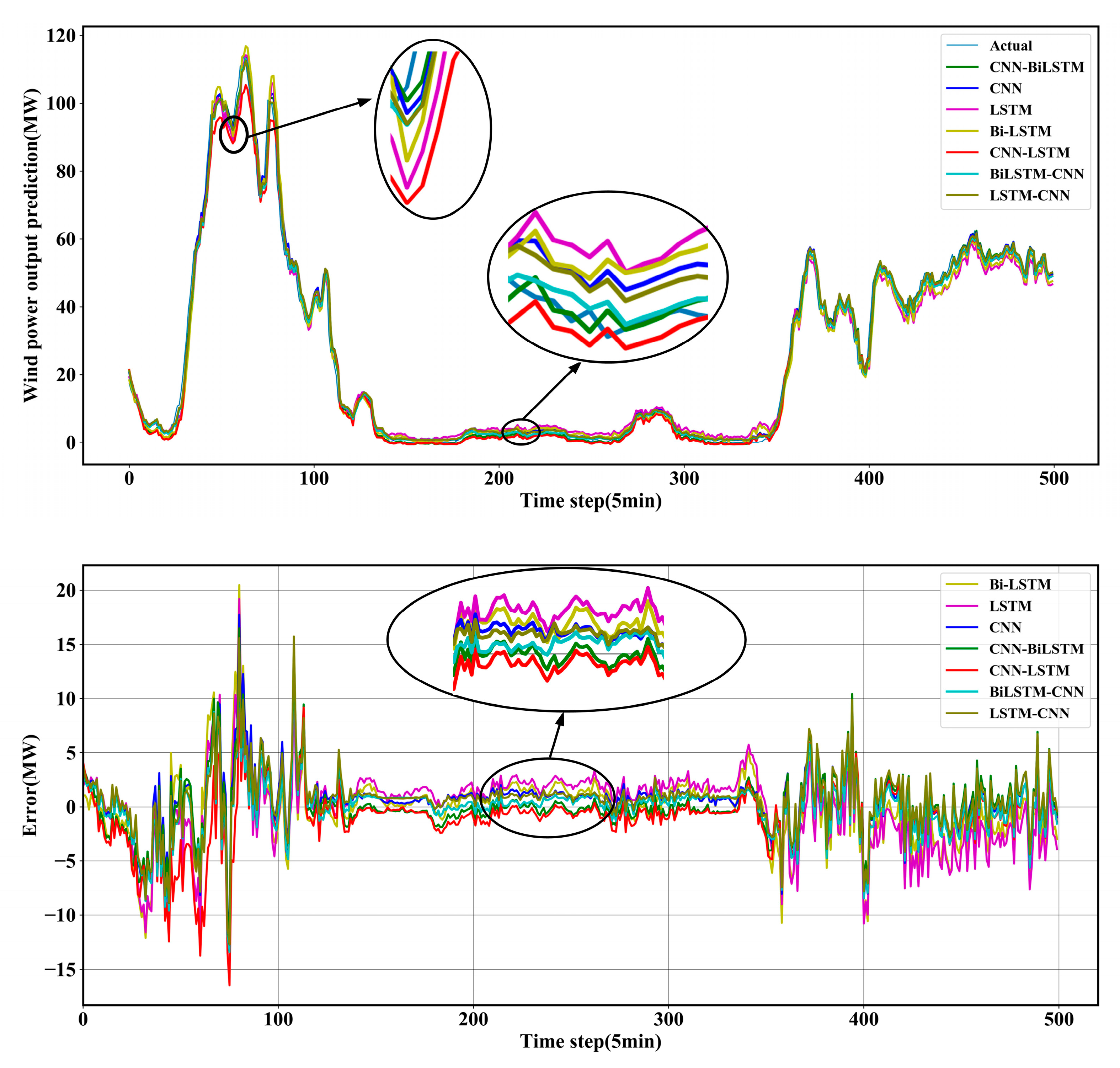
In order to verify the performance of the proposed model, three basic deep learning models (Bi-LSTM, LSTM, CNN) and three combined deep learning models (LSTM-CNN, CNN-BiLSTM, CNN-LSTM) are applied in short-term wind power output prediction as a comparison. All models are based on the same data set. The results of the proposed model and the comparison model are shown in Table 4 and Figure 9. To demonstrate the difference more intuitively among models, the more detailed forecasting results of each model are shown in Figure 10. The prediction result graph and the error comparison graph are separately enlarged shown in Figure 10.
It can be concluded from the results that the proposed hybrid deep learning model BiLSTM-CNN in this paper has the best performance with the lowest RMSE value of 2.5492, MSE value of 6.4984, MAE value of 1.7344 and highest R2 value of 0.9929. From Figure 9 and Figure 10, it can be also seen that the curve of BiLSTM-CNN model is the closest to the real wind power output curve and the prediction error is closer to zero than other models, especially in the time period when wind power changes drastically and rapidly. However, although the prediction accuracy is the highest, the computational speed of BiLSTM-CNN is the slowest with an average computational time of 0.4752 s. In addition, CNN has the fastest calculation speed among all the models with an average computational time of 0.0741 s. And compared with the hybrid model (CNN-BiLSTM, CNN-LSTM, BiLSTM-CNN, LSTM-CNN), all the single models (BiLSTM, LSTM, CNN) have a faster calculation speed with an average computational time 0.2260 s, 0.1274 s, 0.0741 s, respectively.
To further analyze the forecasting results, three sets of comparison is implemented. First, to better analyze the importance of spatial features extracting through the convolution layer and pooling layer of CNN, the 1st set comparison is conducted. Second, to better understand the significance of bidirectional learning characteristic of Bi-LSTM model, the 2nd set comparison is conducted. Finally, we also try to shed lights on the effect of the order of the basic model in the hybrid model, thus the 3rd set comparison is conducted. The three sets of comparison are described in Table 5. And the improved ratio of different model is also introduced in Formula (21) to quantify the difference in the comparison.
I R ( i ) = { ( B ( i ) A ( i ) ) / A ( i ) The   smaller   the   i   indicator ,   the   better ( A ( i ) B ( i ) ) / B ( i ) The   bigger   the   i   indicator ,   the   better
where I R ( i ) refers to the improved ratio of model B on indicator i compared with model A. A ( i ) refers to the performance value of model A on the index i while B ( i ) refers to the performance value of model B on the index i . In this paper, i indicators include RMSE, MSE, MAE, R2, Average computational time. Among them, the smaller the indicators RMSE, MSE, MAE and Average computational time, the better the model prediction performance while R2 is the opposite.
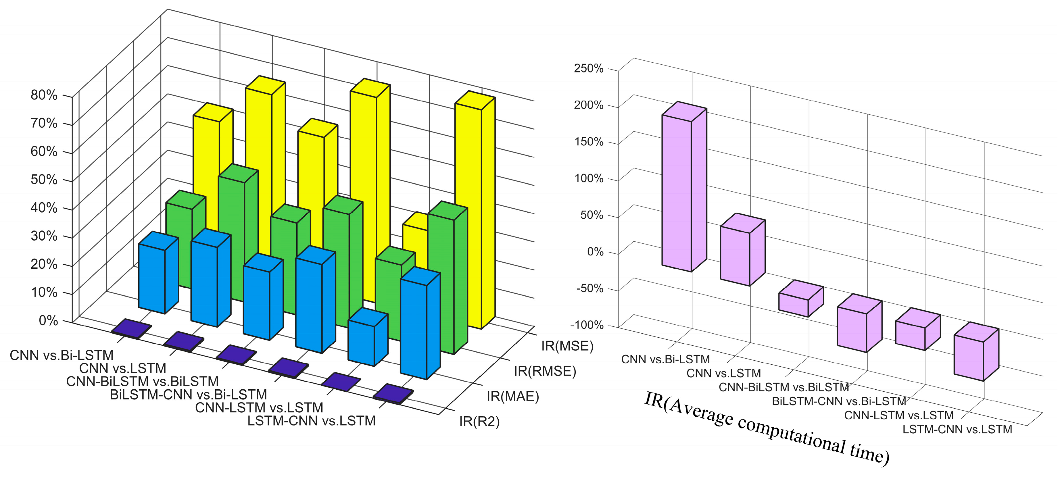
In order to better determine the effectiveness of extracting spatial features through CNN in short-term wind power prediction, we introduced the following model comparison group: CNN vs. Bi-LSTM, CNN vs. LSTM, CNN-BiLSTM vs. BiLSTM, BiLSTM-CNN vs. Bi-LSTM, CNN-LSTM vs. LSTM and LSTM-CNN vs. LSTM. The comparison results are shown in Table 6 and Figure 11. Among the three single models, CNN has the best performance and the fastest running speed with the lowest RMSE of 2.7343, MSE of 7.4766, MAE of 1.8983, average computational time of 0.0741 and the highest R2 0.9918. Compared with Bi-LSTM and LSTM, CNN has higher prediction accuracy and faster average operation speed, with IR (RMSE), IR (MSE), IR(MAE), IR(R2) and IR(Average computational time) all positive value.
Compared with the single model Bi-LSTM, the improved ratio of RMSE, MSE, MAE, R2, average computational time of CNN-BiLSTM are 24.13%, 54.09%, 32.64%, 0.44%, and−23.19%, respectively. Compared with the single model Bi-LSTM, the improved ratio of RMSE, MSE, MAE, R2, average computational time of BiLSTM-CNN are 31.50%, 72.92%, 40.32%, 0.53% and −52.44%, respectively. Compared with the single model LSTM, the improved ratio of RMSE, MSE, MAE, R2, average computational time of CNN-LSTM are 14.13%, 30.25%, 27.02%, −1.04%, −30.66%, respectively. Compared with the single model LSTM, the improved ratio of RMSE, MSE, MAE, R2, average computational time of LSTM-CNN are 33.35%, 77.81%, 47.59%, 0.60%, −53.12%, respectively. We can conclude that the CNN-BiLSTM and BiLSTM-CNN model all have a higher accuracy and lower running speed than single Bi-LSTM model and the CNN-LSTM and BiLSTM-CNN model has a higher accuracy and lower running speed than single LSTM model. It can be summarized that the ability of CNN to extract spatial features from multiple wind speed series at different height model is of great significance in improving the accuracy of short-term wind output prediction but hybrid models with CNN often need more computational time to mine the complex relationship between the input sequences and wind power output.
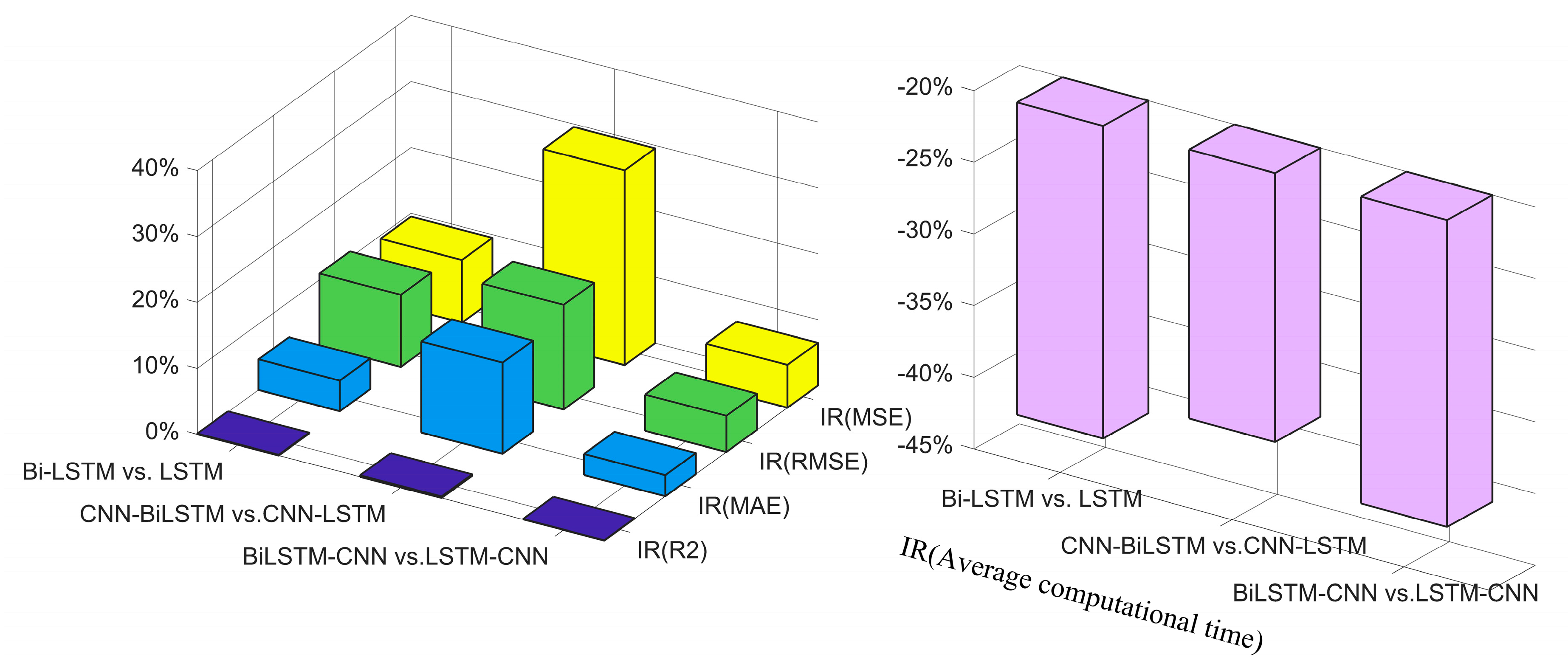
In order to better determine the effectiveness of extracting temporal features through Bi-LSTM in short-term wind power prediction, we introduced the following model comparison group: Bi-LSTM vs. LSTM, CNN-BiLSTM vs. CNN-LSTM, BiLSTM-CNN vs. LSTM-CNN. The comparison results are shown in Table 7 and Figure 12.
Compared with the model LSTM, the improved ratio of RMSE, MSE, MAE, R2, average computational time of BiLSTM are 4.65%, 9.51%, 10.95%, 0.12% and −43.61%, respectively. Compared with the model CNN-LSTM, the improved ratio of RMSE, MSE, MAE, R2, average computational time of CNN-BiLSTM are 13.82%, 29.55%, 15.87%, 0.24% and −37.53%, respectively. Compared with the model LSTM-CNN, the improved ratio of RMSE, MSE, MAE, R2, average computational time of BiLSTM-CNN are 3.20%, 6.49%, 5.49%, 0.05%, −42.80%, respectively. It can be concluded that compared with LSTM, the Bi-LSTM model or the hybrid model containing Bi-LSTM has higher prediction accuracy in short-term wind power output prediction, because the bidirectional learning characteristic of Bi-LSTM can better mine the temporal feature between the multiple input time series data and historical wind power output time series. However, compared with LSTM, Bi-LSTM model or hybrid model has more parameters in the forecasting process, which results in the relatively low computational speed.
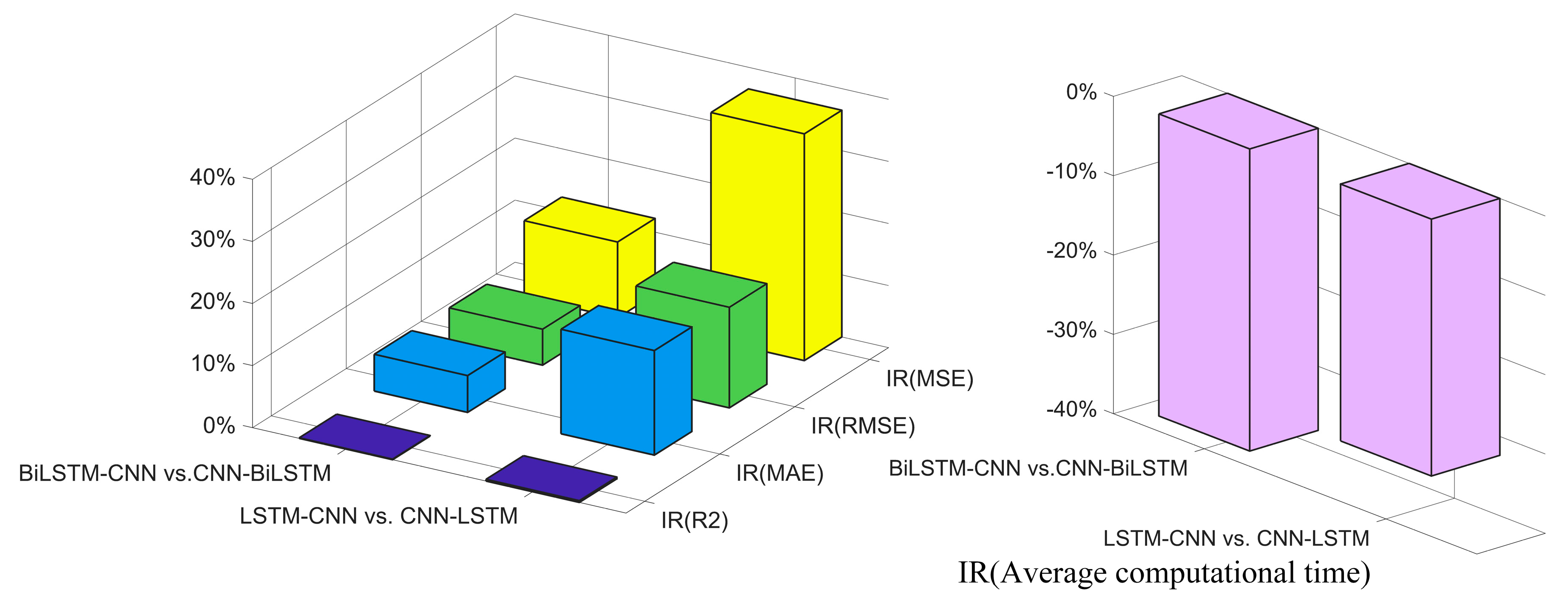
Finally, we conduct two groups of comparison among hybrid models: BiLSTM-CNN vs. CNN-BiLSTM and LSTM-CNN vs. CNN-LSTM. By applying different deep learning model, the order to extract spatial and temporal features may be different. Therefore, the goal of this comparison is to determine influence of the sequence order of single model (CNN, LSTM, Bi-LSTM) in hybrid model on the prediction. The comparison results are shown in Table 8 and Figure 13.
Compared with the model CNN-BiLSTM, the improved ratio of RMSE, MSE, MAE, R2, average computational time of BiLSTM-CNN are 5.93%, 12.22%, 5.79%, 0.09% and −38.08%, respectively. Compared with the model CNN-LSTM, the improved ratio of RMSE, MSE, MAE, R2, average computational time of LSTM-CNN are 16.84%, 36.52%, 16.20%, 0.28% and −32.38%, respectively. From the results of the comparison, it can be concluded that BiLSTM-CNN has a higher prediction accuracy and a lower computational speed than CNN-BiLSTM; LSTM-CNN has a higher prediction accuracy and a lower computational speed than CNN-LSTM. To attain a higher prediction accuracy, it is better to ‘extracting the temporal characteristics of the input historical sequences first and extracting the spatial characteristics second’ than ‘extracting the spatial features among the input historical sequences first and then extracting the temporal features’.

3.2.3. Further Study

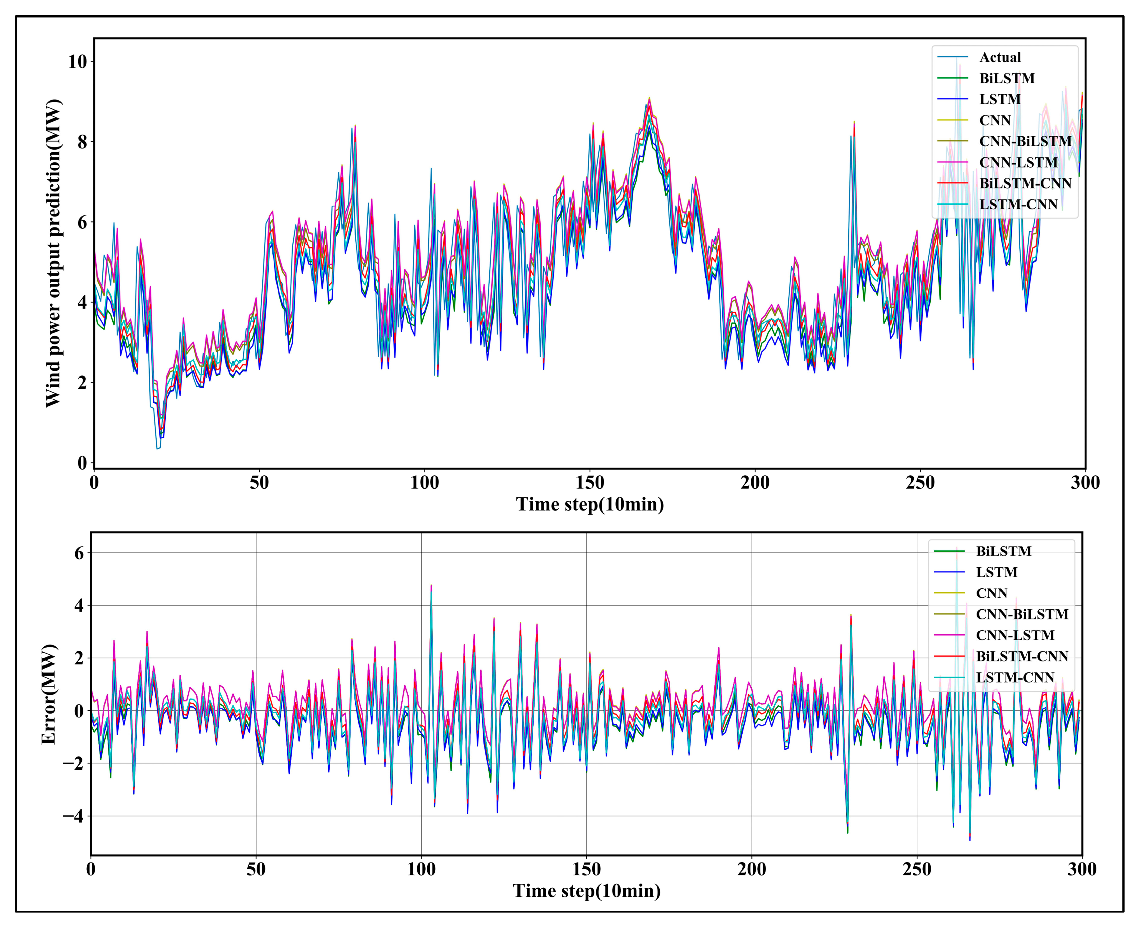
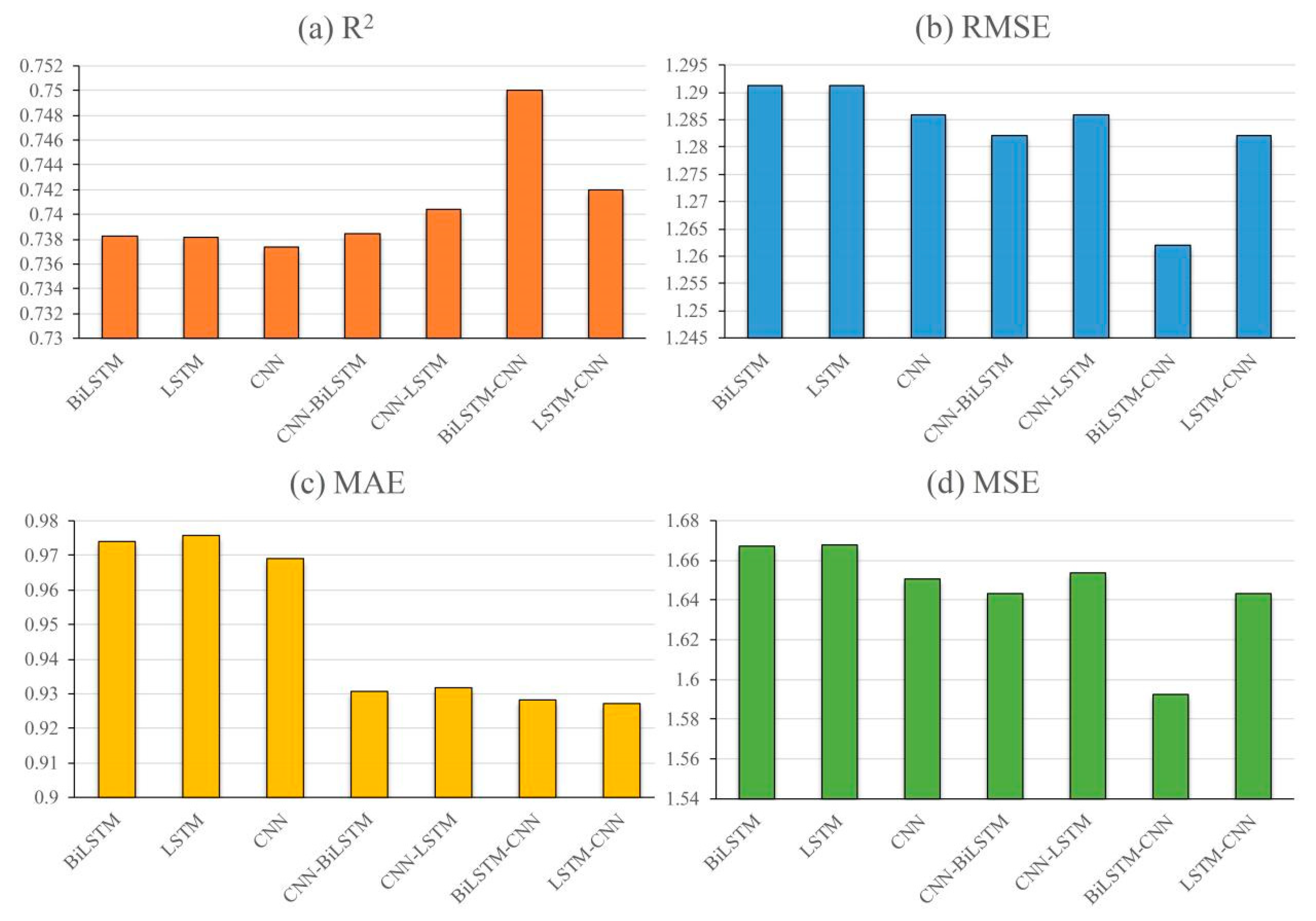
In order to further validate the adaptability and robustness of the proposed BiLSTM-CNN model, another case study with data set acquired from a wind farm in Shanxi province in China is experimented and conducted, the data of which spans from 1 January 2019 to 31 December 2019 (50954 samples). The resolution of this data set is 10 min. The whole data set is divided into the training set, validation set and test set for training optimization and verification, which account for 60%, 25% and 15% respectively. The proposed forecasting model BiLSTM-CNN along with other comparative models(LSTM, CNN, CNN-LSTM, CNN-BiLSTM, LSTM-CNN) are trained with this data set to forecast the short-term wind power. The forecasting results and error results are demonstrated in Figure 14. The evaluation criteria results of the different model are shown in Figure 15.
As shown in Figure 14 and Figure 15, the forecasting curve of the proposed model is the closest to the actual wind power output curve with the lowest MAE, RMSE, MAPE and highest R2. BiLSTM-CNN model has a better performance considering the forecasting accuracy than other comparative models (LSTM, CNN, CNN-LSTM, CNN-BiLSTM, LSTM-CNN). Therefore, the proposed BiLSTM-CNN can handle the short term wind power prediction with high accuracy, which is consistent with the results of the case study in Section 3.2.2. Besides, From the evaluation results, it can be concluded that in this case of further study, BiLSTM-CNN still has a higher prediction accuracy than CNN-BiLSTM and LSTM-CNN has a higher prediction accuracy performance than CNN-LSTM, which verifies the statement that ‘extracting the temporal feature first and later extracting the spatial feature’ is better than ‘extracting the spatial feature first and later extracting the temporal feature’ according to the short term wind power forecasting problem.

4. Conclusions and Discussion

In this paper, to better predict the short-term wind power output, grey correlation analysis is applied to select highly correlated indicators at first. Then a hybrid short-term wind power forecasting model based on bidirectional long short time memory neural network and convolutional neural networks, which is BiLSTM-CNN network model, is proposed. The proposed model takes into account the distinct temporal and spatial features of input data for short-term wind power forecasting. Finally, various single deep learning (Bi-LSTM, LSTM, CNN) and their combined model (LSTM-CNN, CNN-BiLSTM, CNN-LSTM) are also applied and simulated to verify the performance of the proposed model. Also, the comparison among these models from three main facets is also conducted to catch a sight of hint about how to improve forecasting method through model combination to extract compound characteristic. The main conclusion is listed below:
First, the input indicators of the wind power forecasting model are screened and analyzed through grey correlation analysis under two different normalization methods. Multiple wind speed time series data with different heights are selected as inputs of the proposed model and comparison model with the highest and steadiest grey correlation degree.
Second, the BiLSTM-CNN model is innovatively proposed and applied in the application of wind power forecasting with the lowest RMSE value of 2.5492, MSE value of 6.4984, MAE value of 1.7344, the highest R2 value of 0.9929. The hybrid model mainly predicts the short-term wind power output by taking advantage of the temporal-spatial features extraction ability of the proposed model to construct the complex relationship between the input data and target wind power output, where the Bi-LSTM model is utilized to mine the temporal characteristics of the input time series data and the convolution and pooling operations of CNN model is utilized to extract the spatial characteristics of multiple input time series data.
Third, three sets of comparison among different deep learning models are systematically studied from various aspects in wind power forecasting. The role of CNN to extract spatial features through the convolution layer and pooling layer and Bi-LSTM to grasp temporal features can significantly improve the predication accuracy. Besides, the mode that extracts the temporal feature first and then extracts the spatial feature is better than the mode extract the spatial feature first and then extract the temporal feature, which is verified in both the case study and further study.
In short, this paper starts with characteristics of wind power input data, then proposed a hybrid deep learning model BiLSTM-CNN to predict the short-term wind power and compares the performance of seven deep learning models in wind power prediction. In the following research, the hybrid model with other advanced deep learning models can be better optimized to extract the temporal-spatial features separately in order to obtain more accurate wind power prediction results. There is also room for improvement in the speed of the hybrid model.

Author Contributions

Conceptualization, H.Z.; Data curation, H.Z. and M.Y.; Funding acquisition, X.X.; Investigation, H.Z. and M.Y.; Methodology, H.Z. and K.W.; Project administration, D.N. and Y.L.; Resources, Y.L. and X.X.; Software, H.Z.; Supervision, Y.L. and D.N.; Validation, H.Z., M.Y. and K.W.; Writing—original draft, H.Z., M.Y. and K.W.; Writing—review & editing, K.W. and H.Z. All authors have read and agreed to the published version of the manuscript.

Funding

This work is supported by the 2018 Key Projects of Philosophy and Social Sciences Research, Ministry of Education, China (Project No. 18JZD032), 111 Project, Ministry of Science and Technology of People’s Republic of China (Project No. B18021), Natural Science Foundation of China (Project No. 71804045), Natural Science Foundation of Hebei Province, China (Project No. G2020403008) and Humanities and Social Science Research Project of Hebei Education Department, China (Project No. SQ201097).

Conflicts of Interest

The authors declare no conflict of interest.

References

  1. Aly, H.H. A Novel Deep Learning Intelligent Clustered Hybrid Models for Wind Speed and Power Forecasting. Energy 2020, 213, 118773. [Google Scholar] [CrossRef]
  2. Afshar, K.; Ghiasvand, F.S.; Bigdeli, N. Optimal bidding strategy of wind power producers in pay-as-bid power markets. Renew. Energy 2018, 127, 575–586. [Google Scholar] [CrossRef]
  3. Global Wind Report 2019|Global Wind Energy Council. Available online: https://gwec.net/global-wind-report-2019/ (accessed on 10 October 2020).
  4. Naik, J.; Bisoi, R.; Dash, P. Prediction interval forecasting of wind speed and wind power using modes decomposition based low rank multi-kernel ridge regression. Renew. Energy 2018, 129, 357–383. [Google Scholar] [CrossRef]
  5. Wang, K.; Niu, D.; Sun, L.; Zhen, H.; Liu, J.; De, G.; Xu, X. Wind Power Short-Term Forecasting Hybrid Model Based on CEEMD-SE Method. Processes 2019, 7, 843. [Google Scholar] [CrossRef] [Green Version]
  6. Lahouar, A.; Slama, J.B.H. Hour-ahead wind power forecast based on random forests. Renew. Energy 2017, 109, 529–541. [Google Scholar] [CrossRef]
  7. James, E.P.; Benjamin, S.G.; Marquis, M. Offshore wind speed estimates from a high-resolution rapidly updating numerical weather prediction model forecast dataset. Wind Energy 2018, 21, 264–284. [Google Scholar] [CrossRef]
  8. Zuluaga, C.D.; Alvarez, M.A.; Giraldo, E. Short-term wind speed prediction based on robust Kalman filtering: An experimental comparison. Appl. Energy 2015, 156, 321–330. [Google Scholar] [CrossRef]
  9. Torres, J.L.; Garcia, A.; De Blas, M.; De Francisco, A. Forecast of hourly average wind speed with ARMA models in Navarre (Spain). Sol. Energy 2005, 79, 65–77. [Google Scholar] [CrossRef]
  10. Sfetsos, A. A novel approach for the forecasting of mean hourly wind speed time series. Renew. Energy 2002, 27, 163–174. [Google Scholar] [CrossRef]
  11. Cadenas, E.; Jaramillo, O.A.; Rivera, W. Analysis and forecasting of wind velocity in chetumal, quintana roo, using the single exponential smoothing method. Renew. Energy 2010, 35, 925–930. [Google Scholar] [CrossRef]
  12. Samet, H.; Marzbani, F. Quantizing the deterministic nonlinearity in wind speed time series. Renew. Sustain. Energy Rev. 2014, 39, 1143–1154. [Google Scholar] [CrossRef]
  13. Ouyang, T.; Zha, X.; Qin, L. A combined multivariate model for wind power prediction. Energy Convers. Manag. 2017, 144, 361–373. [Google Scholar] [CrossRef]
  14. Marugán, A.P.; Márquez, F.P.G.; Perez, J.M.P.; Ruiz-Hernández, D. A survey of artificial neural network in wind energy systems. Appl. Energy 2018, 228, 1822–1836. [Google Scholar] [CrossRef] [Green Version]
  15. Barman, M.; Choudhury, N.B.D. Season specific approach for short-term load forecasting based on hybrid FA-SVM and similarity concept. Energy 2019, 174, 886–896. [Google Scholar] [CrossRef]
  16. Tso, G.K.; Yau, K.K. Predicting electricity energy consumption: A comparison of regression analysis, decision tree and neural networks. Energy 2007, 32, 1761–1768. [Google Scholar] [CrossRef]
  17. Voyant, C.; Notton, G.; Kalogirou, S.; Nivet, M.-L.; Paoli, C.; Motte, F.; Fouilloy, A. Machine learning methods for solar radiation forecasting: A review. Renew. Energy 2017, 105, 569–582. [Google Scholar] [CrossRef]
  18. Li, L.-L.; Zhao, X.; Tseng, M.-L.; Tan, R.R. Short-term wind power forecasting based on support vector machine with improved dragonfly algorithm. J. Clean. Prod. 2020, 242, 118447. [Google Scholar] [CrossRef]
  19. Liu, M.; Cao, Z.; Zhang, J.; Wang, L.; Huang, C.; Luo, X. Short-term wind speed forecasting based on the Jaya-SVM model. Int. J. Electr. Power Energy Syst. 2020, 121, 106056. [Google Scholar] [CrossRef]
  20. Wang, G.; Jia, R.; Liu, J.; Zhang, H. A hybrid wind power forecasting approach based on Bayesian model averaging and ensemble learning. Renew. Energy 2020, 145, 2426–2434. [Google Scholar] [CrossRef]
  21. Rodríguez, F.; Florez-Tapia, A.M.; Fontán, L.; Galarza, A. Very short-term wind power density forecasting through artificial neural networks for microgrid control. Renew. Energy 2020, 145, 1517–1527. [Google Scholar] [CrossRef]
  22. Hinton, G.E.; Osindero, S.; Teh, Y.-W. A fast learning algorithm for deep belief nets. Neural Comput. 2006, 18, 1527–1554. [Google Scholar] [CrossRef] [PubMed]
  23. LeCun, Y.; Bottou, L.; Bengio, Y.; Haffner, P. Gradient-based learning applied to document recognition. Proc. IEEE 1998, 86, 2278–2324. [Google Scholar] [CrossRef] [Green Version]
  24. Hochreiter, S.; Schmidhuber, J. Long short-term memory. Neural Comput. 1997, 9, 1735–1780. [Google Scholar] [CrossRef] [PubMed]
  25. Goodfellow, I.; Pouget-Abadie, J.; Mirza, M.; Xu, B.; Warde-Farley, D.; Ozair, S.; Courville, A.; Bengio, Y. Generative Adversarial Networks. arXiv 2014, arXiv:1406.2661. [Google Scholar]
  26. He, K.; Zhang, X.; Ren, S.; Sun, J. Deep residual learning for image recognition. arXiv 2016, arXiv:1512.03385. [Google Scholar]
  27. Wang, K.; Qi, X.; Liu, H. Photovoltaic power forecasting based LSTM-Convolutional Network. Energy 2019, 189, 116225. [Google Scholar] [CrossRef]
  28. He, W. Load forecasting via deep neural networks. Procedia Comput. Sci. 2017, 122, 308–314. [Google Scholar] [CrossRef]
  29. Díaz–Vico, D.; Torres–Barrán, A.; Omari, A.; Dorronsoro, J.R. Deep neural networks for wind and solar energy prediction. Neural Process. Lett. 2017, 46, 829–844. [Google Scholar] [CrossRef]
  30. Hong, Y.-Y.; Rioflorido, C.L.P.P. A hybrid deep learning-based neural network for 24-h ahead wind power forecasting. Appl. Energy 2019, 250, 530–539. [Google Scholar] [CrossRef]
  31. Qing, X.; Niu, Y. Hourly day-ahead solar irradiance prediction using weather forecasts by LSTM. Energy 2018, 148, 461–468. [Google Scholar] [CrossRef]
  32. Gao, M.; Li, J.; Hong, F.; Long, D. Day-ahead power forecasting in a large-scale photovoltaic plant based on weather classification using LSTM. Energy 2019, 187, 115838. [Google Scholar] [CrossRef]
  33. Cai, M.; Pipattanasomporn, M.; Rahman, S. Day-ahead building-level load forecasts using deep learning vs. traditional time-series techniques. Appl. Energy 2019, 236, 1078–1088. [Google Scholar] [CrossRef]
  34. Duan, M.; Li, K.; Yang, C.; Li, K. A hybrid deep learning CNN–ELM for age and gender classification. Neurocomputing 2018, 275, 448–461. [Google Scholar] [CrossRef]
  35. Wang, H.; Yang, Z.; Yu, Q.; Hong, T.; Lin, X. Online reliability time series prediction via convolutional neural network and long short term memory for service-oriented systems. Knowl.-Based Syst. 2018, 159, 132–147. [Google Scholar] [CrossRef]
  36. Bao, J.; Liu, P.; Ukkusuri, S.V. A spatiotemporal deep learning approach for citywide short-term crash risk prediction with multi-source data. Accid. Anal. Prev. 2019, 122, 239–254. [Google Scholar] [CrossRef] [PubMed]
  37. Wen, C.; Liu, S.; Yao, X.; Peng, L.; Li, X.; Hu, Y.; Chi, T. A novel spatiotemporal convolutional long short-term neural network for air pollution prediction. Sci. Total Environ. 2019, 654, 1091–1099. [Google Scholar] [CrossRef] [PubMed]
  38. Liu, H.; Mi, X.; Li, Y. Smart deep learning based wind speed prediction model using wavelet packet decomposition, convolutional neural network and convolutional long short term memory network. Energy Convers. Manag. 2018, 166, 120–131. [Google Scholar] [CrossRef]
  39. Wang, J.-Z.; Wang, Y.; Jiang, P. The study and application of a novel hybrid forecasting model–A case study of wind speed forecasting in China. Appl. Energy 2015, 143, 472–488. [Google Scholar] [CrossRef]
  40. Jiang, P.; Wang, Y.; Wang, J. Short-term wind speed forecasting using a hybrid model. Energy 2017, 119, 561–577. [Google Scholar] [CrossRef]
  41. Gu, J.; Wang, Z.; Kuen, J.; Ma, L.; Shahroudy, A.; Shuai, B.; Liu, T.; Wang, X.; Wang, G.; Cai, J. Recent advances in convolutional neural networks. Pattern Recognit. 2018, 77, 354–377. [Google Scholar] [CrossRef] [Green Version]
  42. Huang, Y.; Shen, L.; Liu, H. Grey relational analysis, principal component analysis and forecasting of carbon emissions based on long short-term memory in China. J. Clean. Prod. 2019, 209, 415–423. [Google Scholar] [CrossRef]
  43. Atef, S.; Eltawil, A.B. Assessment of stacked unidirectional and bidirectional long short-term memory networks for electricity load forecasting. Electr. Power Syst. Res. 2020, 187, 106489. [Google Scholar] [CrossRef]
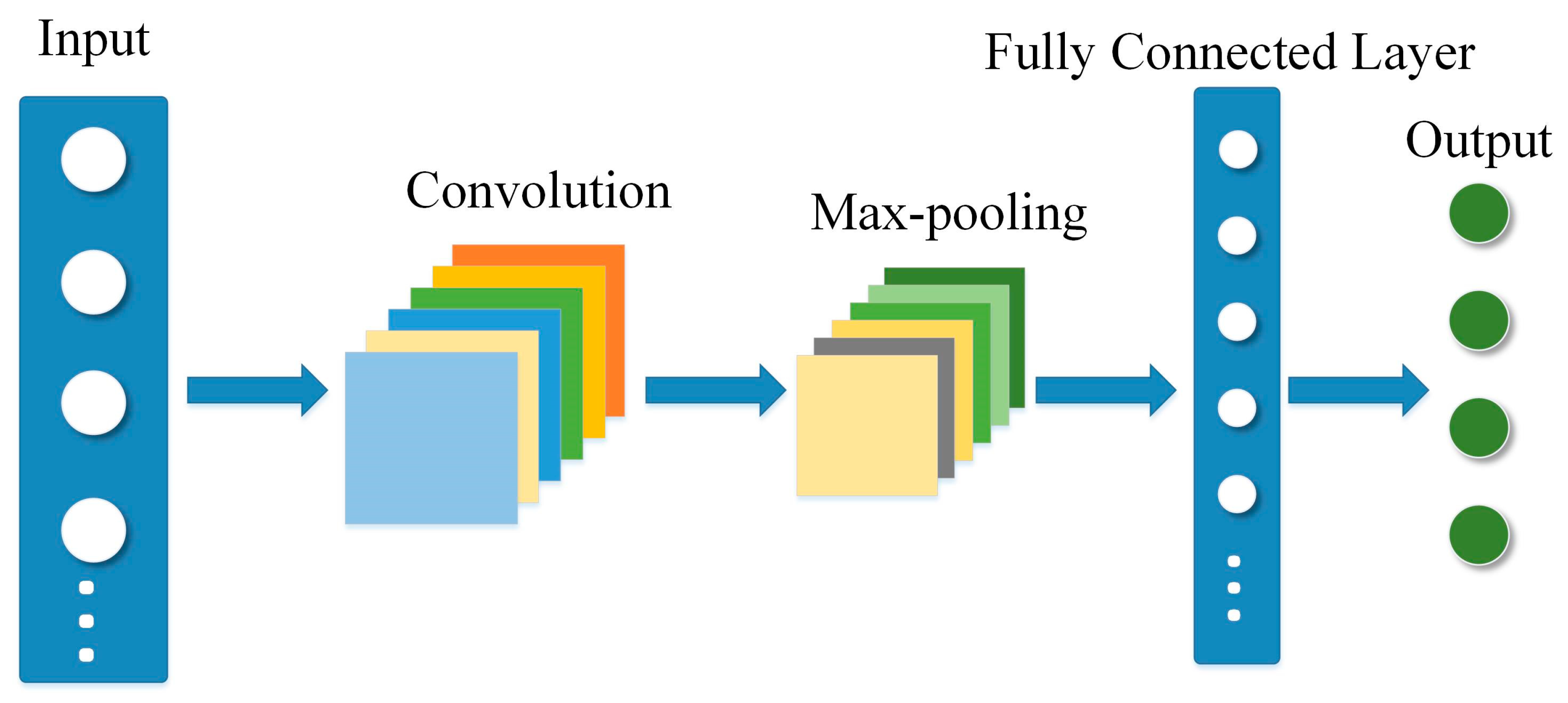
Figure 1. Convolutional Neural Network (CNN) structure.
Sustainability 12 09490 g001
Figure 2. Internal structure of LSTM.
Sustainability 12 09490 g002
Figure 3. Network structure of Bi-LSTM [43].
Sustainability 12 09490 g003
Figure 4. Proposed hybrid deep learning BiLSTM-CNN model structure.
Sustainability 12 09490 g004
Figure 5. Framework of proposed model.
Sustainability 12 09490 g005
Figure 6. The structure of hybrid models LSTM-CNN, CNN-LSTM and CNN-BiLSTM.
Sustainability 12 09490 g006
Figure 7. Input data selection through grey correlation analysis.
Sustainability 12 09490 g007
Figure 8. Data Set division.
Sustainability 12 09490 g008
Figure 9. Results of different models for wind power forecasting.
Sustainability 12 09490 g009
Figure 10. Results comparison of different models for wind power forecasting.
Sustainability 12 09490 g010
Figure 11. Results of 1st set of comparison.
Sustainability 12 09490 g011
Figure 12. Results of 2nd set of comparison.
Sustainability 12 09490 g012
Figure 13. Results of 3rd set of comparison.
Sustainability 12 09490 g013
Figure 14. Forecasting results of proposed model and other comparative models.
Sustainability 12 09490 g014
Figure 15. Evaluation criteria results of forecasting models.
Sustainability 12 09490 g015
Table 1. Detailed description of the data set.
WPWS (10 m)WD (10 m)WS (30 m)WD (30 m)WS (50 m)WD (50 m)
Count4597459745974597459745974597
Mean38.914.55118.795.20120.605.45120.62
Std33.812.3599.142.69101.102.80100.66
Min00.1300.1700.130
Max143.0915.8636019.1536019.64360
WS (70 m)WD (70 m)WS (hub height)WD (hub height)Pressure (P)Humidity (H)
Count459745974597459745974597
Mean5.62123.325.62123.32952.9852.251817
Std2.8699.902.8699.905.1824.32
Min0.1500.150941.344.01
Max20.7536020.75360963.0499.027
Table 2. Results of grey correlation analysis.
Standard MethodGrey Correlation Degree and Ranking Sequences
WS
(10 m)
WD
(10 m)
WS
(30 m)
WD
(30 m)
WS
(50 m)
WD
(50 m)
WS
(70 m)
WD
(70 m)
WS
(Hub Height)
WD
(Hub Height)
PH
PDN0.811 0.610 0.800 0.652 0.800 0.710 0.767 0.708 0.767 0.708 0.778 0.577
Ranking: WS (10 m) > WS (30 m) > WS (50 m) > P > WS (70 m) > WS (hub height) > WD (50 m) > WD (70 m) > WD (hub height) > WD (30 m) > WD (10 m) > H
AVN0.761 0.587 0.758 0.608 0.742 0.662 0.712 0.677 0.712 0.677 0.636 0.492
Ranking: WS (10 m) > WS (30 m) > WS (50 m) > WS (70 m) > WS (hub height) > WD (70 m) > WD (hub height) > WD (50 m) > P > WD (30 m) > WD (10 m) > H
Table 3. Parameter settings of the proposed models.
Proposed ModelConfiguration
BiLSTM-CNNBi-LSTMUnits1Units = 64;Epoch = 80,
Batch size = 100; Optimizer = ‘Adam’; Learning rate = 0.001.
Units2Units = 128;
Drop outDrop out = 0.2
CNNConvolutionFilter = 64; Kernel size = 3; Stride = 1
Max-poolingKernel size = 2; Stride = 1
ConvolutionFilter = 128; Kernel size = 3; Stride = 1
Max-poolingKernel size = 2; Stride = 1
Drop outDrop out = 0.1
Fully connectedNeurons = 512
Table 4. Result of the proposed model.
Single ModelHybrid Model
Bi-LSTMLSTMCNNCNN-BiLSTMCNN-LSTMBiLSTM-CNNLSTM-CNN
RMSE:3.3522 3.5079 2.7343 2.7005 3.0737 2.5492 2.6307
MSE:11.2369 12.3053 7.4766 7.2926 9.4475 6.4984 6.9204
MAE:2.4338 2.7004 1.8983 1.8349 2.1261 1.7344 1.8296
R2:0.9877 0.9865 0.9918 0.9920 0.9896 0.9929 0.9924
Average computational time(s):0.2260 0.1274 0.0741 0.2942 0.1838 0.4752 0.2718
Table 5. Model comparison.
Description
1st set
comparison
CNN vs. Bi-LSTM; CNN vs. LSTM;
CNN-BiLSTM vs. BiLSTM; BiLSTM-CNN vs. Bi-LSTM;
CNN-LSTM vs.LSTM; LSTM-CNN vs. LSTM
2nd set
comparison
Bi-LSTM vs. LSTM;
CNN-BiLSTM vs. CNN-LSTM; BiLSTM-CNN vs. LSTM-CNN
3rd set comparisonBiLSTM-CNN vs. CNN-BiLSTM; LSTM-CNN vs. CNN-LSTM
Table 6. 1st set of comparison.
CNN vs. Bi-LSTMCNN vs. LSTMCNN-BiLSTM vs. BiLSTMBiLSTM-CNN vs. Bi-LSTMCNN-LSTM vs. LSTMLSTM-CNN vs. LSTM
IR(RMSE)22.59%28.29%24.13%31.50%14.13%33.35%
IR(MSE)50.29%64.58%54.09%72.92%30.25%77.81%
IR(MAE)28.21%42.26%32.64%40.32%27.02%47.59%
IR(R2)0.42%0.54%0.44%0.53%−1.04%0.60%
IR(Average computational time)204.90%71.92%−23.19%−52.44%−30.66%−53.12%
Table 7. 2nd set comparison.
Bi-LSTM vs. LSTMCNN-BiLSTM vs. CNN-LSTMBiLSTM-CNN vs. LSTM-CNN
IR(RMSE)4.65%13.82%3.20%
IR(MSE)9.51%29.55%6.49%
IR(MAE)10.95%15.87%5.49%
IR(R2)0.12%0.24%0.05%
IR(Average computational time)−43.61%−37.53%−42.80%
Table 8. 3rd set comparison.
BiLSTM-CNN vs. CNN-BiLSTMLSTM-CNN vs. CNN-LSTM
IR(RMSE)5.93%16.84%
IR(MSE)12.22%36.52%
IR(MAE)5.79%16.20%
IR(R2)0.09%0.28%
IR(Average computational time)−38.08%−32.38%
Publisher’s Note: MDPI stays neutral with regard to jurisdictional claims in published maps and institutional affiliations.