On the Effectiveness of the Measures in Supermarkets for Reducing Contact among Customers during COVID-19 Period

Abstract

The spread of the COVID-19 virus had a huge impact on human life on the global scale. Many control measures devoted to decrease contact among people have been adopted to slow down the transmission of the disease. A series of measures have been taken in supermarkets, which include restricting the number of customers, keeping social distance, and entering with a shopping cart. In this work, we investigate with numerical simulations the effectiveness of these measures in reducing the contact among customers. Several scenarios with different control measures are designed for numerical analysis. The movements of customers in a supermarket are simulated by a microscopic model for pedestrian dynamics. Moreover, an index based on the distance between customers is defined to measure the degree of contact and therefore evaluate it quantitatively. The effect of these measures on the average contact degree of each customer is explored, and the spatial distribution of the contact among customers in the supermarket is shown in a qualitative way. Simulation results show that except shopping cart measure, the other two measures are effective in reducing contact among customers.

1. Introduction

The so-called Coronavirus (COVID-19) was first identified in December 2019 in Wuhan, Hubei, China and has became an infectious disease worldwide [1]. As of 29 June 2020, there have been more than 10 million confirmed cases of COVID-19, including nearly 500,000 deaths, as reported by the World Health Organization (WHO) [2]. The disease spreads primarily from person to person through small droplets produced by coughing, sneezing, or speaking of an infected person [3]. Therefore, as there is still no known vaccine against the virus, reducing close contact situations among people is one of the recommended measures to prevent infection [4]. Other measures taken by many countries to avoid or even prohibit situations leading to close contact among people, including travel restrictions, closing schools, and canceling large gatherings. The effectiveness of these control measures are investigated in some works [5,6,7].

The pandemic and these control measures also have a huge impact on pedestrian dynamics at different scales, e.g., touristic urban areas [8,9] and university buildings [10,11]. In this work, we focus on supermarkets, which are kept open during the outbreak. In order to keep the safety of customers, a series of measures have been adopted. These measures include setting a limitation on the number of customers in the supermarket, asking customers to keep a certain distance with each other (a minimum of 1.5 m), and requiring customers to enter the supermarket with a shopping cart, while wearing a face mask.

In this paper, we investigate the extent to which these measures are effective in reducing the contact among customers with the help of numerical simulations. Many simulations have been performed to predict the influence of this pandemic on the example of supermarket visitors, and to investigate the best measures to slow down its spread.

Existing models for COVID-19 transmission dynamics operate on different levels, which can be described as macroscopic and microscopic. On the macroscopic level, the investigated population is divided into different groups of individuals sharing the same status, and the interactions between groups are described by systems of differential equations. The most popular model in this category is the SEIR model (Susceptible–Exposed–Infected–Recovered). Many significant works about COVID-19 are based on this model and its extensions [12,13,14,15,16]. Macroscopic models are computationally cheap and can intuitively reflect the changing trend of groups of population with different infectious statuses. It can be used to predict the spread of the disease, and estimate the effectiveness of control measures in regions with large population, e.g., a city.

As opposed to macroscopic models, which divide population into several groups, microscopic models treat each person as an individual with different properties. The status of each people in the simulation is different, which can be healthy, infected or other. Microscopic models for COVID-19 are usually composed of a model for pedestrian dynamics and a model for disease transmission dynamics. The movement and interaction of individuals are simulated by a model for pedestrian dynamics, and the status transitions of individuals are simulated by a disease transmission model [17,18,19,20]. Although microscopic models are computationally more expensive than macroscopic models, they can map more details in person level, therefore it is suitable to simulate the spread of virus in confined spaces during a short time period.

A supermarket is a relatively small scenario that can have a high population mobility. Therefore, in this work we use a microscopic model to investigate different scenarios in a supermarket and evaluate the effectiveness of measures taken in these scenarios. In the following, we focus on the contact among customers instead of the virus transmission among customers, as reducing contact is important to slow down the transmission of COVID-19. By measuring the contact degree, we can study the effectiveness of various measures more directly.

To simulate the movement of customers in the supermarket, the generalized collision-free velocity model (GCVM) for pedestrian dynamics is adopted [21]. First, we define a distance-based index to quantify the degree of contact among customers. Second, according to the different measures taken by the supermarket, corresponding simulation scenarios are designed and executed. Finally, the values of the contact index obtained from different scenarios are analyzed and compared to evaluate the effectiveness of these measures. This work is organized as follows. In Section 2.1, we briefly introduce the GCVM adopted in this work and give the definition of the index to quantify the contact among pedestrians. Section 2.2 presents the supermarket scenarios designed for the simulations and describes how customers move in the supermarket. Section 3 gives simulation results obtained in the scenarios with different control measures and the corresponding analysis. Finally, in Section 4 we finish with a discussion.

2. Research Methods

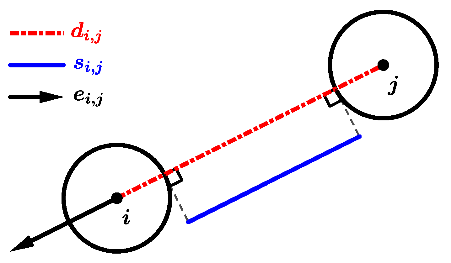
2.1. How to Quantify Contact among Pedestrians

The collision-free velocity model for pedestrian dynamics is used in this work to simulate the movement of customers in the supermarket. It is composed of a direction sub-model and a speed sub-model, and can be described as

$${\dot{X}}_i(X_i,X_j,\cdots )={\overrightarrow{e}}_i(X_i,X_j,\cdots )·V_i(X_i,X_j,\cdots ),$$

(1)

where $X_i$, ${\overrightarrow{e}}_i$, and $V_i$ are the position, moving direction, and moving speed, respectively.

The direction sub-model calculates the moving direction ${\overrightarrow{e}}_i$ for pedestrian i as

$${\overrightarrow{e}}_i=u·\left({\overrightarrow{e}}_i^0+\sum _{j\in N_i}k·exp\left(\frac{-s_{i,j}}{D}\right)·{\overrightarrow{e}}_{i,j}+{\overrightarrow{w}}_i\right),$$

(2)

where u is a normalization constant such that $\parallel {\overrightarrow{e}}_i\parallel =1$. The new direction is decided by three different components. The first component is the ${\overrightarrow{e}}_i^0$, which is an unit vector representing the desired moving direction of the pedestrian i. The second component is the effect from other pedestrians belonging to $N_i$, which is the set that contains all the neighbors who affect the moving direction of pedestrian i. The magnitude of the effect from these neighbors is a function of $s_{i,j}$, which is the distance between the edges of pedestrian i and j along the line connecting their positions. Coefficients $k>0$ and $D>0$ are used to calibrate the function accordingly. The direction of the effect from pedestrian j to i is denoted by ${\overrightarrow{e}}_{i,j}$, which is a unit vector point from the position of pedestrian j to pedestrian i. The definitions of $s_{i,j}$ and ${\overrightarrow{e}}_{i,j}$ are shown in Figure 1. The last part is ${\overrightarrow{w}}_i$, which is the effect from walls and obstacles in the building.

The speed sub-model calculates the moving speed $V_i$ for pedestrians i as

$$V_i=min\left\{V_i^0,max\left\{0,\frac{s_i}{T}\right\}\right\},$$

(3)

where $V_i^0$ is the desired moving speed of pedestrian i, $s_i$ is the collision-free moving spacing of pedestrian i in the moving direction ${\overrightarrow{e}}_i$, and coefficient $T>0$ is used to adjust the speed according to the gap between two pedestrians. A more detailed definition of the model can be found in [21].

The distance among pedestrians changes with time while they are moving in space. We assume that small distances lead to a bigger contact index. Therefore, the index $C_i\left(t\right)$, representing the contact degree of pedestrian i with its neighbors at time t, is defined as

$$C_i\left(t\right)=\sum _{j\in N_i}exp\left(-d_{i,j}\left(t\right)\right),$$

(4)

where $d_{i,j}$ is the distance between the position of pedestrians i and j, see Figure 1.

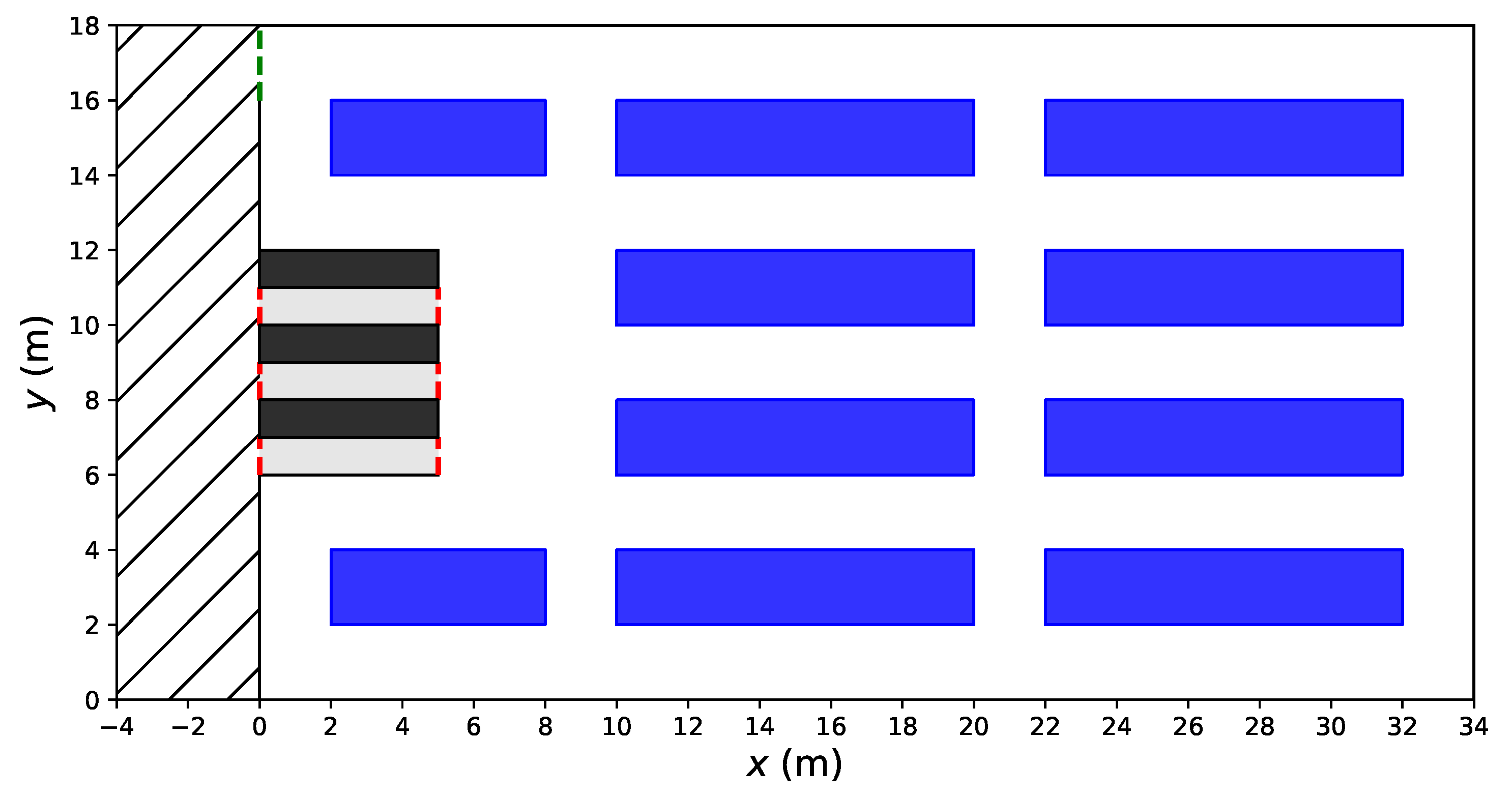
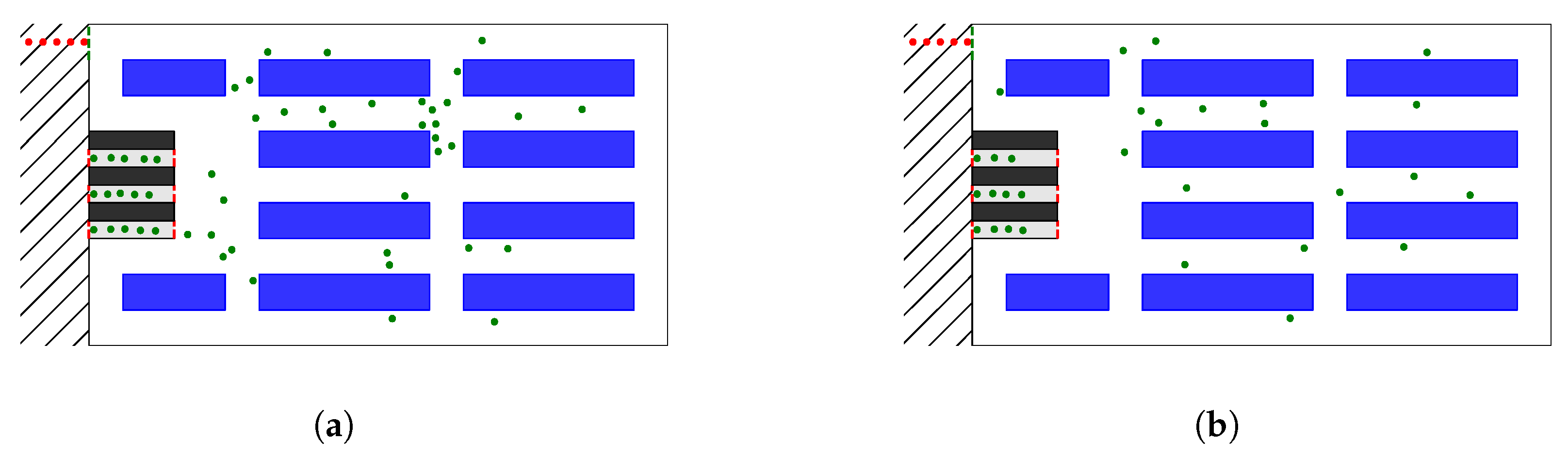
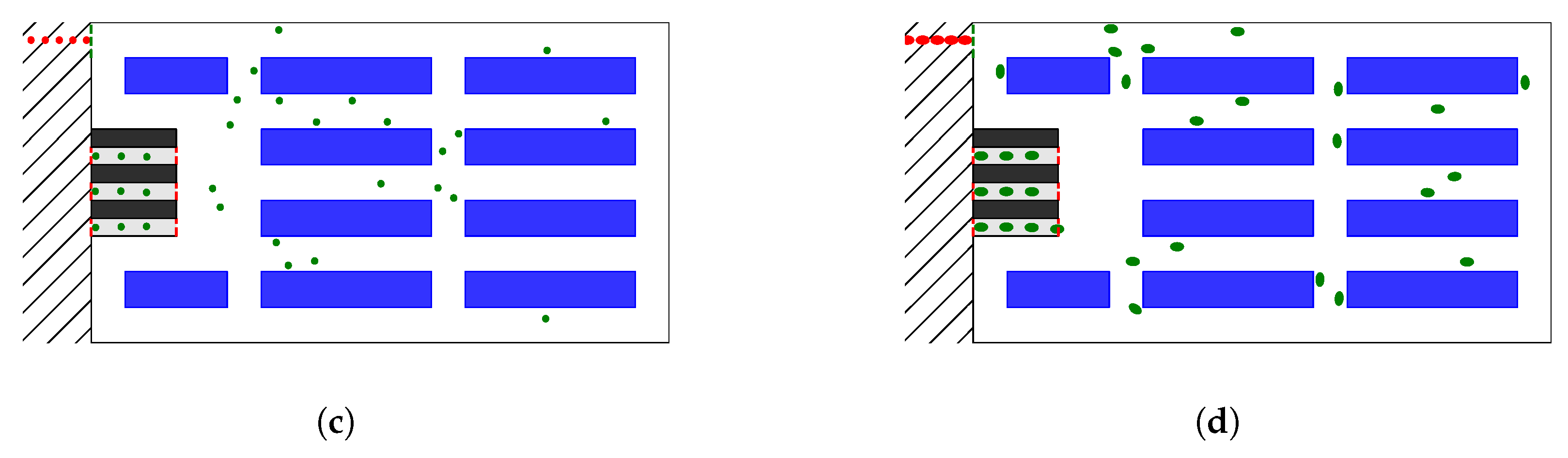
2.2. Simulation of Shopping Behavior in the Supermarket

A fictive supermarket scenario, as shown in Figure 2, is built based on a real supermarket nearby the city Jülich in Germany to simulate several scenarios. It represents the typical structure of a medium-sized supermarket in Germany. The supermarket is 34 m long and 18 m wide. It is composed of three different areas: a checkout, a shopping, and an outside area.

The checkout area includes three counters $5\times 1{\mathrm{m}}^2$ (in black) and three corridors (in gray), while the shopping area includes 10 goods shelves. The sizes of the far left two shelves are $6\times 2{\mathrm{m}}^2$ and the sizes of other shelves are $10\times 2{\mathrm{m}}^2$. Except the area in front of the checkout area, the widths of the walking paths are 2 m. The entrance is located in the upper left corner of the supermarket (green dashed segments). The exits from the shopping area to the checkout area and the exits from checkout area to outside are all marked with red dash segments.

We perform the simulations with a total of M customers. Hereby, P persons are generated outside the supermarket every minute until all the M customers are generated. The generated customers enter the supermarket from the entrance and move in the shopping area. Each customer is assigned a random goal within the supermarket after entering the supermarket. After reaching the goal, the customer is assigned another random goal until the time spent in the shopping area is longer than $t_i^{\mathrm{shop}}$, the shopping time for customers.

As introduced before, there are three counters in the checkout area, which means customers have three choices after finishing the shopping. We assume customers prefer to check out at the counter with the fewest customers. Customers who choose the same counter check out one by one in the order of entering the corridor. The time spent for checking out $t_i^{\mathrm{check}}$ is proportional to the shopping time and is defined as

$$t_i^{\mathrm{check}}=\alpha ·t_i^{\mathrm{shop}},$$

(5)

where $\alpha <1$ is a parameter. Finally, after checking out, the customers leave the supermarket.

Besides the basic movement of customers, the behavior of customers is influenced by the measures adopted by the supermarket. Therefore, these measures are considered into the basic movement model. We introduce three main measures commonly used in supermarkets nowadays.

The first measure is setting a limitation for the maximal number of customers in the supermarket. This is realized by introducing a new parameter $L_{\max }$ in our model, which is the max allowable number of customers in the supermarket at the same time. Customers can only enter the supermarket when the number of persons inside the supermarket does not exceed the threshold $L_{\max }$. Otherwise, customers have to wait outside.

The second measure is asking customers to keep social distance to each other. From daily observations in supermarkets, the social distance rule is well maintained in the checkout area, but cannot be maintained in a strict manner in the shopping area. Therefore, compared with simulations without the social distance rule, a larger value of D in Equation (2) is adopted to enforce larger distances among pedestrians.

Besides, to simulate the queuing of customers, a modified speed sub-model as following is used when customers are in the checkout area.

$$V_i=min\left\{V_i^0,max\left\{0,\frac{d_i-d_i^{\mathrm{wait}}}{T}\right\}\right\}.$$

(6)

In the modified speed sub-model, $d_i$ is the distance between positions of customer i and the nearest front customer. $d_i^{\mathrm{wait}}$ is the distance that customer i wants to keep with the nearest front customer. The expression of $d_i^{\mathrm{wait}}$ is

$$d_i^{\mathrm{wait}}=max\left\{d_{\mathrm{rule}},\beta ·t_i^{\mathrm{shop}}\right\},$$

(7)

where $d_{\mathrm{rule}}$ is the social distance adopted and $\beta$ is a parameter.

When there is no social distance rule, the distance between the customers in the checkout area is decided by the shopping time, as we assume that longer shopping times correspond to more space for putting purchased good on the conveyor belt. When the social distance measure is taken, customers maintain at least $d_{\mathrm{rule}}$ distances with each other even when they purchase few items in the market.

The last measure is requiring customers to enter the supermarket with a shopping cart. In our simulations, customers are represented by circles with a radius r. Considering that shopping carts increase the space occupied by each customer in the supermarket, a bigger ellipse is used to represent the customers with shopping carts. The length of the semi-major axis in the moving direction is a, and the length of semi-minor axis is b.

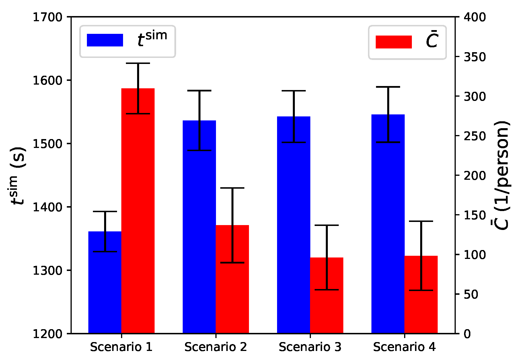
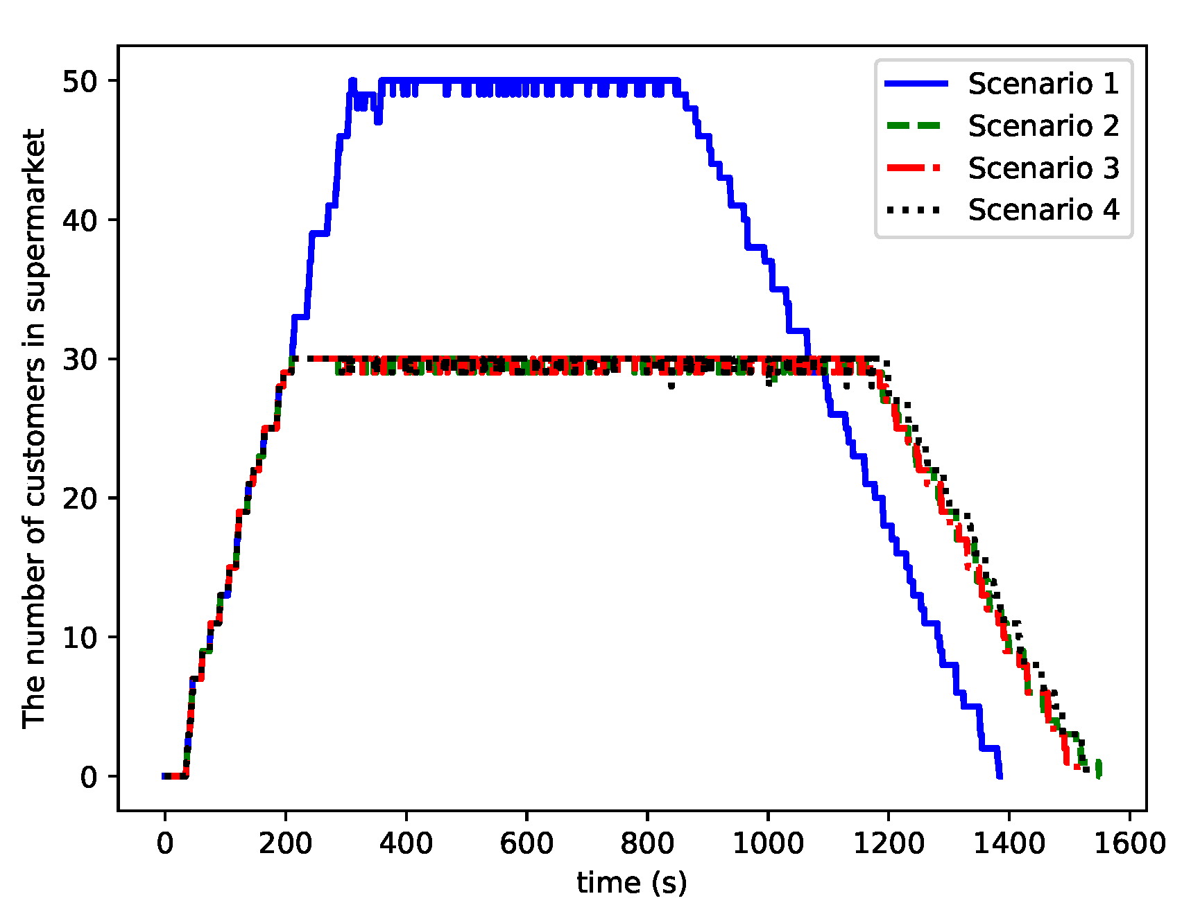
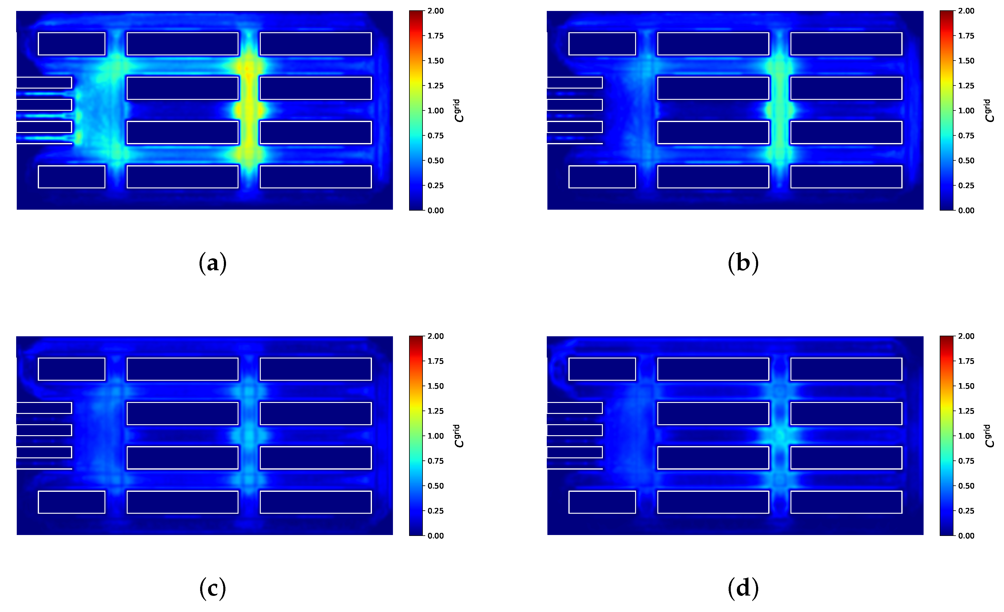
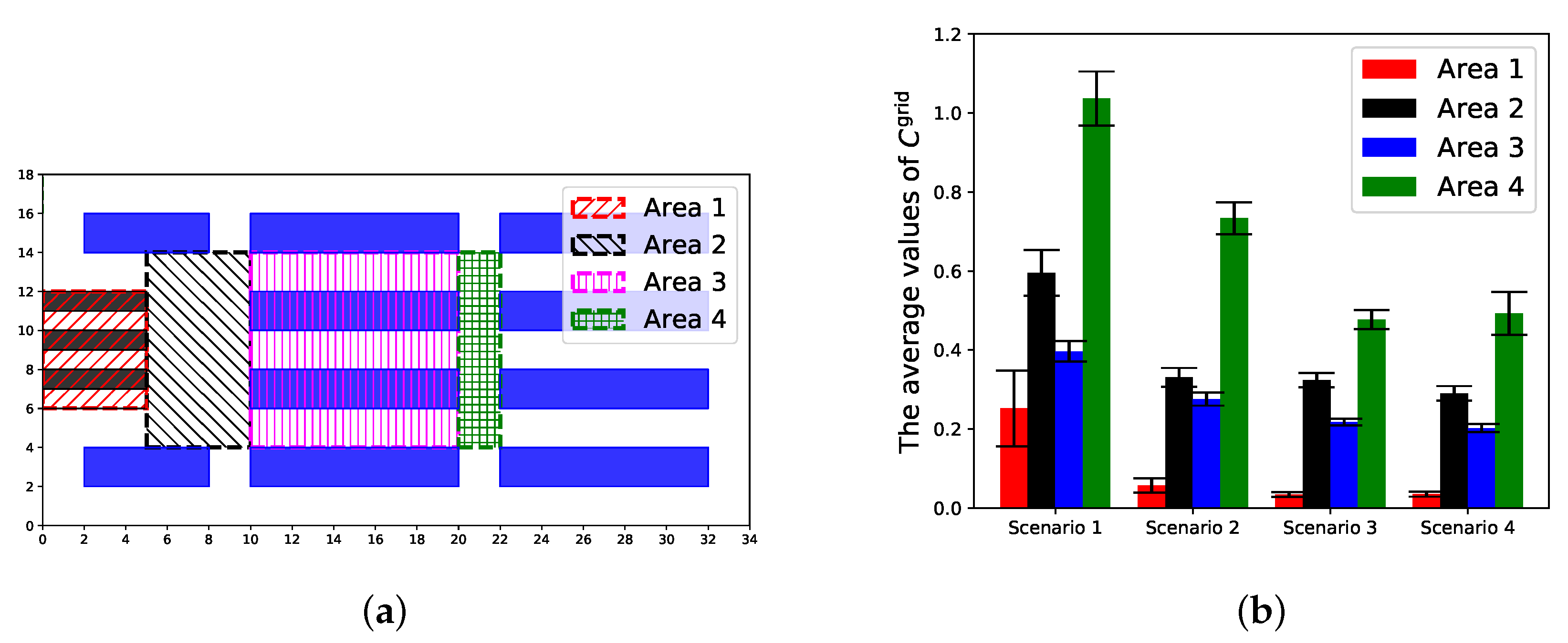
3. Simulation Results

To explore if the measures taken by the supermarkets are efficient in reducing the contact among customers, the simulations are implemented in the geometry shown in Figure 2 with four different scenarios. For all cases, we use the following parameter values in

Table 1. The same parameters in all four scenarios. k (Equation (2)) is the parameter to calibrate the strength of the impact from other pedestrians, T (Equations (3) and (6)) is the parameter to calibrate the speed according to the gap between two pedestrians, $\alpha$ (Equation (5)) is the parameter to calibrate the checkout time according to the shopping time, $\beta$ (Equation (7) is the parameter to calibrate the distance between customers in checkout area according to the shopping time, M is the total number of customers generated in the simulation, P is the number of customers generated every minute, $V_i^0$ (Equations (3) and (6)) is the desired moving speed of customers, and $t_i^{\mathrm{shop}}$ is the shopping time of customers.

Parameters	Values
k	8
T (s)	1
$\alpha$	0.1
$\beta$ (m/s)	0.003
M (person)	100
P (person/min)	10
$V_i^0$ (m/s)	N∼$(1.34,{0.26}^2)$
$t_i^{\mathrm{shop}}$ (s)	N∼$(300,{50}^2)$

. We assumed reasonable values for the desired moving speeds and the shopping times of customers, which are normally distributed for heterogeneity. The mean and standard deviation of the desired moving speeds refer to the free walking speed of pedestrians [22,23]. The other values in Table 1 are kept constant to guarantee the justification of the comparisons between different scenarios.

The differences among the settings of these four scenarios are shown in

Table 2. The setting of four scenarios in this work. $L_{\max }$ is the max allowable number of customers in the supermarket at the same time, $d_{\mathrm{rule}}$ is the social distance, and D (Equation (2)) is the parameter to calibrate the scale of the impact from other pedestrians.

Scenario ID	${\mathit{L}}_{\mathbf{max}}$ (Person)	${\mathit{d}}_{\mathbf{rule}}$ (m)	D (m)	Need Shopping Cart
1	50	0	0.1	No
2	30	0	0.1	No
3	30	1.5	0.3	No
4	30	1.5	0.3	Yes

. A complete list of all parameters choices in the four scenarios is given in

Table A1. The complete list of all parameters choices in four scenarios with the explanation.

Parameters	Explanation	Values
		Scenario 1	Scenario 2	Scenario 3	Scenario 4
k	The parameter to calibrate the strength of the impact from other pedestrians (Equation (2))	8
D	The parameter to calibrate the scale of the impact from other pedestrians (Equation (2))	0.1	0.1	0.3	0.3
$V_i^0$ (m/s)	The desired moving speed of customers (Equations (3) and (6))	N∼$(1.34,{0.26}^2)$
T (s)	The parameter to calibrate the speed according to the gap between two pedestrians (Equations (3) and (6))	1
$\alpha$	The parameter to calibrate the checkout time according to the shopping time (Equation (5))	0.1
$\beta$ (m/s)	The parameter to calibrate the distance between customers in checkout area according to the shopping time (Equation (7))	0.03
M (person)	The total number of customers generated in the simulation	100
P (person/min)	The number of customers generated every minute	10
$t_i^{\mathrm{shop}}$ (s)	The shopping time of customers	N∼$(300,{50}^2)$
$d_{\mathrm{rule}}$ (m)	The social distance	0	0	1.5	1.5
$L_{\max }$ (person)	The max allowable number of customers in the supermarket at the same time	50	30	30	30
Need shopping cart	Decide the shape of customers in simulations (customers without shopping cart are represented by circles with r = 0.2 m, customers with shopping cart are represented by ellipses with semi-axes $a=0.4$ m and $b=0.25$ m.)	No	No	No	Yes
$\Delta t$ (s)	The size of time-step in simulations	0.05

(Appendix A).

The snapshots of each scenario are shown in Figure 3. The customers are represented by circles with r = 0.2 m in scenarios 1, 2, and 3, where customers can enter the supermarket without a shopping cart. In scenario 4, customers enter the supermarket with shopping carts, therefore they are represented by ellipses with semi-axes $a=0.4$ m and $b=0.25$ m. Customers inside the supermarket are in green whereas customers outside are in red.

Supermarkets take measures to reduce the contact among customers, but these measures may result in a decrease in the service efficiency. Two quantities are chosen to study the trade-off between the efficiency of the supermarket and the effectiveness of the measures: The first one is $t^{\mathrm{sim}}$, which is the time spent by all the M customers in the supermarket. $t^{\mathrm{sim}}$ reflects the efficiency of the supermarket. It can be represented by

$$t^{\mathrm{sim}}=t^{\mathrm{last}}-t^{\mathrm{first}},$$

(8)

where $t^{\mathrm{first}}$ is the time when the first customer enters the supermarket, and $t^{\mathrm{last}}$ is the time when the last customer leaves the supermarket. The second one is the average contact degree of all the M customers, which is defined as

$$\overline{C}=\frac{1}{M}·{\int }_{t^{\mathrm{first}}}^{t^{\mathrm{last}}}\sum _{i=1}^M{C}_i\left(t\right)dt.$$

(9)

If customer i is outside the supermarket, $C_i$ is equal to zero. A reasonable measure should reduce $\overline{C}$ as much as possible without increasing $t^{sim}$ significantly.

The simulations of this work are performed using JuPedSim [24], which is an open framework for simulating and analyzing the dynamics of pedestrians. The simulations are executed on a standard computer (Inter(R) Core(TM) CPU of 2.50 GHZ) with Euler scheme using a time step $\Delta t=0.05$s. The update of the customers is parallel in each time-step. We run simulations in each scenario for 30 times. Then, we calculated the mean value and standard deviation of $t^{\mathrm{sim}}$ and $\overline{C}$, which are shown in Figure 4.

Hypothesis testing is implemented before comparing the results of different scenarios. The null hypothesis is set as there is no significant difference between the results of two compared scenarios. The Shapiro–Wilks test is performed first to test the normality of the differences between the results of two scenarios. Since all the differences satisfy the condition of normality ($p_1$ is greater than 0.05), we can perform the Paired t-test for all the comparisons. The null hypothesis is accepted when $p_2$ is greater than 0.05. The results of Shapiro–Wilks test and Paired t-test are shown in

Table 3. The result of Shapiro–Wilks test and Paired t-test. ($S1$ means the result from scenario 1.)

		Mean	Standard Deviation	Shapiro–Wilks Test			Paired t-Test
				$\mathit{W}$	${\mathit{p}}_{\mathbf{1}}$		$\mathit{t}$	${\mathit{p}}_{\mathbf{2}}$
$t_{sim}$	$S1–S2$	−175.3000	26.8790	0.9798	0.8200		−35.1211	0.0000
	$S2–S3$	−6.1125	16.1472	0.9666	0.4497		−2.0385	0.0507
	$S3–S4$	−3.2083	18.0953	0.9709	0.5639		−0.9548	0.3476
$\overline{C}$	$S1–S2$	172.7929	11.7533	0.9828	0.8938		79.1711	0.0000
	$S2–S3$	40.5942	5.8819	0.9755	0.6980		37.1660	0.0000
	$S3–S4$	−2.1007	7.5094	0.9426	0.1070		−1.5065	0.1428

.

From scenario 1 to scenario 4, the protective measures adopted by the supermarket become stricter. Comparing scenario 1 and scenario 2, scenario 2 has smaller $L_{max}$ than scenario 1. The values of $p_2$ for $t_{sim}$ and $\overline{C}$ are both less than 0.05, showing a significant difference between the results of these two scenarios. From scenario 1 to scenario 2, the mean value of $\overline{C}$ decreases roughly $56\%$, and the mean value of $t^{\mathrm{sim}}$ increases roughly $13\%$. In conclusion, restricting the number of customers in the supermarket is an effective measure to reduce the contact among customers with a slightly reduced efficiency of the supermarket.

Scenario 2 and scenario 3 have the same $L_{\max }$, but the social distance rule is adopted in scenario 3. Since the value of $p_2$ for $t_{sim}$ is greater than 0.05, we can say there is no significant difference between $t_{sim}$ of these two scenarios. For $\overline{C}$, the value of $p_2$ is less than 0.05. The mean value of $\overline{C}$ decreases nearly $29\%$ from scenario 2 to scenario 3. Therefore, social distance rule is also effective to reduce the contact, and hardly affect the efficiency of the supermarket.

In scenario 4, the shopping cart is required for entering the supermarket. Compared with scenario 3, the values of $p_2$ for $t_{sim}$ and $\overline{C}$ are both greater than 0.05. Therefore, it seems that the shopping cart rule has limited effect with respect to reducing the contact, although this rule can reduce the workload of counting customers, since the supermarket can limit the number of people in the supermarket by placing a shopping cart with a quantity of $L_{\max }$.

In addition to the two quantities, the spatial distribution of the contact among customers in the supermarket is investigated. The steady state of each scenario is identified first, which is defined as the status that the number of customers in the supermarket reaches $L_{\max }$. For each scenario, one run is picked out to show the steady states. The steady states of these four scenarios correspond to the flat regions of four lines in Figure 5. The steady areas of scenarios 2, 3, and 4 are almost overlapped, as the value of $L_{\max }$ are the same. The vertical axis represents the number of customers in the supermarket. The oscillation of the steady state is caused by the time gap between customers entering and leaving the supermarket. The start time and the end time of the steady state is defined as $t^{\mathrm{start}}$ and $t^{\mathrm{end}}$, respectively.

The geometry of the supermarket is divided into regular grids of size $0.2\times 0.2{\mathrm{m}}^2$, and an index $C^{\mathrm{grid}}$ is calculated for each grid according to

$$C^{\mathrm{grid}}=\frac{{\int }_{t^{\mathrm{start}}}^{t^{\mathrm{end}}}{\sum }_{i\in G}{C}_i\left(t\right)dt}{{\int }_{t^{\mathrm{start}}}^{t^{\mathrm{end}}}{\sum }_{i\in G}dt},$$

(10)

where G is the set containing all the customers in the grid. We calculate the mean value of $C^{\mathrm{grid}}$ in each grid with the 30 times simulations of each scenario. The distributions of $C^{\mathrm{grid}}$ in the supermarket for four scenarios are shown in Figure 6.

A qualitative observation shows that the distribution of $C^{\mathrm{grid}}$ changes with the measures taken by the supermarket. The same conclusions as before can be obtained, for instance, restricting the number of customers and social distance rule are useful to reduce the contact among customers, and the shopping cart rule is not effective.

The four profiles in Figure 6 also show that the values of $C^{\mathrm{grid}}$ differ depending on different parts of the supermarket. Therefore, in Figure 7a four areas in the supermarket are specified, and the average values of $C^{\mathrm{grid}}$ in these areas are calculated. The grids which are located in the obstacles (e.g., counters and goods shelves) are ignored in the calculation, as the values of $C^{\mathrm{grid}}$ in the obstacle areas are always equal to zero. The mean values and standard deviations of 30 times simulations for four scenarios are compared in Figure 7b.

The same hypothesis testing is implemented for following comparisons. Paired t-test is performed when the difference between two scenarios satisfy the condition of normality. Otherwise, Wilcoxon signed-rank test is used. The testing results are shown in

Table 4. The testing result of comparisons for different areas in the supermarket. ($S1$ means the result from scenario 1.)

		Mean	Standard Deviation	Shapiro–Wilks Test			Paired t-Test (Wilcoxon)
				$\mathit{W}$	${\mathit{p}}_{\mathbf{1}}$		$\mathit{t}\left(\mathit{W}\right)$	${\mathit{p}}_{\mathbf{2}}$
Area 1	$S1–S2$	0.1952	0.0907	0.6739	0.0000		0.0000	0.0000
	$S2–S3$	0.0229	0.0135	0.9247	0.0355		0.0000	0.0000
	$S3–S4$	−0.0009	0.0052	0.9837	0.9140		−0.8889	0.3814
Area 2	$S1–S2$	0.2646	0.0663	0.9414	0.0994		21.5000	0.0000
	$S2–S3$	0.0070	0.0285	0.9705	0.5527		1.3228	0.1962
	$S3–S4$	0.0336	0.0257	0.9638	0.3851		7.0483	0.0000
Area 3	$S1–S2$	0.1210	0.0316	0.9822	0.8799		20.5898	0.0000
	$S2–S3$	0.0582	0.0167	0.9939	0.9996		18.7725	0.0000
	$S3–S4$	0.0153	0.0133	0.9488	0.1566		6.1786	0.0000
Area 4	$S1–S2$	0.3027	0.0774	0.9711	0.5688		21.0676	0.0000
	$S2–S3$	0.2570	0.0520	0.9908	0.9946		26.6224	0.0000
	$S3–S4$	−0.0157	0.0587	0.9714	0.5795		−1.4439	0.1595

.

The common point of these four scenarios is the average values of $C^{\mathrm{grid}}$ in Area 2 and Area 4 are higher than in Area 1 and Area 3. The reason is that crossing structures are exist in Area 2 and Area 4. Customers in these crossing areas can move in more directions, thus increasing the likelihood of congestion, especially when the number of customers in the supermarket is high.

More information can be obtained by combining Figure 7b and Table 4. Restricting the number of customers decreases the value of $C^{\mathrm{grid}}$ in all four areas. The social distance rule also reduces the contact of customers in Area 1, Area 3 and Area 4, but has no effect in Area 2. As for the shopping cart rule, it has a little influence in Area 2 and Area 3, and no effect in Area 1 and Area 4.

4. Conclusions

Supermarkets are closely related to people’s daily life. During the COVID-19 period, a series of measures are adopted in supermarkets to slow down the propagation of the disease. The effectiveness of these measures are investigated in this paper. The contact degree among customers is treated as the standard for comparing different measures. Simulations of several scenarios corresponding to different measures taken by supermarkets are performed.

We run simulations in each scenario for 30 times and implement hypothesis testing. Although the supermarket scenarios used in this work is simplified and the behavior of customers in our simulations are based on several assumptions, the following results can be obtained by comparing the accumulation of the time spent by all the customers in the supermarket and the average contact degree of these costumers. The limitation on the number of customers in the supermarket slightly reduces the efficiency of the supermarket, but significantly reduces the contact among customers. The social distance rule is also effective at reducing the contact among customers. However, the shopping cart rule has little effect in reducing the contact among customers.

Moreover, the spatial distribution of the contact between customers in the supermarket shows that the contact in the areas with crossing structure is obviously higher than in other areas. Therefore, reducing the crossing area in the supermarket may be an effective measure to reduce the contact among customers.

In summary, supermarkets should continue to limit the number of customers and require customers to maintain a minimum social distance. Besides, supermarkets can change the layout to reduce the crossing area.

The work in this paper only focus on the contact among people using on a velocity-based model, but has potential to be extended to an epidemiology model by combining the knowledge and data about the spread COVID-19 into the movement model.

The results of this work may change with the structure of the fictive supermarket scenario and the behavior of customers in simulations, but nonetheless we believe that the framework presented in this study can evaluate the effectiveness of control measures in indoors scenarios.

Future research will focus on the dependence of our results on the structure of scenarios (like the width of walking paths, the number of counters in the checkout area) and behavior of customers (i.e., the shopping time $t^{\mathrm{shop}}$ and the desired moving speed $V_i^0$). Besides, the validation of both movement and behavioral models in this work will be proceed.

References

1. World Health Organization. WHO Timeline—COVID-19. Available online: https://www.who.int/news-room/detail/27-04-2020-who-timeline---covid-19 (accessed on 29 June 2020).
2. World Health Organization. WHO Coronavirus Disease (COVID-19) Dashboard. Available online: https://covid19.who.int/ (accessed on 29 June 2020).
3. World Health Organization. Q&A on Coronaviruses (COVID-19). Available online: https://www.who.int/emergencies/diseases/novel-coronavirus-2019/question-and-answers-hub/q-a-detail/q-a-coronaviruses (accessed on 29 June 2020).
4. World Health Organization. Novel Coronavirus (2019-nCoV) Advice for the Public. Available online: https://web.archive.org/web/20200126025750/https://www.who.int/emergencies/diseases/novel-coronavirus-2019/advice-for-public (accessed on 29 June 2020).
5. Prem, K.; Liu, Y.; Russell, T.W.; Kucharski, A.J.; Eggo, R.M.; Davies, N.; Flasche, S.; Clifford, S.; Pearson, C.A.; Munday, J.D.; et al. The effect of control strategies to reduce social mixing on outcomes of the COVID-19 epidemic in Wuhan, China: A modelling study. Lancet Public Health 2020, 5, e261–e270. [Google Scholar] [CrossRef] [Green Version]
6. Kraemer, M.U.; Yang, C.H.; Gutierrez, B.; Wu, C.H.; Klein, B.; Pigott, D.M.; Du Plessis, L.; Faria, N.R.; Li, R.; Hanage, W.P.; et al. The effect of human mobility and control measures on the COVID-19 epidemic in China. Science 2020, 368, 493–497. [Google Scholar] [CrossRef] [PubMed] [Green Version]
7. Tian, H.; Liu, Y.; Li, Y.; Wu, C.H.; Chen, B.; Kraemer, M.U.; Li, B.; Cai, J.; Xu, B.; Yang, Q.; et al. An investigation of transmission control measures during the first 50 days of the COVID-19 epidemic in China. Science 2020, 368, 638–642. [Google Scholar] [CrossRef] [PubMed] [Green Version]
8. D’Orazio, M.; Bernardini, G.; Quagliarini, E. Sustainable and resilient strategies for touristic cities against COVID-19: An agent-based approach. arXiv 2020, arXiv:2005.12547. [Google Scholar]
9. Szczepanek, R. Analysis of pedestrian activity before and during COVID-19 lockdown, using webcam time-lapse from Cracow and machine learning. PeerJ 2020, 8, e10132. [Google Scholar] [CrossRef] [PubMed]
10. Ronchi, E.; Lovreglio, R. EXPOSED: An occupant exposure model for confined spaces to retrofit crowd models during a pandemic. arXiv 2020, arXiv:2005.04007. [Google Scholar] [CrossRef] [PubMed]
11. D’Orazio, M.; Bernardini, G.; Quagliarini, E. A Probabilistic Model to Evaluate the Effectiveness of Main Solutions to COVID-19 Spreading in University Buildings according to Proximity and Time-Based Consolidated Criteria. Res. Sq. 2020. [Google Scholar] [CrossRef]
12. Kucharski, A.J.; Russell, T.W.; Diamond, C.; Liu, Y.; Edmunds, J.; Funk, S.; Eggo, R.M.; Sun, F.; Jit, M.; Munday, J.D.; et al. Early dynamics of transmission and control of COVID-19: A mathematical modelling study. Lancet Infect. Dis. 2020, 20, 553–558. [Google Scholar] [CrossRef] [Green Version]
13. Berger, D.W.; Herkenhoff, K.F.; Mongey, S. An Seir Infectious Disease Model with Testing and Conditional Quarantine; Technical report; National Bureau of Economic Research: Cambridge, MA, USA, 2020. [Google Scholar]
14. Barbarossa, M.V.; Fuhrmann, J.; Meinke, J.H.; Krieg, S.; Varma, H.V.; Castelletti, N.; Lippert, T. The impact of current and future control measures on the spread of COVID-19 in Germany. medRxiv 2020. [Google Scholar] [CrossRef]
15. Hou, C.; Chen, J.; Zhou, Y.; Hua, L.; Yuan, J.; He, S.; Guo, Y.; Zhang, S.; Jia, Q.; Zhao, C.; et al. The effectiveness of quarantine of Wuhan city against the Corona Virus Disease 2019 (COVID-19): A well-mixed SEIR model analysis. J. Med. Virol. 2020. [Google Scholar] [CrossRef] [PubMed] [Green Version]
16. Iwata, K.; Miyakoshi, C. A Simulation on Potential Secondary Spread of Novel Coronavirus in an Exported Country Using a Stochastic Epidemic SEIR Model. J. Clin. Med. 2020, 9, 944. [Google Scholar] [CrossRef] [PubMed] [Green Version]
17. Fang, Z.; Huang, Z.; Li, X.; Zhang, J.; Lv, W.; Zhuang, L.; Xu, X.; Huang, N. How many infections of COVID-19 there will be in the “Diamond Princess”-Predicted by a virus transmission model based on the simulation of crowd flow. arXiv 2020, arXiv:2002.10616. [Google Scholar]
18. D’Orazio, M.; Bernardini, G.; Quagliarini, E. How to restart? An agent-based simulation model towards the definition of strategies for COVID-19 “second phase” in public buildings. arXiv 2020, arXiv:2004.12927. [Google Scholar]
19. Kai, D.; Goldstein, G.P.; Morgunov, A.; Nangalia, V.; Rotkirch, A. Universal masking is urgent in the covid-19 pandemic: Seir and agent based models, empirical validation, policy recommendations. arXiv 2020, arXiv:2004.13553. [Google Scholar]
20. Xiao, Y.; Yang, M.; Zhu, Z.; Yang, H.; Zhang, L.; Ghader, S. Modeling indoor-level non-pharmaceutical interventions during the COVID-19 pandemic: A pedestrian dynamics-based microscopic simulation approach. arXiv 2020, arXiv:2006.10666. [Google Scholar]
21. Xu, Q.; Chraibi, M.; Tordeux, A.; Zhang, J. Generalized collision-free velocity model for pedestrian dynamics. Phys. A Stat. Mech. Appl. 2019, 535, 122521. [Google Scholar] [CrossRef] [Green Version]
22. Bosina, E.; Weidmann, U. Estimating pedestrian speed using aggregated literature data. Phys. A Stat. Mech. Appl. 2017, 468, 1–29. [Google Scholar] [CrossRef]
23. Buchmueller, S.; Weidmann, U. Parameters of pedestrians, pedestrian traffic and walking facilities. IVT Schriftenreihe 2006, 132, 15. [Google Scholar] [CrossRef]
24. Wagoum, A.U.K.; Chraibi, M.; Zhang, J.; Lämmel, G. JuPedSim: An open framework for simulating and analyzing the dynamics of pedestrians. In Proceedings of the 3rd Conference of Transportation Research Group of India, West Bengal, India, 17–20 December 2015. [Google Scholar]
Figure 1. The definition of s i , j , d i , j and e i , j . s i , j is the distance between the edges of pedestrian i and j along the line connecting their positions, d i , j is the distance between the position of pedestrians i and j, and e i , j is a unit vector point from the position of pedestrian j to pedestrian i.
Sustainability 12 09385 g001
Figure 2. The geometrical structure of the supermarket used in the simulations, the outside area of the supermarket is filled with hatch lines.
Sustainability 12 09385 g002
Figure 3. The snapshots of four scenarios; customers inside the supermarket are in green, whereas customers outside are in red. (a) Scenario 1. (b) Scenario 2. (c) Scenario 3. (d) Scenario 4.
Sustainability 12 09385 g003aSustainability 12 09385 g003b
Figure 4. The comparison of t sim (time spend by all customers) and C ¯ (average contact degree of all customers) for four scenarios, the error bars show the standard deviation.
Sustainability 12 09385 g004
Figure 5. The steady states of the four scenarios.
Sustainability 12 09385 g005
Figure 6. The distributions of C grid in the supermarket for four scenarios. (a) Scenario 1. (b) Scenario 2. (c) Scenario 3. (d) Scenario 4.
Sustainability 12 09385 g006
Figure 7. The average values of C grid in specified areas. (a) The locations of these areas. (b) The comparison of average values; the error bars show the standard deviation.
Sustainability 12 09385 g007