Article

The Analysis Performance of a Grid-Connected 8.2 kWp Photovoltaic System in the Patagonia Region

1
C.E.R.E., Faculty of Engineering, University of Magallanes, Punta Arenas 6200000, Chile
2
Department of Electrical Engineering, Faculty of Engineering, Universidad de Talca, Campus Curicó 3344158, Chile
3
Faculty of Engineering, The University of Nottingham, Nottingham NG7 2RD, UK
*
Author to whom correspondence should be addressed.
Sustainability 2020, 12(21), 9227; https://doi.org/10.3390/su12219227
Submission received: 9 September 2020 / Revised: 31 October 2020 / Accepted: 2 November 2020 / Published: 6 November 2020
(This article belongs to the Special Issue Photovoltaic Power)

Abstract

:
Solar PV structures for locations at high latitudes in the Northern and Southern Hemispheres are increasingly in the spotlight. The work reported in this paper analyses the behaviour of a grid-connected 8.2 kWp photovoltaic system to either feed on-site electrical loads (a public institution, Corporación Nacional Forestal (CONAF), located 5.5 km south of Punta Arenas, lat. 53° S) or to feed into the electrical grid when the photovoltaic system generation is higher than the on-site load demand. The system simulation uses the PVSyst software with Meteonorm derived and measured climate information sets (ambient temperature, solar irradiation and wind speed). The agreement between the simulated and measured energy yield is analysed including the evaluation of the optimal generation energy of the PV array, the energy that is fed into the network, the performance ratio, and the normalised energy generation per installed kWp. The PV system considered in this work generates 7005.3 kWh/year, out of which only 6778 kWh/year are injected into the grid. The measured annual performance ratio is around 89%. The normalised productions of the inverter output or final system yield, i.e., useful energy, is 3.6 kWh/kWp/day. The measured annual average capacity factor obtained from this study is 15.1%. These performance parameters will encourage greater use of photovoltaic technology in the Chilean Patagonia region.

1. Introduction

The National Electrical Grid (SEN) in Chile is the main electrical system in the country and represents about 99% of the installed capacity in Chile. The electrical system of Magallanes is far smaller and has several unconnected subsystems due to geographical isolation, making the area very expensive to interconnect with the SEN. Electricity generation in Magallanes is mainly from natural gas with a minor contribution from diesel. This is considered a vulnerability due to the dependence on fossil resources, which are finite [1].
It is well known that Patagonia is attractive for wind power installations as a result of its excellent wind resource. However, over the last few years, solar energy has received attention in Magallanes, due to a rapid price reduction in PV technology and the increasing awareness of sustainable energy in these southernmost settlements in the world. As a result of the Magallanes energy policy, the government is committed to increasing the utilisation of the cleanest energy supplies, wind, marine and solar energy, as the way to move toward a renewable energy matrix. Punta Arenas is in the southern area of America, in a region with low sunshine duration levels with generally lower solar irradiation than many other areas. The latitude and longitude of Punta Arenas is 53° S and 71° W, respectively, and PV installations in Magallanes tend to be dominated by domestic and stand-alone systems [2].
A schematic for a generalised grid-connected photovoltaic system is shown in Figure 1. The electrical energy produced by such a photovoltaic system can be fed into the electrical network, according to pre-defined quality and reliability characteristics and without damaging the network’s normal operation. The PV array is connected to the network using an inverter, which transforms the DC output of the array PV panels to an AC output waveform matched to the voltage and frequency of the local network. It should be noted that the system as shown in Figure 1 does not include any facility for the storage of energy; this is the usual configuration of many current grid-connected photovoltaic systems [3].
To predict the behaviour of a PV system, its working characteristics under different climates, the varying mixtures of components and different installation schemes, advanced computer-based simulation studies are required [4]. In [5], a solar photovoltaic design and the associated management software were evaluated, studying their attributes against fifteen key characteristics of solar photovoltaic design and administration criteria. In this work, the system is modelled using PVSyst [6], a widely used computational tool. The real system’s operation is monitored using one year’s data. The main contribution in this work is to obtain the yearly electrical energy yield and associated performance ratio of a photovoltaic system installed in the Magallanes region of Chilean Patagonia.
A performance assessment for the PV systems is used to find the potential for photovoltaic energy production in an area. There are different analyses considering the performance of photovoltaic modules established outdoors across the world [4,7,8,9,10,11,12,13,14,15,16,17]. In [7], a technical and economic evaluation was presented for a selected number of home systems in Palestine, showing a payback in less than five years for a 5 kW system. The same principle was considered in [8,9,10] for a rooftop photovoltaic grid-tied system in Norway, Eastern India and Serbia, respectively. In [11], the PVSyst software was used to compare three technologies of a grid-connected PV system, mono-crystalline, polycrystalline and amorphous, demonstrating that mono-crystalline technology shows better results than polycrystalline, whereas amorphous has the worst performance. Annual energy behaviour indexes for different types of PV technologies have been evaluated under several Moroccan climates [12]. Similarly, in [13], the energy production from two PV technologies was studied in an institutional building in Morocco, evaluating the economic and environmental aspects and comparing them with other PV plants worldwide. Again, technical, economic and environmental aspects of a PV system were considered for a city in Indonesia [14], demonstrating the advantages and challenges for such installations. A comparison between the measured and simulated performance of a grid-connected PV system in South-Africa was presented in [15], showing the vast potential for suitable solar power generation. Sunny and cloudy scenarios were considered in the power quality observations for a PV grid-connected system in Egypt [16], where it was concluded that low solar irradiance has a remarkable impact. Nevertheless, except for the work of Watts et al. [18], there is a lack of accessible data about the current operation and energy production from small grid-connected photovoltaic systems operating in the southern regions of South America. In [19], an assessment and performance analysis of a 28 kWp PV grid-tied system in the Saharan environment was reported. The PV system was monitored over 12 months (March 2017 to February 2018), and the measured data were used to evaluate both the energy efficiency and the output power losses. The article was mainly focused on the impacts of the distribution grid on the annual energy efficiency of the PV system.
Different control strategies have been proposed for the improvement of photovoltaic grid-connected systems. Among them, in [20], a prescribed performance-based adaptive backstepping controller to regulate the active power of the system was proposed. Similarly, with the objective of regulated power quality, in [21], a supercapacitor energy storage system based on a static synchronous compensator was proposed. A predictive control strategy was proposed in [22] where the mathematical model of the system was considered to predict the future performance of the controlled variables, and based on an optimization criterion, the best suitable switching state was applied to the converter. A perturb and observe strategy together with the extremum seeking control was proposed in [23] to maximize the extracted power of a photovoltaic system under any level of weather fluctuations. In [24], a hybrid photovoltaic fuel-cell battery system was described, and this system supplies a small community in Saudi Arabia. The study was focused on the design and sensitivity analysis of the system. Similarly, in [25], a techno-economics and operational performance assessment of a 10 kWp photovoltaic grid-connected plant was conducted using the collected data, simulation, and optimization of the entire system. This was a similar study in comparison to the one proposed in this paper with the difference that this was done in Ethiopia and Saudi Arabia, which are very well known for high solar radiation, and the software used was MATLAB/Simulink and the Hybrid Optimization Model for Electric Renewables (HOMER) software.
The novelty of this paper is the demonstration of the energy production potential of a small-scale grid-connected photovoltaic architecture situated in the Magallanes region of Chile, which is a totally different environment in comparison to the works presented in [24,25]. The results presented are helpful for policy makers, individuals and organisations as they give actual realistic performance characteristics and the potential of the grid-connected photovoltaic architecture in this part of the world. This study’s goals consist of examining the technical feasibility of a solar photovoltaic architecture as an energy supply in the Magallanes region and estimating energy output from the photovoltaic architecture. Additionally, the performance outcomes presented were acquired from field monitoring of the behaviour of a 8.2 kWp PV grid-connected system, which is 5.5 km south of Punta Arenas. Even though Magallanes is characterised by low temperatures, low levels of solar irradiation and strong winds, the results obtained from this system indicate that on-grid photovoltaic systems can be designed to work efficiently and can have a performance that is comparable to similar photovoltaic systems situated in other cities with similar latitudes in the Northern Hemisphere. Because of the good results obtained, this paper presents the incentive to use photovoltaic energy in Patagonia.

2. Behaviour and Viability Analysis of Photovoltaic Solar Systems

This section discusses previous works associated with the operational performance and viability studies of PV solar systems carried out by employing the PVSyst software tool [4,7,11,12,13,14,15]. Three different photovoltaic systems, each of them rated at 5 kW, were analysed in [7]. Examining the measurements of data relating the performance of these systems during two years of operation, in the West Bank region, a mean daily yield of 4.81 kWh/kWp per day, corresponding to a yearly yield of 1756 kWh/kWp, was reported. The main economical outcomes encourage the use of such residential PV systems, considering that the pay-back period for such a system is 4.9 years, and 0.115 US$ is the cost of one kWh produced.
In [11], a comparative and behaviour analysis of three photovoltaic technologies was performed, and their performance was analysed (mono-crystalline, polycrystalline and amorphous). All the panels were linked together to have an installed total capacity of 5.94 kWp on the roof of the Faculty of Science of Tetouan, Morocco. PVSyst was used to simulate the behaviour of these three technologies. The final yield and the energy integrated into the utility from the three panel types were compared using data acquired during 2016. The final yield for each technology was simulated, and the results closely matched the annual reference yield. The monocrystalline technology produced more energy when compared to the rest of the technologies.
Another author modelled a 100 kWp system connected to the grid [4]. The system was also simulated in PVSyst and consisted of 323 Si-poly photovoltaic panels (with a rating of 310 Wp per panel), four solar inverters (20 kW) and weather datasets for solar irradiation, along with an ambient temperature from the PVSyst database for Talangana, India (source: Meteonorm 7.1). Some of the main results for this 100 kWp PV system were a rated generation of 165.38 MWh/year with 161.6 MWh/year fed into the network. With a performance ratio per year of 80% and the level of normalised productions of the inverter output, the helpful energy produced was reported as 4.42 kWh/kWp/day. A small-scale grid-connected photovoltaic architecture of 1 kWp was emulated using the PVSyst and RETScreen software in [14].
In [15], the author performed an analysis and comparison of the measured and simulated behaviour of a 3.2 kWp photovoltaic system integrated into the grid. The simulation was carried out using PVSyst with the measured and Meteonorm database derived climate data as the input. The system was composed of 14 polycrystalline silicon panels and was installed in Port Elizabeth, at the Nelson Mandela Metropolitan University (NMMU), South Africa. The data included in this work were collected in 2013, from which the measured performance ratio was 84% as compared to other cities, and also, a total of 5757 kWh was supplied for the system to the local electric utility grid. The author concluded that both simulations performed gave results with a good approximation correlation to the measured energy output; however, an improved comparison among the measured energy outputs was found with the simulation results obtained when using on-site weather data.

3. Components and Methods

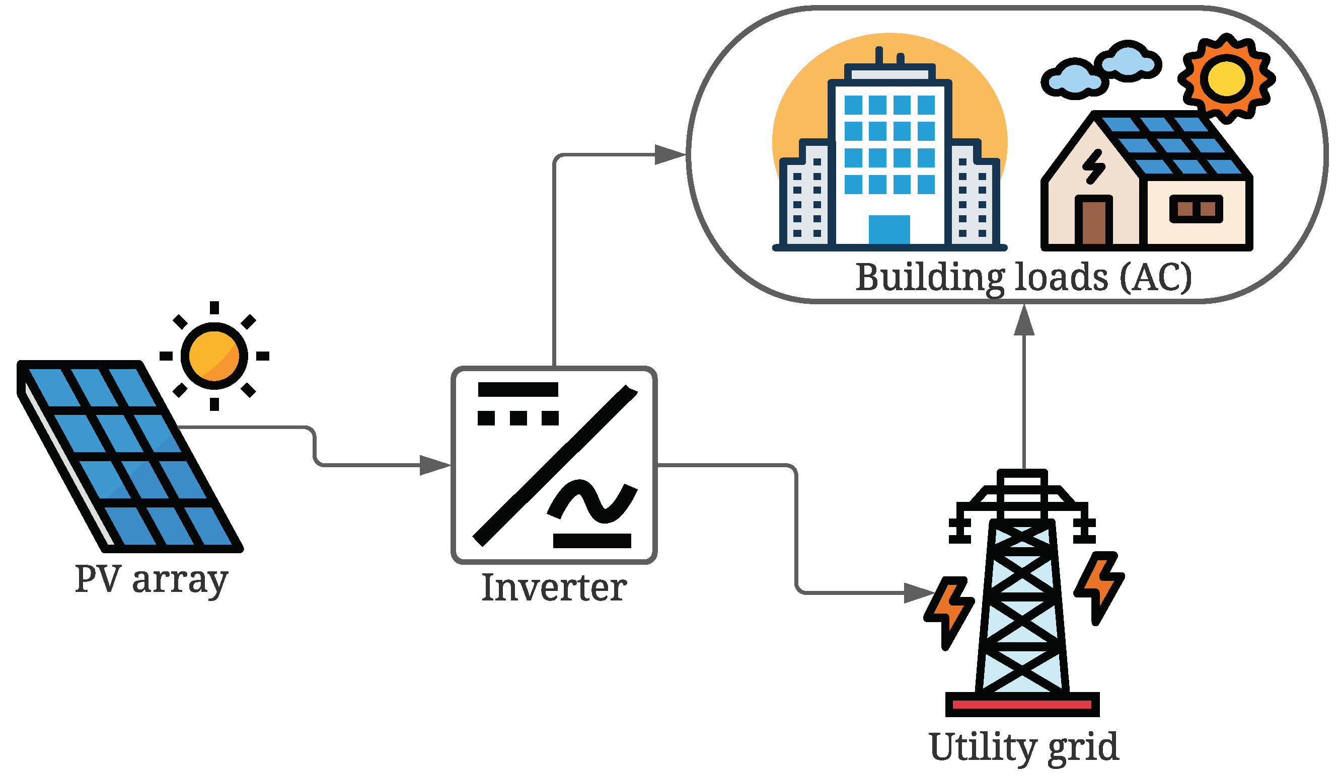
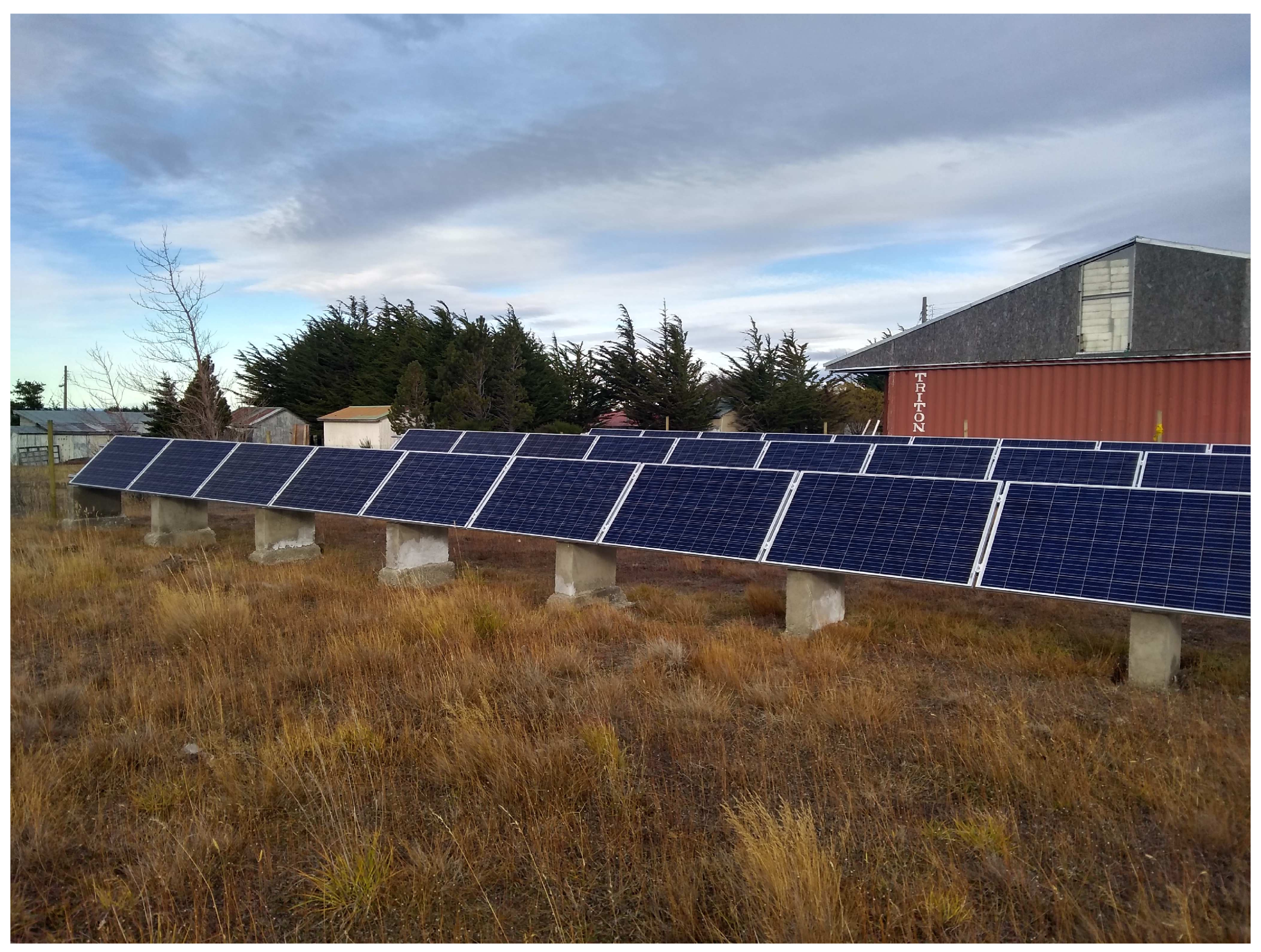
3.1. Description of the Grid-Connected Photovoltaic Architecture
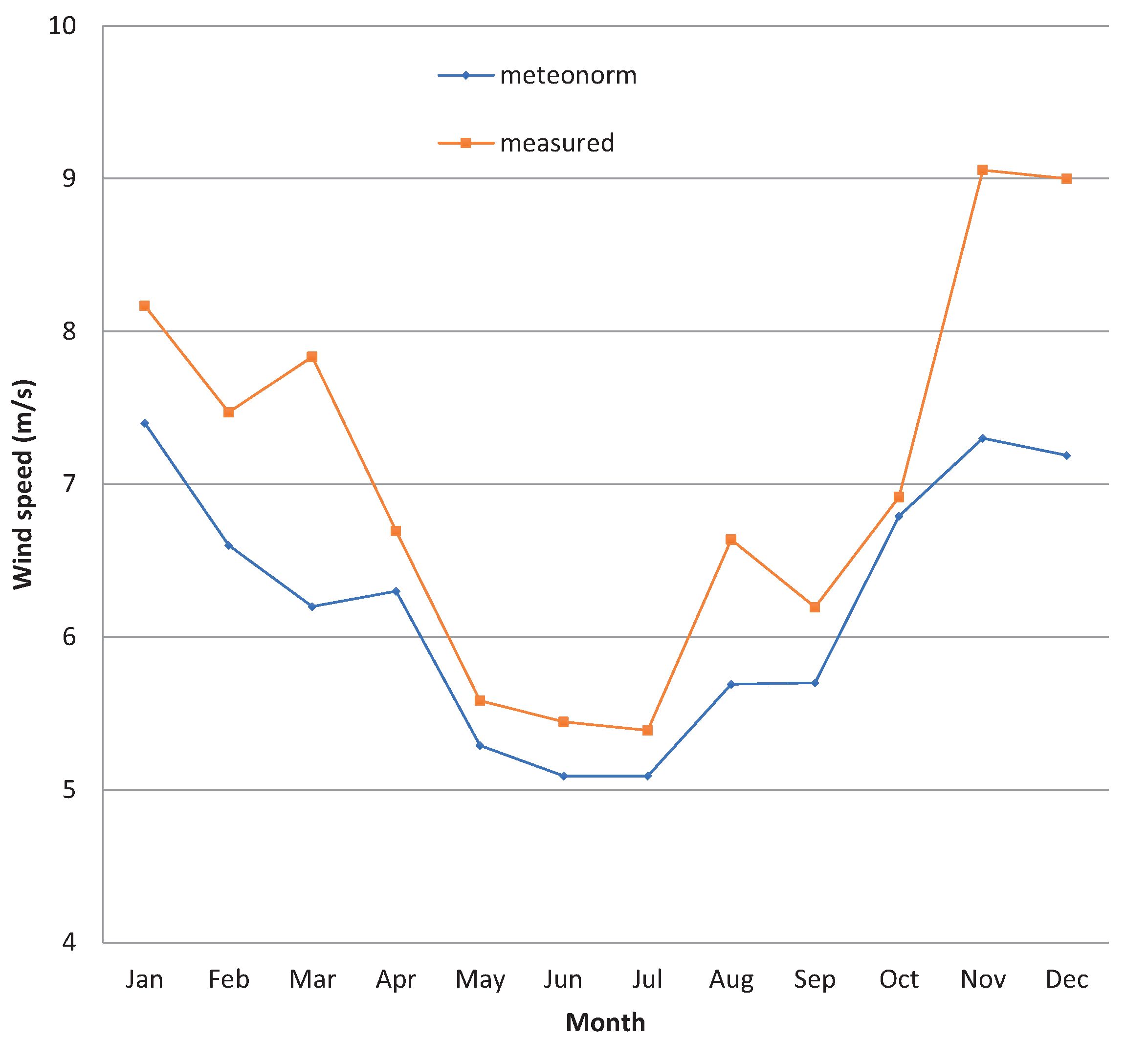
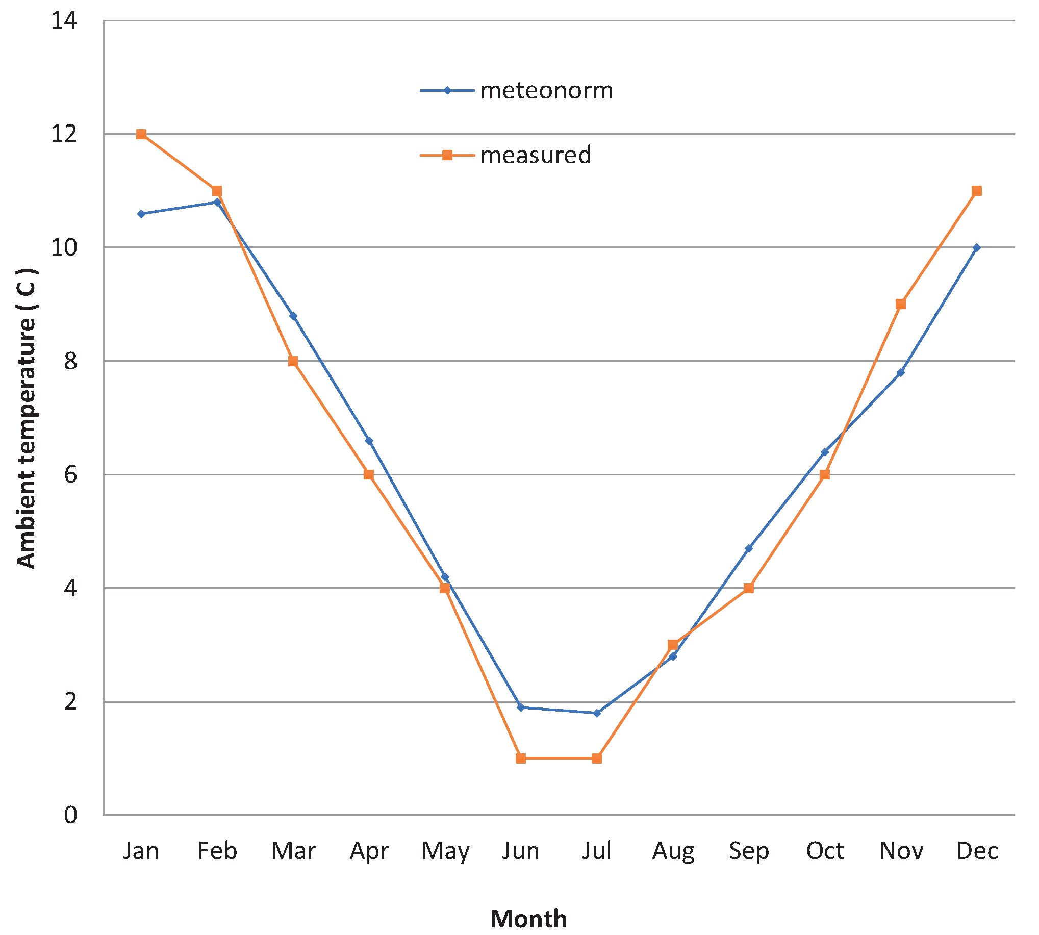
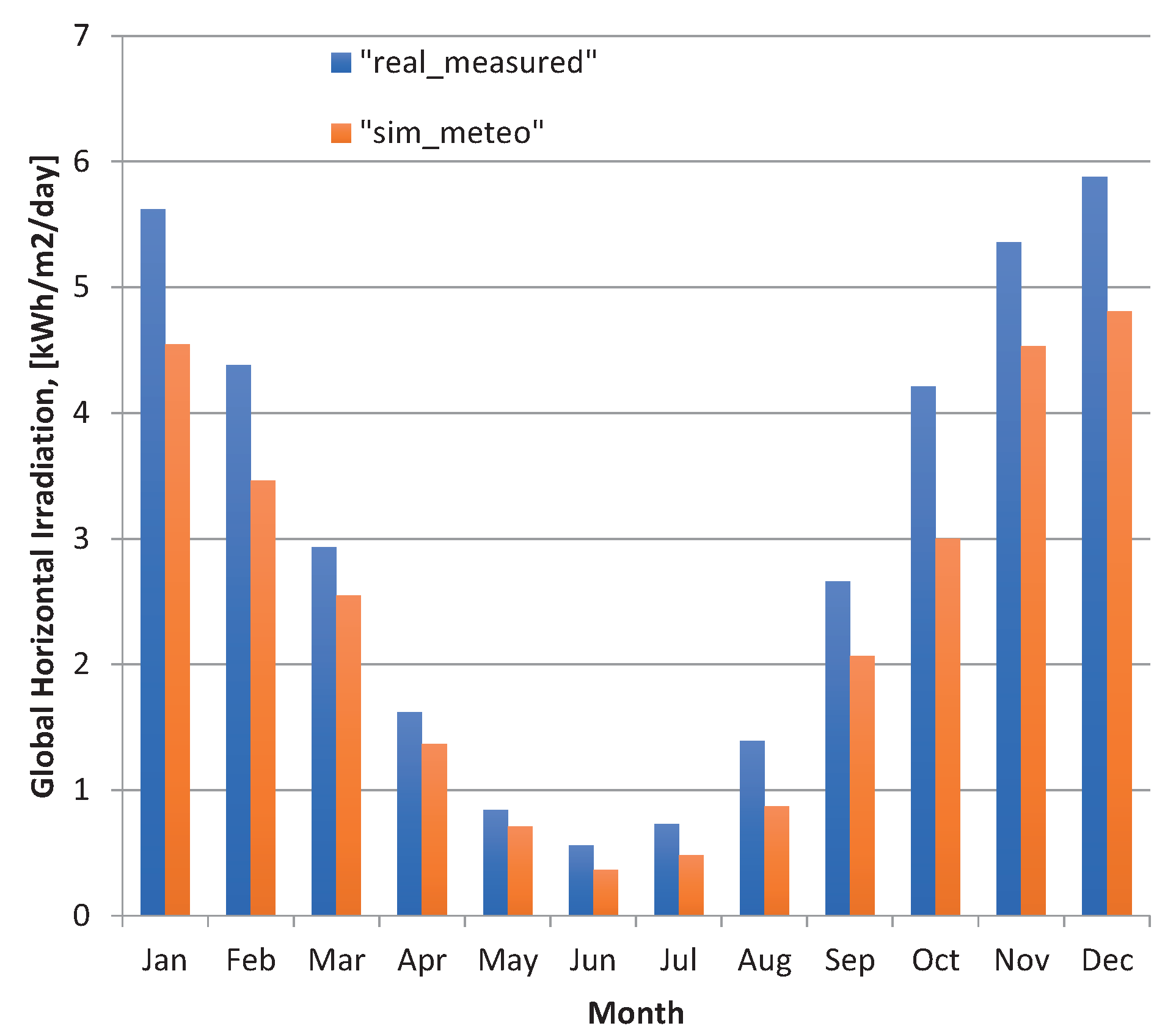
The key components of the system are shown in Figure 1, being the panels arrays, inverter and electricity utility meter. The panel array described in this work was installed using a system called solar panel racking on the ground with a “pitch” distance of 5 m, at the facilities of the public institution, Corporación Nacional Forestal (CONAF). The system shown in Figure 2, consisted of 31 polycrystalline PV panels (CS6P-265P). Each photovoltaic panel had a power rating of 265 Wp, with the technical characteristics shown in Table 1. The 31 PV panels were separated into three parallel strings: two strings with 10 panels connected in series and the other one with 11 series-connected panels, which were arranged facing north with a set tilt angle of 45° and azimuth angle of 0°.
The photovoltaic panels’ characteristics under normalised evaluation conditions were: AM1.5, irradiation of 1000 W/m 2 , panel temperature of 25 °C. A single inverter Fronius Symo 8.2-3-M with a rating of 8.2 kW and voltage operating range of 267–800 V was considered to convert DC voltages to AC voltages. The inverter had a DC input power rating of 8.2 kW and was connected to the grid by the fuse box and electrical grid meter. Since the array current and voltage were dependent on the prevailing weather characteristics, the inverter required adapting its operating point to work at the maximum efficiency. The technical descriptions of the photovoltaic system and inverter are detailed in Table 2.
Figure 3 shows a screenshot of the inverter display, with the voltage, frequency and current values of the PV system. The output of the inverter was connected to a Fronius Datamanager datalogger with WLAN and capabilities to record data at a logging interval of 5 min, the power to the grid being the most important channel to setup. The system was experimentally monitored in 2018.

3.2. Weather Data

In Punta Arenas City, only one ground station with available radiation data is located at the local airport, 35 km away from the project location. This situation, where no radiation measurement is available at the project location, has been one of the barriers to the deployment of photovoltaic projects in remote locations of the Magallanes region. In this work, two sources of weather data were used: measurements collected at Carlos Ibañez del Campo International Airport and the Meteonorm derived long-term data (1985–2005). The simulation outputs provide an insight into the validity of using long-term meteorological data instead of measured weather values (Figure 4). It shows a comparison between measurements collected in 2018 and the Meteonorm derived from long-term average wind speed values.
The Meteonorm wind speed information might not exactly match the values obtained for a specific month. However, it gives an illustrative figure because it consists of long-term statistical averaged data [26]. Clearly, the measured wind speed values were always over the Meteonorm data, as seen from Figure 4, and the prevailing wind direction in Punta Arenas is always northwest [2]. The consequence of the high wind speed can also be seen in the recorded environment temperatures, as shown in Figure 5. These are slightly lower than the Meteonorm values.
The measured average daily global horizontal solar irradiation per month (from the airport station) and the long-term average values derived from Meteonorm are shown in Figure 6. There are no pyranometers or reference cells at the project site, and thus, the incident irradiance is modelled. The nearest ground meteorological station is 35 km away. It can be seen that the measured data and monthly averaged Meteonorm derived daily solar irradiation show some deviations apart from the data for the months of May and June. This was expected since Meteonorm provides long-term monthly data for a determined site created from average statistical values over several years; thus, it will rarely be the same as the real values for any particular month.

3.3. PVSyst Simulation

PVSyst mainly requires meteorological data (global horizontal solar irradiation, wind speed and ambient temperature), as well as the electrical and mechanical specifications of the installed PV panels, the PV peak power, inverters’ data, position (tilt angle), orientation and available area as inputs. In this work, PVSyst received hourly weather data from two sources: measured and Meteonorm derived data such as solar irradiation, ambient temperature and wind speed at the PV project site. The technical specifications of the installed PV panels are shown in Table 1 and Table 2. The main design parameters of the simulation were orientation, panel, inverter, array to inverter matching and detailed losses.
The orientation, panel tilt and azimuth angle were defined, as well as the field type (fixed, tracking system, etc.). The panel and inverter type of the PV system were selected, and the number of sub-arrays and strings were chosen to match the inverter. Some of the loss parameters related to the PV system were wiring loss, ohmic losses, inverter behaviour, shading, panel quality, soiling loss factor and array incidence losses. These parameters were set according to system specifications, set at their default values or modified according to the experience from other similar projects. The main outputs of the simulation in a monthly basis were the produced energy (kWh/year), specific energy production (kWh/kWp/year), performance ratio and losses of the system.
The PVSyst simulation was based on the realization of hourly energy balances throughout a year. The calculation of energy yield in the grid-connected PV system includes three main steps: (a) the modelling of the incident irradiation in the plane-of-array, (b) the array direct current (DC) output and (c) the inverter alternating current (AC) output. For the first step, PVSyst offers two transposition approaches: the Hay and Perez models. The shading effect and the reflection losses at the surface of the modules are also calculated in order to finally obtain the effective incident irradiation reaching the panels’ surface. For Step (b), the electrical behaviour of the panels in the array was modelled using the “one-diode” equivalent circuit model in the case of crystalline silicon technologies. The in-operation module temperature used in the model was calculated as an energetic balance between the energy absorbed and the thermal losses from the panel to the surroundings. As a result, the DC power at the maximum power point (MPP) was calculated. In the last step, the AC output was calculated using the efficiency curve of the inverter. The final energy output was calculated after the corresponding losses due to AC cabling, and other losses were considered.

3.4. Performance and Loss Parameters: Description and Definition

To analyse the grid-connected PV architecture’s performance, the International Energy Agency (IEA) developed parameters indicated in [27] that have been used in various works [4,7,9,10,11,12,13,14,15,16,28]. These standard performance parameters give a pre-feasibility study of a photovoltaic system. In this work, reference yield Y R , final yield Y F , performance ratio P R , capacity factor C F and energy loss L were considered and calculated.
The reference yield Y R is the ratio of the total incident irradiation in panel H t (kWh/m 2 ) to the reference irradiation ( G o = 1 kW/m 2 ), and it is expressed as [29]:
Y R = H t G o
The final annual yield is the ratio of the total energy generated by the system and injected to the utility grid for a year and is given by the following expression [29]:
Y F , a = E A C , a P P V , r a t e d
where E A C , a (the PVSyst output called E G r i d ) is related to the total AC energy output (kWh) of the photovoltaic system per year (inverter terminal output) and P P V , r a t e d corresponds to the installed peak power of the photovoltaic array under rated conditions (STC). The final daily and monthly yields were calculated employing the ratio of the AC energy output (kWh) of the photovoltaic architecture to the nominal PV array peak power, respectively. The Y F parameter was used to compare with similar photovoltaic systems in other geographic regions.
The efficiency parameter P R corresponds to the ratio of energy supplied to the utility (final yield) to the nominal power indicated in the name plate of the photovoltaic panel at the rated characteristic (STC) of 1 kW/m 2 (reference yield). For most of the cases, P R values were larger in winter than during the summer months due to the elevated temperature of the PV module, an effect that generates additional losses. This value represents the amount of energy available after accounting for energy losses [15]. Usually, P R varies from 0.6 to 0.8 according to the site, solar irradiation and weather condition. This value is not related to the quantity of energy generated because a structure with a low value for P R in a high solar irradiation area could generate more energy in comparison to a system with a high value of P R operating in a location with low solar irradiation [28]. P R represents how close to the ideal performance a PV system is under real operating conditions and makes a comparison of photovoltaic systems possible, which is independent of the tilt angle, area, orientation and nominal capacity. The definition of the performance ratio is [29]:
P R = Y F Y R
Another performance parameter is the annual capacity factor C F . This parameter corresponds to the ratio between the current annual energy output and the energy that the photovoltaic system would produce if operated for 24 h at full rated power per day [29]:
C F = Y F , a 24 · 365 = P R · Y R 8760
C F depends on the PV system’s location where the higher the capacity factor, the better the performance of the PV system [9]. In addition to all the parameters mentioned above, loss parameters are also important in describing the performance of a photovoltaic system. The loss parameters can be classified into two types: system losses and array capture losses.
System losses: The inverter and the associated electrical components needed for the grid connection are factors that generate these losses [4]. The parameter is named L S and shows the difference among array yield Y a and final system yield Y F :
L S = Y a Y F
Array capture Losses: L C corresponds to the difference among reference yield Y R and array yield Y a , given by:
L C = Y R Y a
This magnitude of the losses in a PV array are due to several factors such as the PV cell temperature rise, dust accumulation, partial shading, errors in maximum power point tracking and mismatching [4].
The total loss of energy from this system L is found by taking the difference among reference yield Y R and final yield Y F :
L = L C + L S = Y R Y F
The above performance and losses parameters were compared experimentally and theoretically. Measured and Meteonorm derived climate datasets were both used for the simulations.

3.5. Thermal Losses of the PV Array

One of the major issues with PV systems is that the solar panels have moderately low efficiency levels (between 14 and 21%). That efficiency is particularly affected by the panel cells’ operating temperature. The temperature of the back of the module ( T B O M ) rising because of the incident irradiation can be obtained from an energy balance considering the ambient temperature and other parameters, included in the following expression [6]:
T B O M = α G ( 1 η ) U + T a m b
where G corresponds to the incident irradiation, α is the absorption of the PV panels, η is the panel efficiency and U is the thermal loss factor [6]:
U = U C + U v v
where parameter v corresponds to the wind velocity, parameter U c is related to the thermal loss constant and variable U v is the wind velocity constant. The values of the parameters of U c and U v of 20 W/m 2 K and 6 W/m 2 K/m/s were used in this study [6].
Equations (8) and (9) show the influence of the wind velocity on the back of the panel temperature ( T B O M ). A high wind velocity value leads to a decrease in the BOMtemperature. A decrease in the BOM temperature results in an increase in power production because of the lower values of the energy loss of the PV system, as mentioned in [15].

4. Results and Discussion

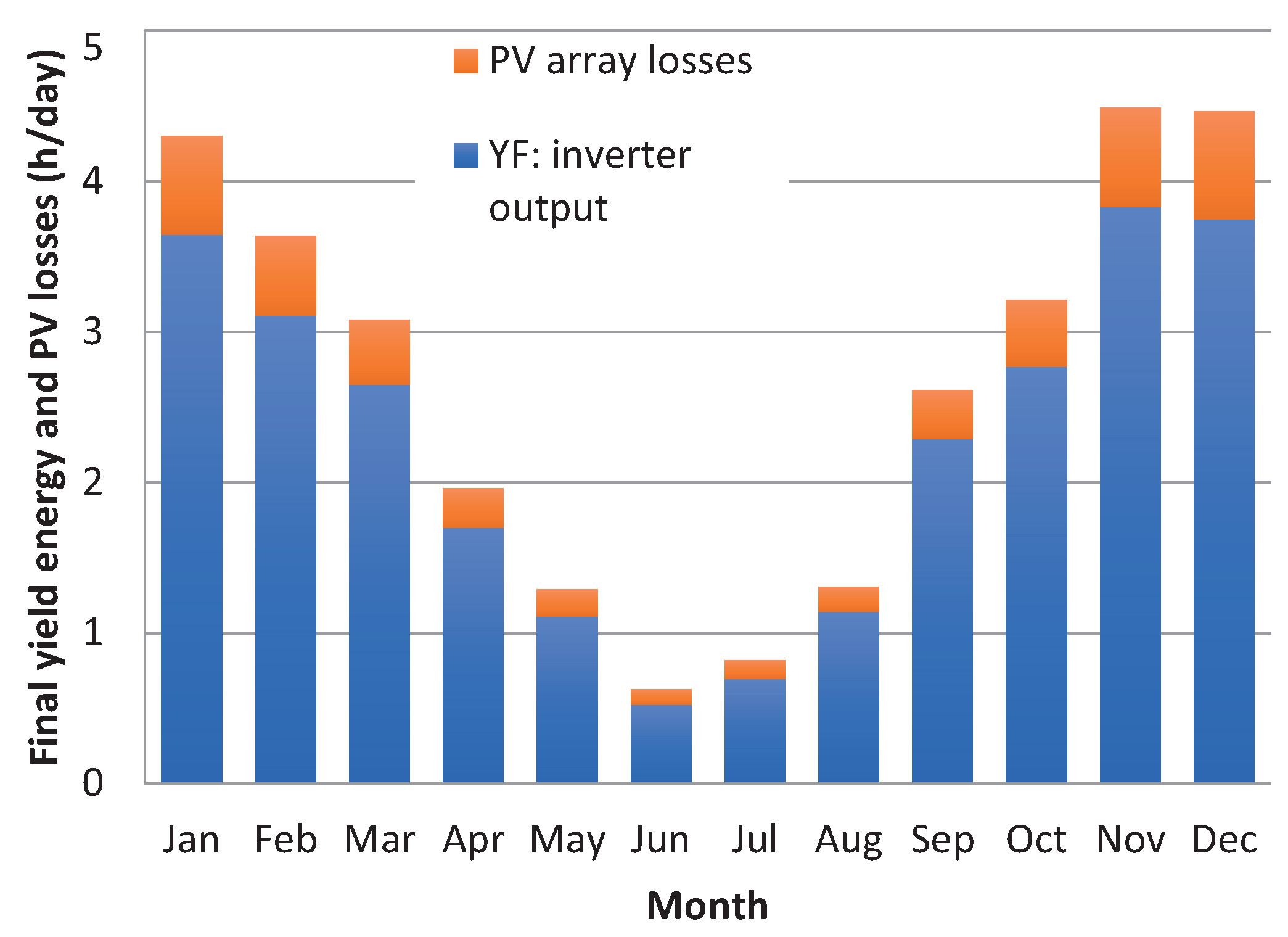
4.1. Annual Parameters Calculated

The three main annual data were obtained from the simulation results. The initial parameter was related to the total quantity of energy produced by the complete photovoltaic system, 6778.0 kWh/year. The second calculated parameter was given by the specific production per installed kWp equal to 825.6 kWh/kWp/year and a third parameter, P R = 85.5%, which is the average performance ratio per year, as shown in Table 4. On the other hand, a datalogger allowed the acquisition of energy injected into the grid coming from the inverter output terminal. Using these data and Equations (1)–(4), performance parameters Y R , Y F , P R and C F were calculated.

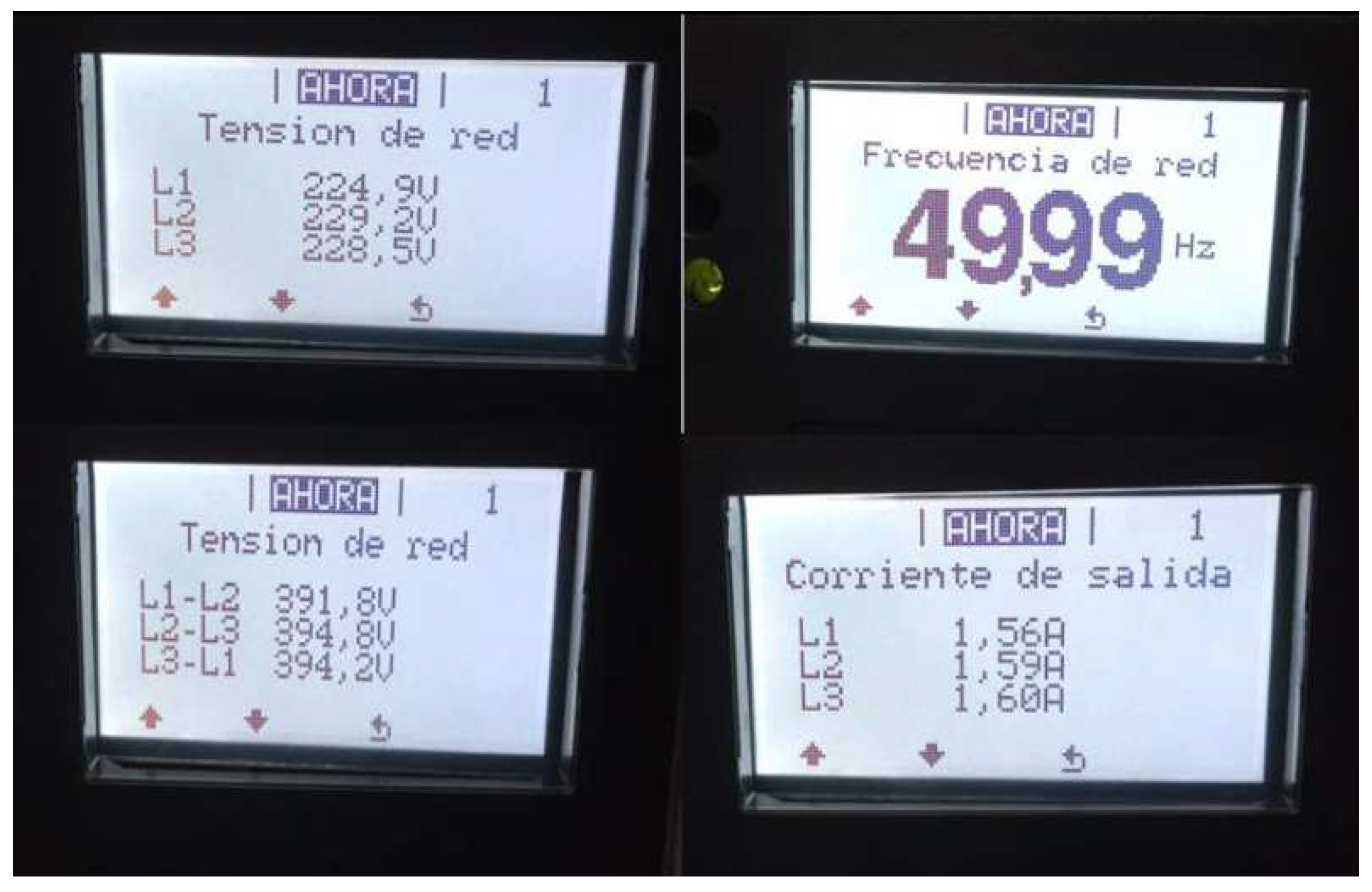
4.2. Main Results from PVSyst

In Table 3, ambient mean temperatures, the global irradiation on the horizontal plane and on the collector plane and effective global irradiation taking into account soiling losses and shading losses are shown. The energy generated by the PV array, as well as the energy injected into the grid including the losses in the electrical components and the PV array and the architecture’s efficiency were also calculated. The annually global irradiation on the horizontal plane is 873 kWh/m 2 , 965.1 kWh/m 2 for the global incident energy on an annual basis on the collector without optical corrections and 914.8 kWh/m 2 the effective global irradiation after optical losses, which were calculated for the particular location. With this irradiation, the annual DC energy generated from the photovoltaic array was 7005.3 kWh, and the annual AC energy injected into the grid was 6778.0 kWh, respectively. The annual mean efficiency of a photovoltaic array was 14.56%, and similarly, the annual average efficiency of the system was calculated as 14.08%. Plots comparing measured monthly/annual energy yield with simulated energy yield are shown in Figure 7. The measured final yield was 1318.51 kWh/kWp/year, while the simulated value was 825.60 kWh/kWp/year for the Meteonorm data, and the measured performance ratio was 89%, while the simulated value was 85.5% for the Meteonorm derived data, as can be seen in Table 4. The discrepancy between simulated and measured PV system output data may be due to several issues: an error in the system output data measurements, the design parameters used in the simulation that do not represent the real operating conditions of the system or using average meteorological data for the input (which is the case for Meteonorm) compared to using measurements from a nearby meteorological station. Figure 4 and Figure 6 show some differences for the local weather conditions for measured values versus the Meteonorm values, especially wind and solar irradiation data. This situation does not allows that PVSyst simulates the beneficial effects of high winds combined with better solar irradiation levels, finally underestimating the energy yield. The degraded module was defined during the simulation process. There is no tool in PVSyst for analysing this degradation explicitly. The user can create this degraded module by redefining the STC values I S C , V O C , I M P and V M P . The PV system was modelled in its first operation year 2018; thus, there is no possibility of any degradation. Because the system is in an open field area, the constant wind does not allow dust accumulation, so this factor was not considered. However, PVSyst allows the definition of soiling loss factors in monthly values. During the simulation, the soiling loss could be accounted for as an irradiance loss.

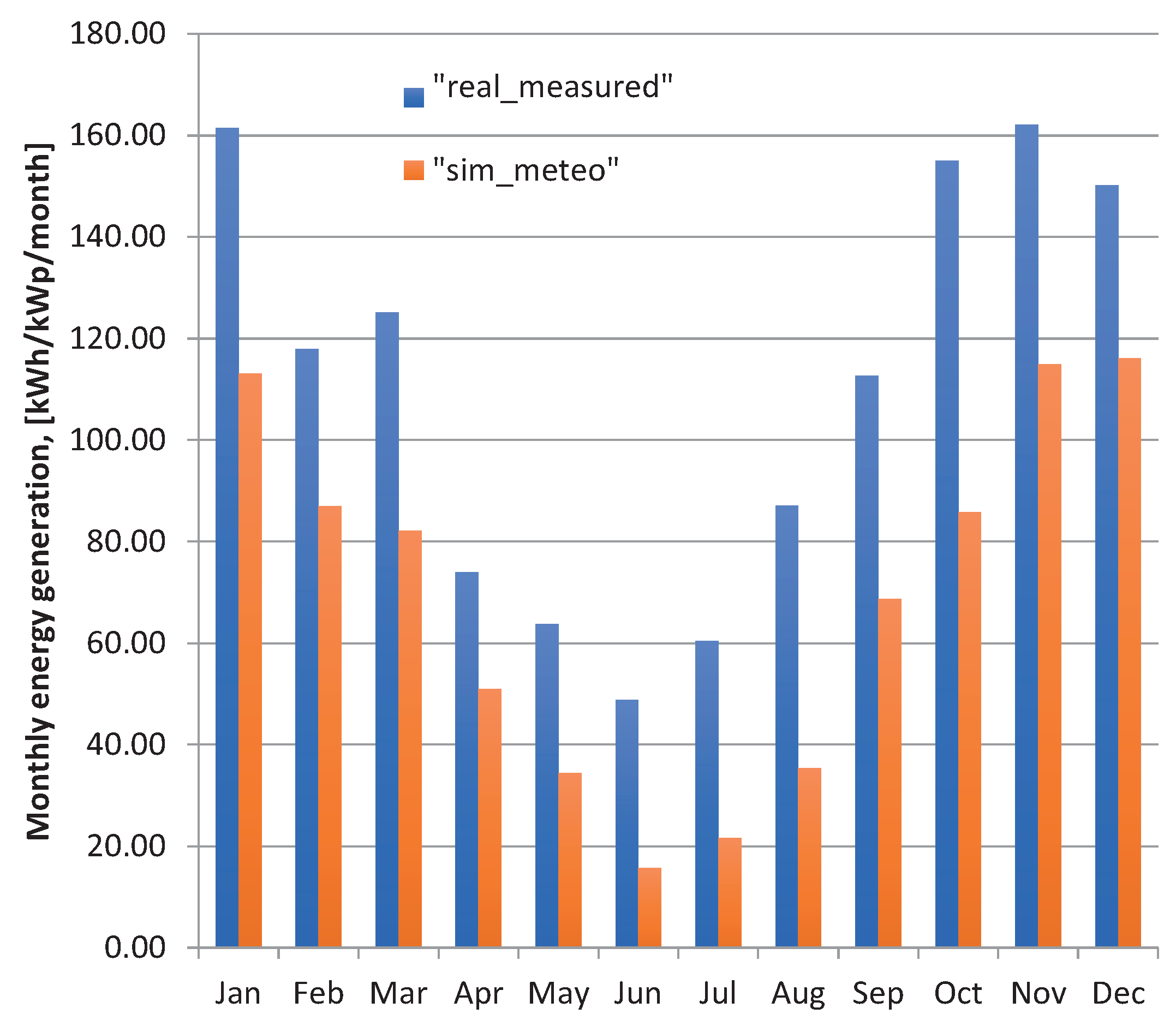
4.3. Normalised Energy Productions

As mentioned above, the normalised production is described by the IEC norm [27] and is the standardised parameter for the performance assessment of the PV system. This can be evaluated to compare the behaviour of photovoltaic architectures established in similar climatic conditions. Collection and system losses and useful produced energy per installed kWp/day were evaluated from the current simulation analysis and can be observed in Figure 8.
The collection losses of the PV array, named L c , were equal to 0.38 kWh/kWp/day. On the other hand, the produced useful energy, named Y F , from monthly averaged data varied between 0.52 and 3.83 kWh/kWp in June and November, respectively. When other months wee compared, the energy outputs from the months of April through September (winter season) were mostly low, especially in June. Some factors like the reduced number of sun hours and very low solar irradiation affected the useful produced energy. The daily final yield, named Y F , from yearly averaged data was 2.27 kWh/kWp.

4.4. Energy Injection of a Grid-Tied Solar PV System
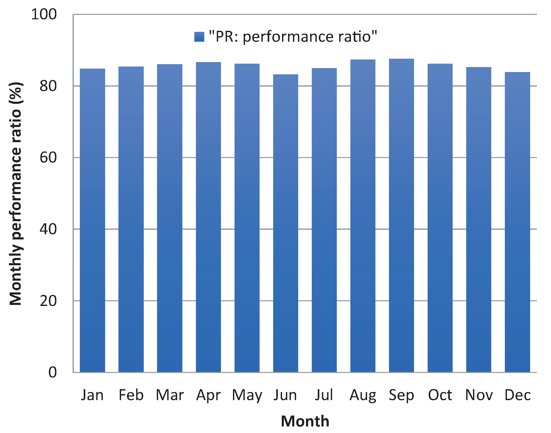
The energy introduced into the utility grid is different in relation to the energy generated by the photovoltaic array. The energy coming from the photovoltaic structure has to be transformed to AC power to be acceptable for integration into the electrical utility network. It is known that in the course of this process, some quantity of energy will be lost due to AC wiring loss. The 8.2 kWp PV system injects 6778 kWh to the grid on a yearly basis. The monthly specific electricity E A C - g r i d m injected into the grid is 825.60 kWh/kWp with an annual average daily final yield of 2.27 kWh/kWp, as shown in Table 4. The PV system generates and injects more energy to the electrical network in December, i.e., 953.4 kWh. The lowest amount injected to the grid is 128.5 kWh, which is in June. Detailed information about the injected energy to the grid is shown in Table 4.
Table 4. Performance ratio and injected energy into the electrical network using Meteonorm weather data (note: the kWp value is 8.2).
Month E AC - grid (kWh) E AC - grid m (kWh/kWp) E AC - grid d (kWh/kWp)Performance Ratio (%)
January928.1113.053.6584.8
February714.186.983.1185.4
March674.682.172.6586.0
April418.350.951.7086.6
May282.534.411.1186.2
June128.515.650.5283.3
July177.221.580.7085.0
August290.535.381.1487.4
September563.668.652.2987.6
October704.085.752.7786.2
November943.3114.903.8385.3
December953.4116.133.7583.9
Year6778.0825.602.2785.5
E A C - g r i d ” is the energy injected into the grid, “ E A C - g r i d m ” the monthly specific electricity produced and “ E A C - g r i d d ” the daily specific electricity produced.

4.5. Performance Ratio and Capacity Factor Results

The annual mean P R value for the 8.2 kWp PV system calculated from the simulated analysis was 85.5%. Figure 9 shows a small monthly variation in the value of P R on a monthly basis, and this can be seen in the monthly values included in Table 4. The highest P R value of 87.6 was obtained for the month of September. Furthermore, it can be appreciated that in the winter season (April to September), all P R values were likewise high. This seems to indicate that the simulated PV system approaches the ideal behaviour. In real working conditions, this might be mainly due to the module’s surface cooling by northwest cold winds, thus decreasing the ambient temperature and avoiding the module surface reaching a higher temperature.
The measured annual mean capacity factor C F obtained in this work was 15.1%, while the annual average capacity factor calculated from the simulation results with the Meteonorm derived long-term average values was 9.4%.

4.6. PV System Performance Parameters Compared with Other Installations

The normalised energy productions (kWh/kWp/day) allow potential comparisons among the different photovoltaic installations located in other geographical regions, because the effect of the system’s size is disregarded [9,15,30]. Table 5 shows performance parameters and other different characteristics of grid-tied photovoltaic systems. The measured annual mean daily final yield and the capacity factor of the photovoltaic architecture obtained in this work were 3.6 kWh/kWp/day and 15.1%, respectively, which are very close to those reported in Crete (Greece) and Eastern (India). In the present study, the photovoltaic architecture had a higher performance ratio and capacity factor in comparison to other systems, and moreover, it can be assessed that in Punta Arenas (lat. 53° S), the final yield improved over other cities with similar high latitudes such as Warsaw, Ballymena and Dublin (52°, 54° and 53° north), respectively.

5. Conclusions

An 8.2 kWp photovoltaic system connected to the electrical grid established in Punta Arenas (Chile) was simulated using the PVSyst software. The system also was experimentally monitored in 2018, and an evaluation and comparison of the monthly and annual performance of the system were carried out. From the simulation results, it can be concluded that the maximum energy fed into the grid was in December (953.4 kWh), and the least energy estimated at 128.5 kWh took place in the month of June. Moreover, on an annual basis, the annual energy supplied to the grid is 6778 kWh/year with specific production on an annual basis per installed kWp being 825.6 kWh/kWp/year. The final yield, capacity factor and annual performance ratio were 2.27 kWh/kWp, 9.4% and 85.5%, respectively. The purpose of the simulation was to establish a comparison between the measured and simulated results, and a difference was observed, showing more energy in the real installed PV system than the simulated photovoltaic model in PVSyst. The real results’ parameters could be used in a future work to calibrate those determined in the simulation. This will allow verifying if the increase in the real produced energy of the photovoltaic structure due to the lower working temperature of the solar cells was caused by northwest local winds. Despite low irradiation levels and low ambient temperature in Punta Arenas, the final yield per day Y F from the monitoring data was 3.6 kWh/kWp, a very good value when compared to other locations at high latitudes. Furthermore, a measured annual mean capacity factor C F obtained from this work of 15.1% and an annual performance ratio P R of 89% encourage greater use of photovoltaic technology to produce energy for the planned location in the Patagonia region. This paper demonstrates the energy production potential of a small-scale grid-connected photovoltaic system in the Magallanes region of Chile, an incentive for the use of photovoltaic energy in Patagonia. The presented results will inform policy markers, individuals and governmental organisations of this potential.

Author Contributions

All authors have contributed equally to the work. All authors read and agreed to the published version of the manuscript.

Funding

This work was supported by the Chilean Government under Seremi de Energía de Magallanes, Coorporación Nacional Forestal (Conaf), Project ANID/FONDECYT/1191028, ANID/FONDECYT/MEC80150056, FONDAP SERC Chile and Thematic Working Group on Energy, CUECH Research Network, Chile.

Conflicts of Interest

The authors declare no conflict of interest.

References

  1. MINENERGIA. Energía 2050: Política Energética Magallanes y Antártica Chilena; Technical Report; Ministerio de Energía: Punta Arenas, Chile, 2017. [Google Scholar]
  2. CERE-UMAG. Elaboración de Propuesta de Matriz Energética para Magallanes al 2050; Technical Report; Universidad de Magallanes: Punta Arenas, Chile, 2015. [Google Scholar]
  3. Pearsall, N. The Performance of Photovoltaic (PV) Systems: Modelling, Measurement and Assessment; Woodhead Publishing: Oxford, UK, 2016; Chapter 1; pp. 1–19. [Google Scholar]
  4. Kumar, N.M.; Kumar, M.R.; Rejoice, P.R.; Mathew, M. Performance analysis of 100 kWp grid connected Si-poly photovoltaic system using PVsyst simulation tool. Energy Procedia 2017, 117, 180–189. [Google Scholar] [CrossRef]
  5. Wijeratne, W.P.U.; Yang, R.J.; Too, E.; Wakefield, R. Design and development of distributed solar PV systems: Do the current tools work? Sustain. Cities Soc. 2018, 45, 553–578. [Google Scholar] [CrossRef]
  6. PVsyst Program. PV Syst User Manual. 2019. Available online: http://files.pvsyst.com/help/ (accessed on 7 May 2019).
  7. Omar, M.A.; Mahmoud, M.M. Grid connected PV-home systems in Palestine: A review on technical performance, effects and economic feasibility. Renew. Sustain. Energy Rev. 2018, 82, 2490–2497. [Google Scholar] [CrossRef]
  8. Adaramola, M.S. Techno-economic analysis of a 2.1 kW rooftop photovoltaic-grid-tied system based on actual performance. Energy Convers. Manag. 2015, 101, 85–93. [Google Scholar] [CrossRef]
  9. Sharma, R.; Goel, S. Performance analysis of a 11.2 kWp roof top grid-connected PV system in Eastern India. Energy Rep. 2017, 3, 76–84. [Google Scholar] [CrossRef]
  10. Milosavljević, D.D.; Pavlović, T.M.; Piršl, D.S. Performance analysis of a grid-connected solar PV plant in Niš, Republic of Serbia. Renew. Sustain. Energy Rev. 2015, 44, 423–435. [Google Scholar] [CrossRef]
  11. Baghdadi, I.; El Yaakoubi, A.; Attari, K.; Leemrani, Z.; Asselman, A. Performance investigation of a PV system connected to the grid. Procedia Manuf. 2018, 22, 667–674. [Google Scholar] [CrossRef]
  12. Allouhi, A.; Saadani, R.; Buker, M.; Kousksou, T.; Jamil, A.; Rahmoune, M. Energetic, economic and environmental (3E) analyses and LCOE estimation of three technologies of PV grid-connected systems under different climates. Sol. Energy 2019, 178, 25–36. [Google Scholar] [CrossRef]
  13. Allouhi, A.; Saadani, R.; Kousksou, T.; Saidur, R.; Jamil, A.; Rahmoune, M. Grid-connected PV systems installed on institutional buildings: Technology comparison, energy analysis and economic performance. Energy Build. 2016, 130, 188–201. [Google Scholar] [CrossRef]
  14. Tarigan, E.; Djuwari, D.; Kartikasari, F.D. Techno-economic simulation of a grid-connected PV system design as specifically applied to residential in Surabaya, Indonesia. Energy Procedia 2015, 65, 90–99. [Google Scholar] [CrossRef] [Green Version]
  15. Okello, D.; Van Dyk, E.; Vorster, F. Analysis of measured and simulated performance data of a 3.2 kWp grid-connected PV system in Port Elizabeth, South Africa. Energy Convers. Manag. 2015, 100, 10–15. [Google Scholar] [CrossRef]
  16. Elkholy, A.; Fahmy, F.; El-Ela, A.A.; Nafeh, A.E.S.A.; Spea, S. Experimental evaluation of 8 kW grid-connected photovoltaic system in Egypt. J. Electr. Syst. Inf. Technol. 2016, 3, 217–229. [Google Scholar] [CrossRef] [Green Version]
  17. Shukla, A.K.; Sudhakar, K.; Baredar, P. Simulation and performance analysis of 110 kWp grid-connected photovoltaic system for residential building in India: A comparative analysis of various PV technology. Energy Rep. 2016, 2, 82–88. [Google Scholar] [CrossRef] [Green Version]
  18. Watts, D.; Valdes, M.F.; Jara, D.; Watson, A. Potential residential PV development in Chile: The effect of net metering and net billing schemes for grid-connected PV systems. Renew. Sustain. Energy Rev. 2015, 41, 1037–1051. [Google Scholar] [CrossRef]
  19. Sahouane, N.; Dabou, R.; Ziane, A.; Neçaibia, A.; Bouraiou, A.; Rouabhia, A.; Mohammed, B. Energy and economic efficiency performance assessment of a 28 kWp photovoltaic grid-connected system under desertic weather conditions in Algerian Sahara. Renew. Energy 2019, 143, 1318–1330. [Google Scholar] [CrossRef]
  20. Zhang, W.; Pan, T.; Wu, D. A Novel Command-Filtered Adaptive Backstepping Control Strategy with Prescribed Performance for Photovoltaic Grid-Connected Systems. Sustainability 2020, 12, 7429. [Google Scholar] [CrossRef]
  21. Afzal, M.; Khan, M.; Hassan, M.; Wadood, A.; Uddin, W.; Hussain, S.; Rhee, S. A Comparative Study of Supercapacitor-Based STATCOM in a Grid-Connected Photovoltaic System for Regulating Power Quality Issues. Sustainability 2020, 12, 6781. [Google Scholar] [CrossRef]
  22. Gaisse, P.; Muñoz, J.; Villalón, A.; Aliaga, R. Improved Predictive Control for an Asymmetric Multilevel Converter for Photovoltaic Energy. Sustainability 2020, 12, 6204. [Google Scholar] [CrossRef]
  23. Mahmod Mohammad, A.; Mohd Radzi, M.; Azis, N.; Shafie, S.; Atiqi Mohd Zainuri, M. Novel Hybrid Approach for Maximizing the Extracted Photovoltaic Power under Complex Partial Shading Conditions. Sustainability 2020, 12, 5786. [Google Scholar] [CrossRef]
  24. Rezk, H.; Kanagaraj, N.; Al-Dhaifallah, M. Design and Sensitivity Analysis of Hybrid Photovoltaic-Fuel-Cell-Battery System to Supply a Small Community at Saudi NEOM City. Sustainability 2020, 12, 3341. [Google Scholar] [CrossRef] [Green Version]
  25. Kebede, A.; Berecibar, M.; Messagie, T.; Jemal, T.; Behabtu, H.; Van Mierlo, J. A Techno-Economic Optimization and Performance Assessment of a 10 kWp Photovoltaic Grid-Connected System. Sustainability 2020, 12, 7648. [Google Scholar] [CrossRef]
  26. METEONORM User Manuals, A.O. Available online: http://meteonorm.com/en/meteonorm-documents (accessed on 27 April 2019).
  27. Photovoltaic System Performance Monitoring-Guidelines for Measurement, Data Exchange and Analysis; Technical Committee GEL/82; BS EN 61724:1998; B.E. British Standards Institution: London, UK, 1998.
  28. Marion, B.; Kroposki, B.; Emery, K.; Del Cueto, J.; Myers, D.; Osterwald, C. Validation of a Photovoltaic Module Energy Ratings Procedure at NREL; Technical Report; National Renewable Energy Lab.: Golden, CO, USA, 1999. [Google Scholar]
  29. Congedo, P.; Malvoni, M.; Mele, M.; De Giorgi, M. Performance measurements of monocrystalline silicon PV modules in South-eastern Italy. Energy Convers. Manag. 2013, 68, 1–10. [Google Scholar] [CrossRef]
  30. Ayompe, L.; Duffy, A.; McCormack, S.; Conlon, M. Measured performance of a 1.72 kW rooftop grid connected photovoltaic system in Ireland. Energy Convers. Manag. 2011, 52, 816–825. [Google Scholar] [CrossRef] [Green Version]
  31. Kymakis, E.; Kalykakis, S.; Papazoglou, T.M. Performance analysis of a grid connected photovoltaic park on the island of Crete. Energy Convers. Manag. 2009, 50, 433–438. [Google Scholar] [CrossRef]
  32. Drif, M.; Pérez, P.; Aguilera, J.; Almonacid, G.; Gomez, P.; De la Casa, J.; Aguilar, J. Univer Project. A grid connected photovoltaic system of 200 kWp at Jaén University. Overview and performance analysis. Sol. Energy Mater. Sol. Cells 2007, 91, 670–683. [Google Scholar] [CrossRef]
  33. Mondol, J.D.; Yohanis, Y.; Smyth, M.; Norton, B. Long term performance analysis of a grid connected photovoltaic system in Northern Ireland. Energy Convers. Manag. 2006, 47, 2925–2947. [Google Scholar] [CrossRef]
  34. Pietruszko, S.; Gradzki, M. Performance of a grid connected small PV system in Poland. Appl. Energy 2003, 74, 177–184. [Google Scholar] [CrossRef]
  35. Sharma, V.; Chandel, S. Performance analysis of a 190 kWp grid interactive solar photovoltaic power plant in India. Energy 2013, 55, 476–485. [Google Scholar] [CrossRef]
  36. Adaramola, M.S.; Vågnes, E.E. Preliminary assessment of a small-scale rooftop PV-grid tied in Norwegian climatic conditions. Energy Convers. Manag. 2015, 90, 458–465. [Google Scholar] [CrossRef]
Figure 1. Layout of the grid-connected photovoltaic system [3].
Sustainability 12 09227 g001
Figure 2. Photo of the installed 8.2 kW grid-connected photovoltaic system in Punta Arenas.
Sustainability 12 09227 g002
Figure 3. Screenshots showing electrical parameters (voltage, current and frequency).
Sustainability 12 09227 g003
Figure 4. Average daily wind speed (m/s).
Sustainability 12 09227 g004
Figure 5. The daily ambient temperature in each month.
Sustainability 12 09227 g005
Figure 6. Monthly average daily horizontal solar irradiation.
Sustainability 12 09227 g006
Figure 7. The measured and simulated monthly energy yield.
Sustainability 12 09227 g007
Figure 8. Normalised energy productions per installed kWp and PV array losses.
Sustainability 12 09227 g008
Figure 9. Performance ratio.
Sustainability 12 09227 g009
Table 1. Characteristics of the photovoltaic panel.
PV PanelSpecification
TypePolycrystalline silicon
Nominal power ( P M A X ) 265 W P
Peak efficiency16.47%
Maximum power voltage ( V M P ) 30.6 V
Maximum power current ( I M P ) 8.66 A
Open circuit voltage ( V O C ) 37.7 V
Short circuit current ( I S C ) 9.23 A
Weight18 kg
Net (gross) panel surface1.6 m 2
Table 2. Technical information of the system.
PV ArraySpecification
Nominal power of the PV system8.2 W P
Number of panels31
Number of strings3
Number of modules for each string10 × 2 and 11 × 1
Number of inverters1
Net (gross) module area49.6 m 2
Grid-connected inverter
DC input side (PV array connection)
Maximum input voltage ( V D C m a x )1000 V
Rated input voltage267–800
AC output side (mains grid connection)
Output voltage (rated)220–400 V
Output current (rated)11.8 A
Output power (rated)8200 W
Grid frequency40–50 Hz
Power factor cos ϕ 0.85
Table 3. Results for the 8.2 kWp PV system (using Meteonorm weather data).
MonthGlobHor T amb GlobIncGlobEffEArrayE_GridEffArrREffSysR
(kWh/m 2 )(°C)(kWh/m 2 )(kWh/m 2 )(kWh)(kWh)(%)(%)
January141.09.70133.3126.0956.4928.114.3813.96
February97.08.40101.896.7736.5714.114.5114.07
March79.08.4095.590.9695.3674.614.6014.16
April41.06.7058.856.0433.2418.314.7814.27
May22.04.1039.937.7294.1282.514.8014.21
June11.02.1018.817.5136.8128.514.5613.67
July15.02.0025.423.8187.3177.214.7713.98
August27.02.8040.538.5303.3290.515.0214.38
September62.04.4078.474.8582.3563.614.8914.42
October93.06.2099.594.4726.5704.014.6514.19
November136.07.90134.7127.8970.8943.314.4514.04
December149.09.50138.4130.8982.7953.414.2413.82
Year873.06.00965.1914.87005.36778.014.5614.08
“GlobHor” is the Horizontal Global irradiation, “ T a m b ” the ambient Temperature, “GlobInc” the Global Incident irradiation in the collector plane, “GlobEff” the Effective Global correction for shadings, “EArray” the effective Energy at the output of the Array, “E_Grid the Energy injected into the Grid, “EffArrR” the Efficiency of the Array and “EffSysR” the Efficiency of the System.
Table 5. Performance parameters for different grid PV systems in the literature.
LocationPV TypeInstalledMonitoringFinal YieldCapacityPerformanceReference
Power (kWp)Period((kWh/kWp—Day)Factor (%)Ratio (%)
Crete, Greecepc-Si171.3620073.6615.367.4[31]
Jaén, Spainmc-Si2020032.7410.8465[32]
Ballymena, Northern Irelandmc-Si132001 to 20031.7–1.9-60–62[33]
Warsaw, Polanda-Si120012.279.4760–80[34]
Khatkar-Kalan, India 19020112.239.2774[35]
Punta Arenas, Chilepc-Si8.220183.615.189Present study
Dublin, Irelandmc-Si1.722008–20092.410.181.5[30]
As, Norwaypc-Si2.072013–20142.5510.683[36]
Nis, Serbiamc-Si2.02013–20143.1812.8893.6[10]
Eastern, Indiapc-Si11.22014–20153.6715.378[9]
Publisher’s Note: MDPI stays neutral with regard to jurisdictional claims in published maps and institutional affiliations.

