Abstract
This paper aims to examine the effects of economic policy uncertainty (measured by the World Uncertainty Index—WUI) on the level of CO2 emissions in the United States for the period from 1960 to 2016. For this purpose, we consider the unit root test with structural breaks and the autoregressive-distributed lag (ARDL) model. We find that the per capita income promotes CO2 emissions in the long run. Similarly, the WUI measures are positively associated with CO2 emissions in the long run. Energy prices negatively affect CO2 emissions both in the short run and the long run. Possible implications of climate change are also discussed.
1. Introduction
In today’s world, climate change is one of the leading problems which has the potential to harm sustainable economic performance both in developing and developed countries. The main reason for climate change is the atmospheric concentration of carbon dioxide and other greenhouse gases. These greenhouse gases lead to global warming, and global warming changes the climate around the globe. Therefore, it is essential to understand the driving factors of CO2 emissions. Our paper aims to examine the determinants of CO2 emissions, and special interest is given to the level of economic policy uncertainty, which is measured by the World Uncertainty Index (WUI) in [1].
CO2 emissions are strongly related to economic activities and the burning of fossil fuels [2]. Previous papers have indicated that there is a significant impact of income (which is usually measured by the per capita gross domestic product (GDP)) on environmental indicators [3]. However, income can decrease the level of environmental pollution in developed countries as the policymakers in these countries can consider health and other issues that can be more important than the level of per capita income or economic performance. Besides this, environmental pollution and greenhouse gases, which lead to global warming and climate change, threaten sustainable economic growth both in developed and developing economies.
A higher level of per capita income or economic growth will increase the level or the growth rate of CO2 emissions. However, policymakers should be more careful about CO2 emissions when per capita GDP increases. At this stage, policymakers can provide a more environment-friendly production process, and this structural transformation will reduce the growth rate of CO2 emissions. This view has been modeled as the Environmental Kuznets Curve (EKC) by [2,4]. The empirical results of [2,4] indicate that higher economic performance will cause an increase in the level of greenhouse gas emissions until a developing country experiences a specific level of per capita GDP. Then, greenhouse gas emissions will start to reduce. To put it differently, the EKC model suggests an inverted U-shaped impact of per capita GDP on the level of CO2 emissions [5].
On the other hand, along with the economic performance, energy usage can affect CO2 emissions. Specifically, higher energy consumption leads to a higher level of CO2 emissions. At this stage, previous papers have used different indicators of energy usage, and they have mostly considered the oil price to include the price effect in EKC modeling [3]. Different from previous papers, we use a broader and new measure of price effect and use the economy-wide energy price index in real prices in [6]. Therefore, we control for both the income effect and the price effect in the EKC modeling. These indicators should be significantly related to the level of CO2 emissions in the United States, which is one of the leading CO2 emitters in the world [7].
At this stage, we include the level of economic policy uncertainty (measured by the WUI) as a new driving factor of CO2 emissions in the United States. In other words, we extend the EKC model with the WUI and address a possible omitted variable bias. Indeed, researchers have indicated that uncertainty decreases investments [8,9,10,11] and leads to a decline in international trade [12]. However, the effects of uncertainty shocks on CO2 emissions seem to be neglected by empirical papers. We suggest that economic policy uncertainty can negatively or positively affect the level of CO2 emissions in an open economy. Our hypothesis is based on the fact that an open economy consists of the consumption of energy-intensive products and energy investments. At this stage, a higher level of WUI can cause a decline in the consumption of energy and pollution-intensive products; thus, CO2 emissions will be reduced as the WUI increases. We can label this effect the “consumption effect”.
On the other hand, a higher level of WUI can harm the investments in green energy and renewable energy projects; thus, CO2 emissions will be increased as the WUI increases. We can label this effect as the “investment effect (substitution effect)”. Naturally, the impact of the WUI on CO2 emissions depends on whether the “consumption effect” or the “investment effect” is dominant, where the latter is dominant in the case of the United States between 1960 and 2016. We suggest that economic policy uncertainty should be considered in EKC modeling, and it can provide important implications to sustain economic growth and to change the pattern of climate change via economic performance.
Overall, our study analyzes the determinants of CO2 emissions in the United States between 1960 and 2016. At this stage, we consider the WUI, which is introduced by [1]. Here, the authors of [1] measure the level of economic policy uncertainty in 143 developing and developed countries, and they show that this new uncertainty measure is negatively related to international trade and investments. At this juncture, the main objective of our study is to examine the impact of the WUI on CO2 emissions in the United States. Following previous papers on EKC modeling, we control for the income effect (which is measured by per capita GDP) and the price effect (which is measured by the novel index for real energy prices in [6] in modeling the level of CO2 emissions in the United States, i.e., the largest economy of the globe [13]. To the best of the authors’ knowledge, this paper is the first research in the empirical literature to examine the effects of the WUI on CO2 emissions following the EKC model. According to the empirical results, per capita income and economic policy uncertainty are positively related to CO2 emissions in the United States in the long run. Besides this, we observe that energy prices decrease the level of CO2 emissions in the United States both in the short run and the long run.
The rest of the paper is organized as follows. Section 2 provides a brief review of the literature for previous papers on the determinants of CO2 emissions in the United States. Section 3 describes the data and empirical models and explains the estimation procedure. Section 4 discusses the empirical results with possible implications. Section 5 is the concluding remarks.
2. Previous Papers on the Determinants of CO2 Emissions in the United States
There are various studies to examine the determinants of CO2 emissions in the United States. Along with the income effect and the price effect within the EKC model, various additional controls have been included. Financial development, foreign direct investment (FDI), trade openness, and urban population have been included as additional controls within the EKC model (see, e.g., [7]). At this stage, we review the papers which have used the time-series techniques and focus on only the case of the United States. For a detailed review of the related literature on other countries, one can refer to the recent study of [3]. We also review the papers, which focus on the aggregate level of CO2 emissions in the United States at the country level. Note that there are also several studies which focus on regional level data in the United States (see, e.g., [14,15]). Besides this, there are several papers which focus on sectoral level data in the United States (see, e.g., [16]).
In terms of these conditions, for example, the authors of [17] show that the income effect is not statistically significant. Still, the price effect significantly affects the level of CO2 emissions in the United States for the period from 1960 to 2000. Using the data for the period from 1960 to 2007, the authors of [18] also find that income is not a significant driver of CO2 emissions. While nuclear energy can significantly decrease CO2 emissions, renewable energy does not affect CO2 emissions in the United States. The authors of [7] use data for the period from 1960 to 2010 in the United States to examine the determinant factors of CO2 emissions. The authors find that energy consumption and urban population increase the level of CO2 emissions, while international trade decreases CO2 emissions. Financial development does not significantly affect environmental degradation. Income is also negatively related to CO2 emissions in the country. The authors of [19] also observe that the EKC model is not valid in the United States from 1980 through 2014. Besides this, renewable energy consumption reduces the level of CO2 emissions; however, non-renewable energy consumption increases environmental degradation. The authors of [20] investigate the validity of the EKC model in the United States by using data for the period from 1960 to 2016. The authors find that income, biomass energy consumption, and international trade decrease the level of CO2 emissions. Oil price does not have a significant impact on CO2 emissions in the country. The authors of [21] also show that energy consumption and foreign direct investments increase CO2 emissions in the United States. However, trade openness reduces CO2 emissions in the country.
The authors of [22] also state that the level of CO2 emissions in the United States declined by 12% between 2007 and 2016. The authors show that economic growth is negatively related to CO2 emissions. At this stage, improvements in energy efficiency, an increase in eco-friendly investments, and the rise of labor productivity are the main channels driving the negative impact of economic growth on CO2 emissions in the United States.
On the other hand, there are a few papers which investigate the impact of economic policy uncertainty on environmental indicators. For example, the authors of [16] use sectoral level data to examine the relationship between economic policy uncertainty and the growth rate of CO2 emissions in the United States. The authors find that the growth rate of CO2 emissions in the industrial, residential, and transportation sectors are significantly affected by economic policy uncertainty. However, the direction of the relationship is unclear. Besides this, the authors of [23] analyze the causal relationships among CO2 emissions, economic policy uncertainty, and energy consumption in the United Kingdom for the period from 1985 to 2017. The authors find that economic policy uncertainty decreases CO2 emissions in the short run, but there is no relationship in the long run. The authors of [24] use data from 1985 to 2017 in the United States to examine the effects of energy intensity on CO2 under economic policy uncertainty. The authors find that economic policy uncertainty promotes the detrimental impact of energy intensity on CO2 emissions.
Overall, various papers indicate that the validity of the income effect and the price effect is arguable, but we should include them into the estimations of the empirical model. There are also a few studies analyzing the effects of economic policy uncertainty on CO2 emissions. Still, there is no study which uses the WUI of [1] and the real energy price index of [6]. To the best of our knowledge, our paper provides the first evidence for the effects of the WUI on CO2 emissions in the empirical literature.
3. Data, Model, and Estimation Procedure
3.1. Data
We examine the drivers of CO2 emissions in the United States. The sample covers the annual data from 1960 to 2016. The start and the end dates of the empirical analysis are related to the availability of the data at the country level (note that energy price data at the global level can also be downloaded from https://ycharts.com/indicators/energy_index_world_bank#:~:text=Energy%20Price%20Index%20is%20at,30.71%25%20from%20one%20year%20ago). The dependent variable is the CO2 emissions (metric tons) per capita in logarithmic form (LnCO2_PC). The related data are obtained from [13]. We also use various explanatory variables. Specifically, GDP per capita (measured by the real 2010 USD prices) in logarithmic form (LnGDP_PC) captures the income impact in CO2 emission function. The data are collected from [13]. Energy prices (measured by the economy-wide index in real prices) in the logarithmic form (LnENPR) are also included in the model estimations. LnENPR captures the price impact in CO2 emission function, and the related data are obtained from the online appendix of [6].
Furthermore, we consider two measures of the World Uncertainty Indices (WUI_T2 and WUI_T6), and the data are obtained from [1]. We use the annual data, which are the averages of quarterly data. It is noteworthy that the authors of [1] introduce the WUI for 143 countries from the 1950s to 2020. The related indices are calculated by counting the frequency of the uncertainty (or its variant) in the Economist Intelligence Unit (EIU) country reports. The authors use the total number of words to normalize the WUI measures. A higher value of indices indicates a higher level of uncertainty. Refer to worlduncertaintyindex.com for details of the WUI measures. The measure of the WUI_t2 is the simple relative index in a given period. However, the measure of the WUI_t6 provides the three-quarter weighted moving average of the WUI. For example, 2019Q4 = (2019Q4 × 0.6) + (2019Q3 × 0.3) + (2019Q2 × 0.1)/3. Therefore, the WUI_t6 provides a more smoothed version of the WUI. According to [1], the WUI_t6 should be a benchmark measure for country-level analysis. We use both measures of the WUI to check the robustness of the empirical results for different measures of the WUI. Table 1 provides the descriptive statistics. Finally, we provide a correlation matrix in Table 2.

Table 1.
Descriptive statistics (1960–2016).
Table 2.
Correlation matrix (1960–2016).
The findings in Table 2 show that there is a negative correlation between the level of CO2 emissions and all explanatory variables. The correlation between the WUI and CO2 emissions is −0.49. Per capita income is positively correlated with energy prices (0.58) and the WUI measures (0.2). Besides this, the energy price index is also positively correlated with the WUI measures (0.13). These results indicate that there is no potential issue of multicollinearity among explanatory variables. There is a very high correlation between both measures of the WUI (0.97). Given that we separately use these two measures of the WUI, there will be no problem of multicollinearity. Finally, the quantile-quantile (Q-Q) graphs of the variables are illustrated in Figure 1.
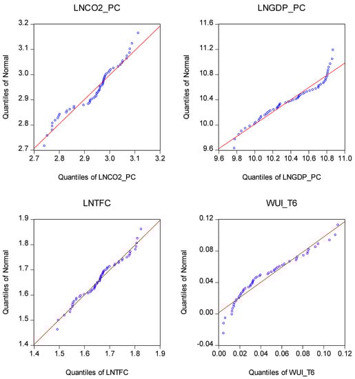
Figure 1.
Quantile-quantile (Q-Q) plots of the variables.
3.2. Empirical Model
We consider a well-known EKC model in the literature (e.g., [25,26]), and we aim to explain the drivers of per capita CO2 emissions. We include the per capita income, and energy prices are the main determinants of CO2 emissions. We also suggest that the WUI is a significant driver of CO2 emissions. At this stage, we can use the following function for an extended EKC model:
The function in Equation (1) can be written in model form, as such:
In Equations (1) and (2), is the per capita CO2 emissions, is the per capita income, is the index of energy prices, the World Uncertainty Index. Except for the WUI, the indicators are defined in logarithmic form. denotes an error term.
Following previous papers, we expect that > 0 and < 0. The EKC hypothesis demonstrates that > 0 since there should be a positive impact of income on CO2 emissions. Besides this, higher energy prices lead to lower CO2 emissions ( < 0).
Finally, the impact of economic policy uncertainty on CO2 emissions can be negative or positive. This evidence is due to the issue that an open economy consists of energy-intensive products and energy investments. Higher economic policy uncertainty can lead to a reduction in the consumption of energy and pollution-intensive products, and thus, CO2 emissions will be declined. This effect can be labeled as a “consumption effect” ( < 0). However, higher economic policy uncertainty can decrease the investments in green energy and renewable energy projects; thus, CO2 emissions will be increased. This effect can be labeled as an “investment effect” ( > 0). Naturally, the impact of economic policy uncertainty on CO2 emissions depends on whether the “consumption effect” or the “investment effect” is dominant. Surely, we must obtain a statistically significant coefficient of .
3.3. Estimation Procedure
First, we apply the unit root test of [27], which accounts for structural breaks in the level. Second, we utilize the bounds tests of [28] for the cointegration in the model with level term. We must reject the null hypothesis of “no cointegrating relationship in the time-series”. In other words, we should find a significant cointegration. Here, the critical values in [28,29] are considered, where the latter corrects small samples. Third, we estimate the short-run and the long-run coefficients in Equation (2) via the Autoregressive distributed lag (ARDL) model, introduced by [30]. Therefore, we estimate the following regression, where the per capita CO2 emissions are the dependent variable:
In Equation (3), Δ represents the first difference operator, denotes the error term, (i = 1, 2, 3, and 4) are the long-run parameters, and (i = 1, 2, 3, 4, and 5) are the short-run parameters in the ARDL model. Besides this, D2007 represents the dummy variable for structural breaks, which captures the period after 2007. The date is based on the findings of the unit root test of [27]. Following [31], we also report the following diagnostics of the ARDL estimations: Breusch–Godfrey serial correlation, Ramsey Reset model specification, Harvey heteroscedasticity tests as well as Cumulative Sum (CUSUM) and Cumulative Sum of Square (CUSUMSQ) tests for parameter stability.
We also utilize the long-run and the short-run Vector Error Correction (VEC) Granger Causality/Block Exogeneity Wald test. The following Equation contains the procedure of the related causality test:
In Equation (4), is the lagged error correction term, which represents the speed of adjustment to the long-run equilibrium. , , , and are random error terms, which are independent and identically distributed (i.i.d.).
4. Empirical Results and Discussion
4.1. Unit Root Test
First, we provide the results of the unit root test of [27], which are assumed a break on the level in Table 3.
Table 3.
Unit root test of [27].
According to the findings in Table 3, LnCO2PC, LnGDP_PC, LnENPR have a unit root, and their first differences are stationary. Therefore, these variables follow an I(1) process. On the other hand, the WUI_t2 and the WUI_t6 follow a stationary process; therefore, they follow the I(0) process. Since all variables do not follow an I(1) process, the traditional cointegration tests should not be considered. In light of these findings, we follow [32] and utilize the bounds cointegration test for cointegration and estimate ARDL model coefficients.
4.2. Bounds Test for Cointegration Analysis
We report the results of the bounds test for the model with the level in Table 4. We observe that the related F-statistics for the two models are higher than the critical values, which are provided by [28,29]. As a result, the null hypothesis (there is no level cointegration) is rejected. We observe the significant cointegration relationship among the related indicators.
Table 4.
Bounds tests for cointegration analysis.
4.3. Long-Run Estimates of the ARDL Model
Then, we estimate the long-run coefficients of the ARDL model, and the results are reported in Table 5. Initially, the ARDL model has suitable misspecification and stable parameters, and there are no problems in terms of serial correlation and heteroscedasticity. Specifically, the Breusch–Godfrey test shows that there is no serial correlation problem in residuals. The Ramsey Reset test indicates that there is no misspecification problem in the model. According to the results of the Harvey Heteroskedasticity test, the variances of the models are homoscedastic. Finally, CUSUM and CUSUMSQ tests show that the coefficients of regressions are stable over time, and possible structural breaks are correctly modeled.
Table 5.
Long-run coefficients of the Autoregressive Distributed Lag (ARDL) model estimations.
According to the results in Table 5, the lagged dependent variables are statistically significant up to three lags (LnCO2PCt−1, LnCO2PCt−2, and LnCO2PCt−3). Coefficients, which represent the structural break (dummy variable for the period after 2007), are statistically insignificant. The long-run income impact, which is measured by log current per capita GDP (LnGDP_PC t), is found as inelastic and positive (0.64 for the first model and 0.59 for the second model). Following this evidence, we can conclude that income promotes CO2 emissions. The long-run price impact, which is captured by the index of real energy price (LnENPR t), is also inelastic but negative (−0.069 for the first model and −0.081 for the second model). This evidence indicates that energy prices decrease CO2 emissions in the long run.
Finally, the long-run impact of economic policy uncertainty, which is measured by the indices of the WUI_t2 and the WUI_t6, is found as elastic. Note that the current WUI measures have negative coefficients, but they are statistically insignificant. The lagged WUI measures positively affect CO2 emissions, and the coefficients are elastic (0.063 for the first model and 0.171 for the second model). This evidence implies that higher economic policy uncertainty in the previous year in the United States leads to higher CO2 emissions in the current year.
4.4. Short-Run Estimates of the ARDL Model
We also provide the findings of the short-run coefficients for the ARDL model estimations in Table 6. Note that the coefficient of the Error Correction Term (ECTt−1) in the lagged form is obtained as −0.026 (p < 0.01) and −0.016 (p < 0.01) for the first model and the second model, respectively. This evidence implies that the level of CO2 emissions in the United States converges in the long-run equilibrium by a low-level speed of adjustment ([32]), via the channels of per capita income, energy price, and economic policy uncertainty.
Table 6.
Short-run coefficients of the ARDL model estimates.
The findings in Table 6 show that the lagged dependent variables are statistically insignificant up to two lags (∆LnCO2PCt−1 and ∆LnCO2PCt−2). Coefficients of the structural breaks are also statistically insignificant. The short-run income impact, which is measured by ∆LnGDP_PCt, is obtained as inelastic and positive (0.64 for the first model and 0.59 for the second model). Therefore, income also increases CO2 emissions in the short run. The short-run price impact, which is measured by ∆LnENPRt, is also inelastic and negative (−0.072 for the first model and −0.062 for the second model). This evidence means that energy prices also reduce CO2 emissions in the short run. Finally, the short-run impact of economic policy uncertainty, which is measured by the indices of the WUI_t2 and the WUI_t6, is found as negative but statistically insignificant. This evidence shows that economic policy does not significantly affect CO2 emissions in the United States in the short run.
4.5. VEC Granger Causality
We also provide the findings of the long-run and the short-run VEC Granger Causality/Block Exogeneity Wald test in Table 7. The findings indicate that the long-run causality for both models of CO2 emissions is statistically significant (p < 0.01). This evidence is in line with the results of long-run ARDL model estimates.
Table 7.
VEC Granger Causality/Block Exogeneity Wald Tests.
In terms of short-run causality, only the energy prices cause CO2 emissions in the United States. The income and economic policy uncertainty measures do not significantly cause CO2 emissions in the short run. Therefore, the results for the income coefficient in the short-run ARDL model estimates are not robust enough to run a different econometric method. Overall, income and economic policy uncertainty increase CO2 emissions only in the long run, while energy prices are negatively related to CO2 emissions both in the short run and the long run.
4.6. Discussion of Results and Potential Implications
Our results show that there is a positive impact of income on CO2 emissions in the long run. This evidence implies that our extended EKC-based model is valid in the United States in the long run. However, short-run income (economic growth) does not affect environmental pollution, and this evidence should be expected in developed countries, such as the United States. Besides this, energy prices yield lower CO2 emissions in the United States both in the short run and the long run, as it is expected. It seems that energy prices are only the determinant of CO2 emissions in the United States both in the short run and the long run. This issue also means that the future levels of CO2 emissions in the United States can be predicted from its previous levels as well as from per capita income, energy prices, and economic policy uncertainty measures.
We also find that economic policy uncertainty measures are positively related to CO2 emissions in the United States in the long run. We can suggest that decreasing the level of economic policy uncertainty can promote a more environment-friendly transformation process in the United States, i.e., the structural transformation from fossil-fuel energy to renewable energy in the production. At this stage, the COVID-19 pandemic is creating a remarkable rise in uncertainty in economic policies in the United States. Our results also indicate that this issue can make the climate change problem worse. Overall, stable and transparent economic policies can help to mitigate the level of CO2 emissions in the United States in the long run, and this is our novel contribution to the existing empirical literature. Note that our findings are obtained by the whole CO2 emissions in the United States, and this issue is the limitation of our study. Of course, we should enhance our knowledge of the level of CO2 emissions for each sector in the United States to understand better how economic policy uncertainty affects environmental pollution in the country.
5. Concluding Remarks
In this paper, we investigate the effects of economic policy uncertainty, which is measured by the WUI of [1] on CO2 emissions in the United States over the period from 1960 to 2016. We extended the EKC approach by incorporating the WUI. For this purpose, we initially run the unit root test of [27] with structural breaks and then the bounds cointegration analysis. Following the results of the initial tests, we estimate the ARDL model of [30]. We also utilize the VEC Granger Causality test to check the robustness of the short-run and the long-run coefficients. To the best of the authors’ knowledge, this paper is the first research to examine the effects of the WUI on CO2 emissions.
The empirical results are as follows. First, the per capita income increases CO2 emissions in the long run. Second, the index of energy prices decreases the level of CO2 emissions both in the short run and in the long run. Third, the WUI indices are positively associated with CO2 emissions in the long run, and this finding is the novel evidence of the existing environmental economics literature.
Future papers for investigating the effects of economic policy uncertainty on CO2 emissions can focus on other large economies, such as Brazil, China, and India. Finally, our paper uses the novel index of energy prices of [6] at the aggregated level. At this stage, future studies can use different types of energy prices (e.g., coal or oil prices) in developing or developed countries.
Author Contributions
Conceptualization, Q.W., and K.X.; methodology, Z.L.; software, Q.W.; validation, K.X., Q.W., and Z.L.; formal analysis, Q.W.; investigation, K.X.; resources, K.X.; data curation, Z.L.; writing—original draft preparation, Q.W.; writing—review and editing, K.X.; visualization, K.X.; supervision, Z.L.; project administration, Z.L. All authors have read and agreed to the published version of the manuscript.
Funding
The authors acknowledge the financial supports from the Philosophy & Social Science Fund of Tianjin City, China (“Prompting the Market Power of Tianjin City’s E-commerce Firms in Belt & Road Countries: A Home Market Effect Approach).
Conflicts of Interest
The authors declare no conflict of interest.
References
- Ahir, H.; Bloom, N.; Furceri, D. The World Uncertainty Index; Policy Research (SIEPR) Working Paper; No. 19-027; Stanford Institute for Economic, Stanford University: Stanford, CA, USA, 2019. [Google Scholar]
- Grossman, G.M.; Krueger, A.B. Economic Growth and the Environment. Q. J. Econ. 1995, 110, 353–377. [Google Scholar] [CrossRef]
- Shahbaz, M.; Sinha, A. Environmental Kuznets Curve for CO2 Emissions: A Literature Survey. J. Econ. Stud. 2019, 46, 106–168. [Google Scholar] [CrossRef]
- Grossman, G.M.; Krueger, A.B. Environmental Impacts of a North American Free Trade Agreement; National Bureau of Economic Research (NBER) Working Paper; No. 3914; NBER: Cambridge, MA, USA, 1991. [Google Scholar]
- Dinda, S. Environmental Kuznets Curve Hypothesis: A Survey. Ecol. Econ. 2004, 49, 431–455. [Google Scholar] [CrossRef]
- Liddle, B.; Huntington, H. Revisiting the Income Elasticity of Energy Consumption: A Heterogeneous, Common Factor, Dynamic OECD & Non-OECD Country Panel Analysis. Energy J. 2020, 41, 207–229. [Google Scholar]
- Dogan, E.; Turkekul, B. CO2 Emissions, Real Output, Energy Consumption, Trade, Urbanization and Financial Development: Testing the EKC Hypothesis for the USA. Environ. Sci. Pollut. Res. 2016, 23, 1203–1213. [Google Scholar] [CrossRef] [PubMed]
- Bernanke, B.S. Irreversibility, Uncertainty, and Cyclical Investment. Q. J. Econ. 1983, 98, 85–106. [Google Scholar] [CrossRef]
- Bloom, N. The Impact of Uncertainty Shocks. Econometrica 2009, 77, 623–685. [Google Scholar]
- Dixit, A.K.; Dixit, R.K.; Pindyck, R.S. Investment under Uncertainty; Princeton University Press: Princeton, NJ, USA, 1994. [Google Scholar]
- Rodrik, D. Policy Uncertainty and Private Investment in Developing Countries. J. Dev. Econ. 1991, 36, 229–242. [Google Scholar] [CrossRef]
- Novy, D.; Taylor, A.M. Trade and Uncertainty. Rev. Econ. Stat. 2020, 102, 749–765. [Google Scholar] [CrossRef]
- World Bank. The World Development Indicators; The World Bank: Washington, DC, USA, 2020. [Google Scholar]
- Roach, T. A Dynamic State-level Analysis of Carbon Dioxide Emissions in the United States. Energy Policy 2013, 59, 931–937. [Google Scholar] [CrossRef]
- Tzeremes, P. Time-varying Causality between Energy Consumption, CO2 Emissions, and Economic Growth: Evidence from US States. Environ. Sci. Pollut. Res. 2018, 25, 6044–6060. [Google Scholar] [CrossRef] [PubMed]
- Jiang, Y.; Zhou, Z.; Liu, C. Does Economic Policy Uncertainty Matter for Carbon Emission? Evidence from US Sector Level Data. Environ. Sci. Pollut. Res. 2019, 26, 24380–24394. [Google Scholar] [CrossRef]
- Soytas, U.; Sari, R.; Ewing, B.T. Energy Consumption, Income, and Carbon Emissions in the United States. Ecol. Econ. 2007, 62, 482–489. [Google Scholar] [CrossRef]
- Menyah, K.; Wolde-Rufael, Y. CO2 Emissions, Nuclear Energy, Renewable Energy, and Economic Growth in the US. Energy Policy 2010, 38, 2911–2915. [Google Scholar] [CrossRef]
- Dogan, E.; Ozturk, I. The Influence of Renewable and Non-renewable Energy Consumption and Real Income on CO2 Emissions in the USA: Evidence from Structural Break Tests. Environ. Sci. Pollut. Res. 2017, 24, 10846–10854. [Google Scholar] [CrossRef] [PubMed]
- Shahbaz, M.; Solarin, S.A.; Hammoudeh, S.; Shahzad, S.J.H. Bounds Testing Approach to Analyzing the Environment Kuznets Curve Hypothesis with Structural Breaks: The Role of Biomass Energy Consumption in the United States. Energy Econ. 2017, 68, 548–565. [Google Scholar] [CrossRef]
- Shahbaz, M.; Gozgor, G.; Adom, P.K.; Hammoudeh, S. The Technical Decomposition of Carbon Emissions and the Concerns about FDI and Trade Openness Effects in the United States. Int. Econ. 2019, 159, 56–73. [Google Scholar] [CrossRef]
- Wang, Q.; Jiang, X.T.; Ge, S.; Jiang, R. Is Economic Growth Compatible with a Reduction in CO2 Emissions? Empirical Analysis of the United States. Resour. Conserv. Recycl. 2019, 151, 104443. [Google Scholar] [CrossRef]
- Adedoyin, F.F.; Zakari, A. Energy Consumption, Economic Expansion, and CO2 Emission in the UK: The Role of Economic Policy Uncertainty. Sci. Total Environ. 2020, 738, 140014. [Google Scholar] [CrossRef]
- Ulucak, R.; Khan, S.U.D. Relationship between Energy Intensity and CO2 Emissions: Does Economic Policy Matter? Sustain. Dev. 2020, 28, 1457–1464. [Google Scholar]
- Narayan, P.K.; Saboori, B.; Soleymani, A. Economic Growth and Carbon Emissions. Econ. Model. 2016, 53, 388–397. [Google Scholar] [CrossRef]
- Peng, H.; Tan, X.; Li, Y.; Hu, L. Economic Growth, Foreign Direct Investment and CO2 Emissions in China: A Panel Granger Causality Analysis. Sustainability 2016, 8, 233. [Google Scholar] [CrossRef]
- Perron, P. Further Evidence on Breaking Trend Functions in Macroeconomic Variables. J. Econom. 1997, 80, 355–385. [Google Scholar] [CrossRef]
- Pesaran, M.H.; Shin, Y.; Smith, R.J. Bounds Testing Approaches to the Analysis of Level Relationships. J. Appl. Econom. 2001, 16, 289–326. [Google Scholar] [CrossRef]
- Narayan, P.K. The Saving and Investment Nexus for China: Evidence from Cointegration Tests. Appl. Econ. 2005, 37, 1979–1990. [Google Scholar] [CrossRef]
- Pesaran, M.H.; Shin, Y. An Autoregressive Distributed Lag Modelling Approach to Cointegration Analysis. In Econometrics and Economic Theory in the 20th Century; Strom, S., Ed.; The Ragnar Frisch Centennial Symposium: Cambridge, UK, 1999; pp. 371–413. [Google Scholar]
- Gozgor, G.; Can, M. Does Export Product Quality Matter for CO2 Emissions? Evidence from China. Environ. Sci. Pollut. Res. 2017, 24, 2866–2875. [Google Scholar] [CrossRef]
- Narayan, P.K.; Smyth, R. What Determines Migration Flows from Low-Income to High-Income Countries? An Empirical Investigation of Fiji-U.S. Migration 1972–2001. Contemp. Econ. Policy 2006, 24, 332–342. [Google Scholar] [CrossRef]

Publisher’s Note: MDPI stays neutral with regard to jurisdictional claims in published maps and institutional affiliations. |
© 2020 by the authors. Licensee MDPI, Basel, Switzerland. This article is an open access article distributed under the terms and conditions of the Creative Commons Attribution (CC BY) license (http://creativecommons.org/licenses/by/4.0/).