Importance of Proper Monetary Liquidity: Sustainable Development of the Housing and Stock Markets

Abstract

In this paper, we infer that when no excess monetary liquidity exists, people tend to invest available capital in assets associated with a high return or low risk. However, when excess monetary liquidity occurs, capital may successively boost asset markets, and the stock market wealth is thus likely to spill into housing markets, resulting in bubbles in these two markets and therefore in the unsustainable development of both the housing and stock markets. This paper uses relevant data from the United Kingdom from January 1991 to March 2020 to verify whether excess monetary liquidity is a crucial factor determining the relationship between the housing and stock markets. Continuous and structural changes are found to exist between housing price and stock price returns. This paper employs the time-varying coefficient method for estimation and determines that the influence of stock price returns on housing returns is dynamic, and an asymmetrical effect can occur according to whether excess monetary liquidity exists. An excessively loose monetary policy increases asset prices and can thus easily result in a mutual rise in asset markets. By contrast, when excess monetary liquidity does not exist, capital transfer among markets can prevent autocorrelation during excessive market investment and thereby aggravate market imbalance.

1. Introduction

Monetary policy is often used to stimulate the macroeconomy and intervene in the capital market. However, inappropriate monetary policy is often considered as the main reason for market fluctuations (McDonald and Stokes, [1]). In particular, studies have found that excessively loose monetary policy may cause assets to be priced unreasonably (Roffia and Zaghini, [2]; Brana et al., [3]). This study proposes another problem that may be triggered by inappropriate monetary policy: excessive liquidity breaks the stability between asset markets. This is because when excessively loose monetary policy appears, a force pushing up the asset price is generated. This creates a situation where prices rise between asset markets.

In 2000, the Internet stock bubble crash created a global financial impact. In 2007, the subprime mortgage crisis in the United States also influenced the performance of global housing and stock markets. Such high volatilities in housing and stock markets not only harm these markets’ stable development but also influence the global economy. Other people who do not invest in the market are affected as well. Consequently, it is critical to analyze the specific circumstances under which monetary policy decisions become inappropriate, and to explain why and how monetary policy influences market stability. Therefore, the British stock and housing markets are used as examples in this study to provide evidence for explaining the importance of monetary policy. In addition, how excessive liquidity influences the interaction between stock and housing markets is concretely explained.

The relationship between housing and stock markets is always crucial. Previous studies have analyzed the relationship between these two markets for the following four main purposes: (1) to discuss the correlation between the two markets on the basis of portfolios (Brounen and Eichholtz, [4]); (2) to analyze the possible market-related changes caused by financial crises (Kallberg et al., [5]); (3) to compare market characteristics (Hui et al., [6]; Tsai et al., [7]); and (4) to explore some other rarely discussed matters, such as finding evidence of a long co-memory (Wilson and Okunev, [8]).

Relevant studies on the first of the aforementioned purposes appeared earlier and are greater in number compared with studies on the other aforementioned purposes. Since Markowitz [9] proposed the concept of investment portfolios, the integration and segmentation of the investment market have been relatively crucial. Portfolio theory was primarily based on risk diversification and elevation of investment efficiency to determine the portfolio with the highest return and lowest risk among all investment opportunities. The key to investment efficiency is the correlation among the investment targets (assets). With the opening of the financial system, the circuits for investing capital in housing markets increased, thus offering investors more opportunities to diversify investment risks. Therefore, early studies have discussed whether an integrated or segmented market exists between housing and stock markets (Liu et al., [10]; Ong, [11]). The results of research on this topic can serve as references for investors in discerning the benefits of investing in housing markets.

Although the new financial security and asset which have been created through financial innovation offers more opportunities for investors to diversify risks, the flow and mutual transfer of capital among markets has gradually increased the possibility of mutual integration. A high correlation between markets eliminates the benefits of a diversified investment portfolio and may cause a mutual contagion of price volatility when markets fluctuate, thereby causing a large-scale financial crisis. After the 1997 Asian financial crisis, many scholars used the data regarding securitized real estate to research the contagion effect of the securitized real estate market in financial crises (Wilson and Zurbruegg, [12]; Bond et al., [13]; Liow, [14]).(Wilson and Zurbruegg [12] tested whether there is a contagion effect from the Thailand by comparing its securitized real estate market to four other Asia-Pacific real estate markets, and found evidence of a contagion effect from Thailand to Hong Kong and Singapore between early July and late October 1997. Bond, Dungey, and Fry [13] described how unanticipated shocks are influenced through real estate securities and stock markets of the major developed economies of the Asia-Pacific region over the period of the 1997 Asian financial crisis. Liow [14] investigated the changes in linkage among the US, UK, and eight Asian real estate securities markets before, during, and after the Asian financial crisis, and indicated that the degree of market interdependence in Asian real estate securities markets appears to have become stronger in the long and short term since the Asian financial crisis.) The main studies that discuss the housing market contagion effect are by De Bandt et al. [15] and Chiang and Tsai [16].

The correlation or segmentation between markets may be caused by the market characteristics of various assets or those of different regions. In recent years, many studies have employed the characteristics of assets to explain the differences in characteristics between housing and stock markets to conduct market-related and in-depth market structure analyses. Hui et al. [6] used the correlated behavior of housing and stock markets in different countries to compare the characteristics of regional housing markets. (Hui et al. [6] examined the relationship between the housing market and the stock market in the UK and in Hong Kong, and found that the two housing markets respond differently upon similar adjustments of the respective stock markets, such a dissimilarity is attributed to their respective local factors.) Tsai et al. [7] proposed that nonlinear adjustments are likely to be observed, since the two markets respond rather differently to negative shocks where the stock market is more volatile but price rigidity is found in the housing market. Lee et al. [17] examined the linkages between Australian house prices and stock prices under the Toda and Yamamoto test framework, and found that before the global financial crisis, a causality transmission was running from house prices to stock prices, whilst stock prices appeared to lead house prices after the crisis. Studies find that the relationship between the stock market and housing market changes with time. This may be because the housing market is characterized by dual-purposes, namely owner occupation and investment needs, which cause the housing market to be more resilient (Lee, [18]). Literature also finds that the relationship between the stock market and housing market differs because of the region of the housing market; for example, Bangura and Lee [19] found that stock indices and housing prices are connected in the low-priced region in Greater Sydney, however they did not find this connection in the high-priced region. This may be because living needs in the housing market differ for people with different incomes. For example, Son and Park [20] found that the sensitivity of homeowners’ consumption changes with the stages of the lifecycle. Consequently, homeowners with different income have different wealth effects.

Some markets or samples indicating the relationship between housing and stock markets during specific periods can be employed to verify financial theories. For example, Wilson and Okunev [8] used a non-linear technique to search for co-dependence over the long term, and found no evidence to suggest long co-memories between stock and property markets in the USA and the UK, but found some evidence of this in Australia. Also, by analyzing the 1987 market correction, Wilson and Okunev provided evidence of a long co-memory effect. Researchers have observed the wealth effect of simultaneously fueled housing and stock markets to verify the existence of the hot money effect (Guo and Huang, [21]; Xu and Chen, [22]).

This paper furthers previous studies on housing and stocks markets, proposes a new viewpoint, and focuses on analyzing and verifying the role that excess monetary liquidity plays in asset–market correlation. Many previous studies have documented the effects of monetary policy on the housing markets (Zhu et al., [23]; Su et al., [24]; Tsai and Chiang, [25]) or the stock markets (Hu et al., [26]; Lütkepohl and Netšunajev, [27]). We assumed that real estate and stock are crucial investment assets. When no excess monetary liquidity exists, people tend to invest available capital in assets associated with high return or low risk. Similar to the diversion of capital in various circuits, the capital switching effect exists between housing and stock markets, resulting in a negative correlation between the performances of the two markets. Nevertheless, when excess monetary liquidity occurs, capital may successively boost asset markets, and the stock market wealth is thus likely to spill into housing markets, resulting in a wealth effect that is positively related to housing and stock price returns. Over the past 10 years, studies have frequently observed the wealth effect of stock markets on housing markets in various countries. Perhaps various countries launched monetary easing policies to stimulate economic growth during this period, thereby generating excess monetary liquidity. It is worth noting that this study extends upon the previous studies on capital switching effect between housing and stocks (e.g., Lee et al., [17]). This study not only demonstrates the existence of a capital switching effect between the housing and stock markets in the UK, but also examines how excess monetary liquidity does contribute to the existence of capital switching effect for the first time. Therefore, this study can contribute to relevant research.

In Section 2, the differences in the formation of wealth and capital switching effects are introduced, and an explanation of the crucial role that excess monetary liquidity plays in these effects is provided. Section 3 introduces the time-varying coefficient model, a research method used in this paper that can estimate how currency influences the relationship between housing and stock markets. Section 4 illustrates data and reports the estimation results; and Section 5 summarizes the main conclusions of this paper.

2. Literature Review

This study proposes that an excessive supply of money influences the relationship between the stock and housing markets. Relevant research finds that the relation between the two markets can be positive or negative. A positive relationship between the stock and housing markets can be explained with the wealth effect and the credit-price effect. Capital switching effects may cause a negative relationship between the two markets.

The wealth effect is mainly based on the life cycle hypothesis, which was proposed by Ando and Modigliani [28] and indicates that an unexpected gain in wealth increases people’s consumption. Early studies have mainly analyzed how the fueled housing and stock markets enabled people to gain unexpected wealth, thus increasing consumption (Yoshikawa and Ohtaka, [29]; Case, [30]; Poterba, [31]; Lusardi and Mitchell, [32]; Dvornak and Kohler, [33]). Subsequently, the publishing of studies on investment portfolios has elevated scholars’ interests in researching the correlation between housing and stock markets. Some scholars have used the wealth effect to explain the positive correlation between the two markets. Additionally, numerous studies have verified that the wealth effect exists in housing and stock markets in various regions; in other words, an increased stock price return increases housing price (a positive correlation regarding the one-way influence of stock price on housing price). For example, Green [34] indicated that the wealth effect existed in areas with high house prices (e.g., California) in the USA. Okunev et al. [35] used the non-linear causality test and found that the stock market in Australia has a one-way effect on the housing market. Su [36] also determined that the one-way influence of stock price on housing prices (i.e., the wealth effect) existed in Belgium and Italy.

In addition, studies find the wealth effect in another direction, namely the positive influence of housing market wealth on the stock market (Kapopoulos and Siokis, [37]; Huang and Lee, [38]). Kapopoulos and Siokis [37] explain that when the housing market is strong and house prices increase, people can borrow more funds. The investment of such funds in the housing market pushes up the stock market. Consequently, the positive influence of the housing market on the stock market can be explained by the wealth effect, and more specifically from the credit-price effect. McMillan [39] found that the direction of causality between the two markets is one-way running from house prices to stock prices both in the long run for the UK and the US and also in the short-run for the US, supporting a credit effect whereby rising house prices can enable previously credit-constrained households and firms to increase consumption and investment, leading to a rise in stock prices. Yousaf and Ali [40] examined the relationship between the real estate and stock markets of Pakistan, and found that the real estate markets are cointegrated with the stock market, and the real estate market leads the stock market in the short run and long run, suggesting that there is a credit-price effect in the majority of real estate markets in Pakistan.

The capital switching effect, which explains the reason for the negative relationship between the stock and housing markets, is that funds are transferred between different markets, which causes the market to fall with fund withdrawals and the market to rise with fund inflows. The two markets are negatively connected. Lizieri and Satchell [41] employed the capital switching effect to explain the negative relationship between these two markets, and pointed out that the capital switching effect indicates that an asset associated with high return or low risk draws capital and crowds out the capital invested in other assets. The earliest theory regarding the capital switching effect was proposed by Harvey [42]. Based on the Marxist concepts of the dynamics of accumulation, Harvey proposed a model of capital investment, which includes the primary circuit of capital (production), the secondary circuit of capital (the built environment), and the tertiary circuit of capital (social welfare programs). Harvey hypothesized that overproduction in the primary circuit of capital generates low return and financial crises, causing capital to be transferred to the secondary capital circuit (the built environment) and tertiary capital circuit. Thus, this phenomenon can ameliorate primary circuit overaccumulation. Beauregard [43] used data on construction investment activity for the US and on various alternative investments to analyze whether evidence exists for the movement of capital from the primary to the secondary circuit, and found that capital switching has occurred and the effect could have caused the building boom of the 1980s in the USA.

Furthermore, several studies discussed capital being switched between circuits, between economic sectors within a circuit, as well as in the secondary circuit (the built environment), and mentioned that it is also switched between submarkets. According to Harvey’s [42] model, imbalance (overinvestment) may occur during economic activities; however, if imbalance occurs, then capital is directed to other investment circuits. Although overinvestment in finance or other industries can cause crises once capital is removed, the transfer mechanism for capital enables each investment circuit (market) to be amended once an imbalance emerges. Therefore, the imbalance is not expanded.

In recent years, the negative correlation among various assets has been observed less commonly. Although some asset fundamentals depart from other ones, only the positive wealth effect is frequently observed. (Land and housing are production factors. Overpriced real estate increases a firm’s cost of establishing a factory for production and adversely affects stock price.) This may be caused by the influence of the wealth effect, which increases asset prices more than other effects do, especially during a sharp rise in stock markets. (Some studies, including the study by Xu and Chen [22], have determined that the wealth effect only occurs in bull stock markets.). When the capital flow among markets is abundant and assets are all positively correlated, the capital switching effect, which is supposed to occur when markets are imbalanced, does not emerge. If the capital switching effect does not occur, then the aforementioned amendment mechanism is not available; thus, the market imbalance continues to expand, and overinvestment persists. Market crises begin only when the available capital cannot support the current market bubble and capital is not continuously invested or is recovered (perhaps by the Central Bank or foreign investors).

Many recent studies have offered evidence indicating that the wealth effect exists in housing and stock markets in China, and a number of previous studies have indicated that monetary policy or “hot money” may influence the prices of both asset types (stock and real estate) simultaneously (Sousa, [44]; Guo and Huang, [21]). (Sousa [44] empirically investigated the relation between monetary policy and asset markets for the eurozone; their evidence shows that monetary policy is not only important for asset prices (stock prices and house prices.) Other studies have also found very relevant wealth effects. Guo and Huang [21] investigated the extent of the impact from hot money or speculative capital inflow on the fluctuations of China’s real estate market and stock market. We assumed that an increasingly evident wealth effect in China’s housing and stock markets is not a coincidence; this wealth effect has been influenced by China’s monetary easing policy and an influx of capital from various countries into China after the 2008 global financial crisis. When the money stock in an economy exceeds the amount needed for actual economic activities, excess monetary liquidity occurs and raises asset prices; thus, the mutual fueling of asset price among markets is likely. The crowding out effect originally existing in each market is consequently counteracted, and the probability of market bubbles and future crises likely increases. This study mainly discusses whether the excessive supply of money determines the relationship between the stock and housing markets. In addition, it infers that excessive liquidity breaks the stability between asset markets. In the next section, the theoretical structure and testing model of this study are explained.

3. Theoretical Framework and Empirical Model

3.1. Theoretical Framework for Empirical Analysis

The Quantity Theory of Money is employed to briefly explain why excess monetary liquidity increases the wealth effect among markets as follows. The Quantity Theory of Money predicts that “too much money chasing too few assets” causes inflation, that is, increase in prices. Let:

$$MV=PY$$

(1)

where $M$ is the quantity of money, $V$ is the velocity of money, $P$ is price, and $Y$ is real output.

$\mathit{PY}$ refers to nominal output. In an empirical measurement, nominal gross domestic product is frequently used as a substitution variable; in a calculation, the total market value of the economy is obtained by multiplying the number of manufactured products by the current price:

$${\mathit{PY}}_t={\displaystyle \sum }_{i=1}^n{p}_{\mathit{it}}{y}_{\mathit{it}}$$

(2)

where $p_{\mathit{it}}$ refers to the price of $i$ wealth and goods in Period $t$, and $y_{\mathit{it}}$ refers to the output of $i$ wealth and goods in Period $t$. The outputs from the economy can be divided into two categories: (1) the goods and services in a real-estate industry (the built environment, real-estate rent, and real-estate agent); and (2) the goods and services in a non-real-estate industry:

$${\mathit{PY}}_t={\displaystyle \sum }_{i=1}^n{\mathit{ph}}_{\mathit{it}}{\mathit{yh}}_{\mathit{it}}+{\displaystyle \sum }_{i=1}^n{\mathit{pnh}}_{\mathit{it}}{\mathit{ynh}}_{\mathit{it}}$$

(3)

where ${\mathit{ph}}_{\mathit{it}}$(${\mathit{pnh}}_{\mathit{it}}$) refers to the price of $i$ goods and services in Period $t$ in the (non) real-estate industry, and ${\mathit{yh}}_{\mathit{it}}$(${\mathit{ynh}}_{\mathit{it}}$) refers to the output of $i$ goods and services in Period $t$ in the (non) real-estate industry.

In classical economics theory, the velocity of money is assumed to be fixed in the short term; thus, when the money stock in an economy does not increase, the total sum in Equation (3) does not change. Specifically, the output value of the real-estate sector is negatively correlated with the output value of other sectors in the short term. If the securitized real-estate price (previous studies have frequently used stock price of the construction industry) is used as the proxy variable to represent housing market performance, then the negative correlation between securitized real-estate price and stock price of other industries can be easily observed. However, if money stock increases and excess monetary liquidity begins, then conditions in which the output values of different sectors increase occur.

After the natural logarithmic differentiation of Equation (1), Equation (4) can be obtained:

$$\frac{\Delta M}{M}+\frac{\Delta V}{V}=\frac{\Delta P}{P}+\frac{\Delta Y}{Y}$$

(4)

where $\frac{\Delta M}{M}$, $\frac{\Delta V}{V}$, $\frac{\Delta P}{P}$, and $\frac{\Delta Y}{Y}$ are the rates of change of the money quantity, money velocity, price, and real output, respectively. Assuming that the money velocity remains unchanged in the short run, the excess money that induces price increase can be expressed as follows:

$${\mathit{EM}}_t={\left(\frac{\Delta M}{M}\right)}_t-{\left(\frac{\Delta Y}{Y}\right)}_t$$

(5)

where $\mathit{EM}$ is the excess liquidity growth rate that facilitates the excess liquidity in the market. $\mathit{EM}$ > 0 indicates that excess monetary liquidity exists in the economy.

Numerous studies have specifically emphasized that excess liquidity can cause too much money to chase a fixed number of assets, leading to substantially increased asset prices (Baks and Kramer, [45]; and Belke and Orth, [46]). (Baks and Kramer [45] proposed that the increase of monetary liquidity raises the demand for a fixed supply of assets, which leads to asset price inflation. Belke and Orth [46] investigated the relationship between global excess liquidity and asset prices on a global scale, and found that a positive shock to global liquidity leads to permanent increases in the global GDP deflator and in the global house price index.) Following Guo and Li [47], we employed the gap between the growth rate of M2 and that of GDP to obtain the excess liquidity of M2. Recent studies from Fenig et al. [48], Bao and Zong [49], Bolt et al. [50], and Galí et al. [51] all use the agent-based model to explain the influence of monetary policy on the asset price bubble.

On the basis of the aforementioned illustration, this study inferred that when excess monetary liquidity does not exist, the capital switching effect may be generated from the influence of stock markets on housing markets. By contrast, when excess monetary liquidity exists, the influence of stock markets on housing markets may yield the wealth effect. Specifically, the influence of stock price return on housing price return is dynamic, and the existence of excess monetary liquidity influences the positive correlation between the housing and stock markets (wealth effect).

3.2. Empirical Model

Before data are used to estimate empirical models, the characteristics of the variables must be examined. The main characteristic is whether a variable is stationary (which means not having unit roots). If a variable is not stationary (which means having unit roots), then using it to estimate general models will result in false regression results. Specifically, the correlations between variables will be overestimated. To examine whether the variables are stationary, two unit root tests are used in this study: the augmented Dickey–Fuller (ADF) test (Said and Dickey, [52]) and the Phillips–Perron (PP) test (Phillips and Perron, [53]). The null hypotheses of both tests are that the variable has unit roots. Consequently, if the test results are significant and reject the null hypothesis, the variables can be used to estimate the following empirical models.

The conventional regression analysis was employed to estimate the causality between housing price and stock price returns. The estimated model is as follows:

$$\Delta {\mathit{HP}}_t=C_{h0}+{\displaystyle \sum }_{i=1}^n{\lambda }_{\mathit{hi}}\Delta {\mathit{HP}}_{t-i}+{\displaystyle \sum }_{i=1}^n{\omega }_{\mathit{hi}}\Delta {\mathit{SP}}_{t-i}+{\epsilon }_t$$

(6)

$$\Delta {\mathit{SP}}_t=C_{s0}+{\displaystyle \sum }_{i=1}^n{\lambda }_{\mathit{si}}\Delta {\mathit{HP}}_{t-i}+{\displaystyle \sum }_{i=1}^n{\omega }_{\mathit{si}}\Delta {\mathit{SP}}_{t-i}+{\epsilon }_t$$

(7)

where $\Delta \mathit{HP}$ is the housing price return, $\Delta \mathit{SP}$ is the stock price return, $C_{h0}$ and $C_{s0}$ are constants, ${\lambda }_{\mathit{hi}}$ and ${\lambda }_{\mathit{si}}$ are the coefficients related to the rate of return in the two markets and the lags of housing price return in Period $i$, and ${\omega }_{\mathit{hi}}$ and ${\omega }_{\mathit{si}}$ are the coefficients related to the rate of return in the two markets and the lags of stock price return in Period $i$. If ${\omega }_{\mathit{hi}}$(${\lambda }_{\mathit{si}}$) is significantly positive, then the wealth effect (credit-price effect) exists; if ${\omega }_{\mathit{hi}}$ or ${\lambda }_{\mathit{si}}$ is significantly negative, then the capital switching effect exists. In addition, ${\lambda }_{\mathit{hi}}$ is the autocorrelation of the housing price returns, and ${\omega }_{\mathit{si}}$ is the autocorrelation of the stock price returns. If ${\lambda }_{\mathit{hi}}$ or ${\omega }_{\mathit{si}}$ is greater than 0, then positive autocorrection exists for the market returns. It they are less than 0, then negative autocorrelation exists for the market returns.

According to the inference in Section 2, the relationship between housing and stock markets may change; in particular, the influence of the stock market on the housing market may change. When excessively loose monetary policy is implemented, a mutual rise among asset markets is likely to occur, generating the wealth effect. By contrast, if excess monetary liquidity does not exist, then the capital of the housing and stock markets engages in a mutual crowding out effect, causing the capital switching effect. First, to examine whether the influence of stock price return on housing price return changes, we conducted a model stability test on the estimated results of Equation (6). The cumulative sums (CUSUM) test (Brown et al., [54]) was employed to test whether the estimated coefficients underwent structural changes. The CUSUM of the recursive residuals of the model was calculated, and the test results were presented in figures. If the CUSUM of the recursive residuals exceeded the expected range, then the CUSUM was below the significance level of 5%; during this period, the estimated coefficients underwent structural changes, indicating that the relationship between housing and stock markets may have structural changes.

Subsequently, we observed whether the coefficient transferring behavior is associated with excess monetary liquidity. The excess rate of money growth was added to Equation (6), and the amended model is as follows (A model lagging by one period is employed as an example to facilitate elucidation):

$$\Delta {\mathit{HP}}_t=C_0+C_1\Delta {\mathit{HP}}_{t-1}+C_2{\mathit{EM}}_{t-1}\times \Delta {\mathit{HP}}_{t-1}+C_3\Delta {\mathit{SP}}_{t-1}+C_4{\mathit{EM}}_{t-1}\times \Delta {\mathit{SP}}_{t-1}+{\epsilon }_t$$

(8)

where $\mathit{EM}$ refers to the excess rate of money growth. If $C_4$ is a positive value, then the excess rate of money growth significantly influences the relationship between housing price return and stock price return from the previous period. $C_2$ measures whether the autocorrelation of house prices is influenced by the excess rate of money growth.

For more completely discriminate the excess liquidity of monetary supply on the effects between housing and stock markets, this study used the time-varying coefficient (TVC) model to explore the dynamic connection between housing and stock markets. This model estimates the time-varying relationship and thus enables determination of whether the connection between the two markets changes with the excess rate of money growth. The model is described in the following equations:

$$\Delta {\mathit{HP}}_t={\alpha }_t\Delta {\mathit{HP}}_{t-1}+{\beta }_t\Delta {\mathit{SP}}_{t-1}+{\epsilon }_t$$

(9a)

$${\alpha }_t=a_0+a_1{\mathit{EM}}_{t-1}+a_2{\mathit{EM}}_{t-2}+u_{1t}$$

(9b)

$${\beta }_t=b_0+b_1{\mathit{EM}}_{t-1}+b_2{\mathit{EM}}_{t-2}+u_{2t}.$$

(9c)

Coefficients ${\alpha }_t$ and ${\beta }_t$ are dynamic, and they are the functions of the excess rate of money growth. If $b_1$ and $b_2$ are significantly positive, then the excess rate of money growth significantly influences the existence of the wealth effect.

The model in Equation (9a) can be compactly written in matrix notation as:

$${\Delta \mathit{HP}}_t=F\left(\theta \right)+C\left(\theta \right)B_t+{\epsilon }_t$$

(10)

$$B_t=E\left(\theta \right)+u_t$$

(11)

$${\epsilon }_t~N\left(0,Q\left(\theta \right)\right), u_t~N\left(0,R\left(\theta \right)\right)$$

(12)

where $F\left(\theta \right)$, $C\left(\theta \right)$, $E\left(\theta \right)$, $Q\left(\theta \right)$, and $R\left(\theta \right)$ are the matrices of the coefficients and parameters and $\theta$ represents the explained exogenous variables.

Thus, the mean squared forecasting error of the housing return is given as:

$${\mathsf{\Sigma }}_{t+1|t}=C\left(\theta \right){\Delta \mathit{HP}}_{t+1|t}C{\left(\theta \right)}^{\prime }+R\left(\theta \right).$$

(13)

This study used the Kalman filter to estimate the likelihood function of ${\left\{{\Delta \mathit{HP}}_t\right\}}_{t=1}^T$:

$$L\left(\theta \right)\approx L_{\mathit{KF}}\left(\theta \right)={{\displaystyle \prod }}_{t=1}^T\frac{1}{{\sqrt{\left(2\pi \right)}}^T\left|{\mathsf{\Sigma }}_{t|t-1}\right|}\exp \{-\frac{{\left({\Delta \mathit{HP}}_t-{\Delta \mathit{HP}}_{t|t-1}\right)}^{\prime }{\mathsf{\Sigma }}_{t|t-1}^{-1}\left({\Delta \mathit{HP}}_t-{\Delta \mathit{HP}}_{t|t-1}\right)}{2}\}.$$

(14)

In the TVC framework, the housing returns’ wealth effect inherited from stocks can be a time-varying conditional on Equation (9a). Thus, this study used the Kalman filter technique to estimate the non-linear slope of housing returns and determine whether the excess monetary liquidity is related to the relationship between the two markets.

4. Empirical Results

4.1. Preliminary Analyses

This study conducts empirical analysis using monthly data from 1991 m1 to 2020 m3. The data representing the performance of the UK housing market we collect for this study are housing price index for the entire nation. We obtained the monthly housing price index from the website of Nationwide Building Society. This study also collects the Financial Times Stock Exchange 100 Index for representing the performance of the UK stock market. For measuring effects of excess monetary liquidity, this paper uses money supply (M2) and the real GDP. All the stock market data and macroeconomic variables were obtained from the dataset of the Thomson Reuters Datastream (Since the real GDP is quarterly data, we used the average adjusted growth rate of the real GDP to obtain the monthly data of the economic growth rate).

Table 1. Descriptive Statistics.

Variable	$\mathit{HP}$ (Index)	$\mathit{SP}$ (Index)	$\mathit{M}2$ (in Sterling Million)	$\mathit{GDP}$ (in Sterling Million)
Mean	261.0028	5277.6711	1,359,511	372,628.55
Median	307.2000	5625.9000	1,175,688	391,893.94
Maximum	438	7748.7600	2,592,560	474,910.67
Minimum	99	2170.3000	445,837	262,333.35
Standard Deviation	117.7276	1447.4610	699,613.50	64,330.98
Skewness	−0.1582	−0.4104	0.1671	−0.2591
Kurtosis	1.4758	2.1232	1.4111	1.8667

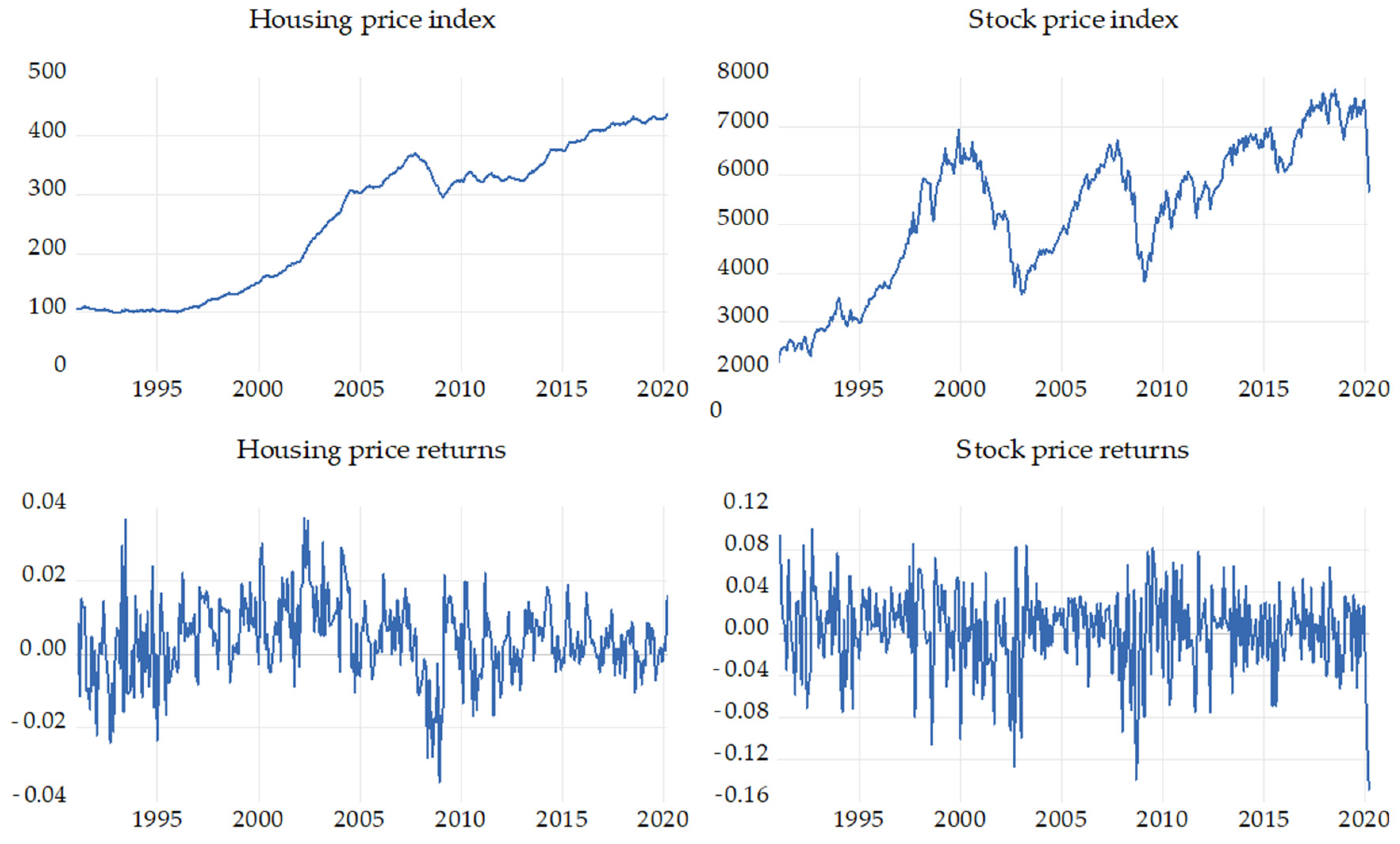
Notes: The labels in the table are explained as follows: housing price index, stock price index, money supply, the real GDP are represented by $\mathit{HP}$, $\mathit{SP}$, $M2$, and $\mathit{GDP}$, respectively.

shows the simple statistics of the variables. Figure 1 shows the historical time series of the housing price index and the stock price index, as well as the returns of the two indices. Table 1 indicates that the housing price index starts from 99 points and reaches 438 points, and the stock price index ranges from 2170 points at the lowest point in the year 1991 to 7748 points at the highest point within the period recorded by data. A comparison of the housing and stock markets indicates that the housing price index changes (maximun-minimun/minimun) are larger within the period recorded by data. The housing price index volatility is not high except for a large rising trend that occurred from the year 1999 to 2007. The housing price index rose sharply three times within the period recorded by data for the years 1993–2000, 2002–2007, and 2009–2015. In addition, two rapid and substantial amendments occurred during 2000–2002 and 2007–2008.

Table 2. Unit root tests.

Variable	$\mathbf{ln}\mathit{HP}$	$\mathbf{ln}\mathit{SP}$	$\mathbf{ln}\mathit{M}2$	$\mathbf{ln}\mathit{GDP}$
Unit Root Test (Variables in Level)
ADF test	−0.8674	−2.7101	−1.4167	−2.3814
	(0.7978)	(0.0733)	(0.5745)	(0.1478)
Lag Length	2	0	0	6
PP test	−0.8129	−2.6996	−1.3844	−1.9468
	(0.8138)	(0.0751)	(0.5904)	(0.3106)
Lag Length	11	6	4	12
Unit Root Test (Variables in Differenced)
ADF test	−7.4986	−17.7484	−17.6943	−3.3267
	(0.0000)	(0.0000)	(0.0000)	(0.0145)
Lag Length	1	0	0	5
PP test	−14.2172	−17.7484	−17.7362	−4.8057
	(0.0000)	(0.0000)	(0.0000)	(0.0001)
Lag Length	9	5	4	10

Notes: The labels in the table are explained as follows: housing price index, stock price index, money supply, the real GDP are represented by $\mathit{HP}$, $\mathit{SP}$, $M2$, and $\mathit{GDP}$, respectively. All variables were transformed using a natural logarithm. ADF and PP tests are adopted for testing the null hypothesis of a unit root in the series. The intercept is included in the testing equation, and the lag length of the unit root models is selected by using the Schwarz information criterion. The entry in parenthesis stands for the p-value. 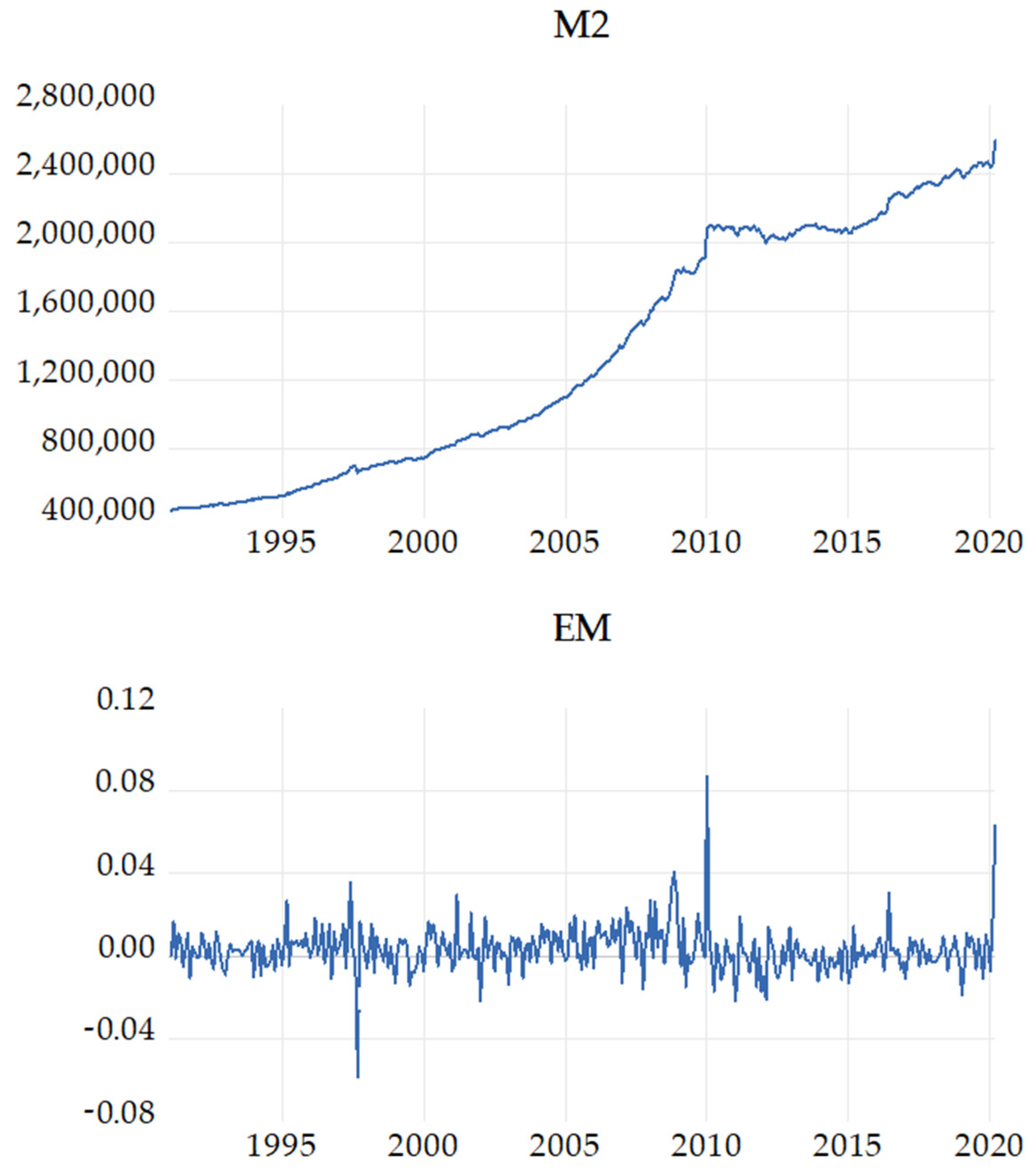The number in bold denotes significance at the 5% level.

also reports the outcome of tests for stationarity. The results of ADF test and PP test all confirm that the variables are I (1), that is the variables are all nonstationary in levels and are all stationary in the first differenced terms. Hence, the housing price return, stock price return, and excess rate of money growth (money supply growth rate minus the economic growth rate) employed in this paper are all stationary data. Figure 2 illustrates money supply and the excess rate of money growth; money supply gradually increased before the year 2008, increased substantially in early 2010, and subsequently remained in a horizontal trend. Moreover, Figure 2 indicates that the most evident excess monetary liquidity appeared in January 2010 (8.69%) and March 2020 (6.34%). The following empirical analysis explains how the changes in excess monetary liquidity influence the linkages among asset markets.

4.2. Empirical Results

To preliminarily understand the relationship between the housing and stock markets,

Table 3. Pairwise Granger Causality Tests.

Null Hypothesis:	F-Statistic	p-Value
Lags: 1
$\Delta \mathit{SP}$ does not Granger Cause $\Delta \mathit{HP}$	0.2293	0.6323
$\Delta \mathit{HP}$ does not Granger Cause $\Delta \mathit{SP}$	0.0456	0.8311
Lags: 2
$\Delta \mathit{SP}$ does not Granger Cause $\Delta \mathit{HP}$	0.5196	0.5952
$\Delta \mathit{HP}$ does not Granger Cause $\Delta \mathit{SP}$	0.3754	0.6873
Lags: 3
$\Delta \mathit{SP}$ does not Granger Cause $\Delta \mathit{HP}$	1.7102	0.1646
$\Delta \mathit{HP}$ does not Granger Cause $\Delta \mathit{SP}$	1.1261	0.3385
Lags: 4
$\Delta \mathit{SP}$ does not Granger Cause $\Delta \mathit{HP}$	1.4253	0.2252
$\Delta \mathit{HP}$ does not Granger Cause $\Delta \mathit{SP}$	1.3373	0.2557

Notes: Housing price returns and stock price returns are represented by $\Delta \mathit{HP}$ and $\Delta \mathit{SP}$, respectively.

lists the causality tests of housing price and stock price returns and presents the causality (Periods 1–4) of various estimated lag periods. The Schwarz information criterion is considered when selecting the lag length of the model. The model with four lags is found to have the optimal goodness of fit. The results shown in Table 3 suggest that all the test results cannot reject the null hypothesis of no causality, indicating that housing price return cannot influence stock price return and that the wealth effect of stock prices on housing prices does not exist.

Subsequently, Equations (6) and (7) were estimated, and the results are presented in

Table 4. Results of Linear Regression.

Variables	$\Delta \mathit{HP}$	$\Delta \mathit{SP}$
$\Delta {\mathit{HP}}_{t-1}$	0.3575	0.0422
	[7.0973]	[0.2135]
$\Delta {\mathit{SP}}_{t-1}$	−0.0067	0.0342
	[−0.4789]	[0.6280]
$\mathit{Constant}$	0.0026	0.0022
	[4.4922]	[0.9612]
Adj. R-squared	0.1221	−0.0045
Log likelihood	1105.3380	627.9712
Akaike information criterion	−6.3171	−3.5815
Schwarz information criterion	−6.2840	−3.5484

Notes: Housing price returns and stock price returns are represented by $\Delta \mathit{HP}$ and $\Delta \mathit{SP}$, respectively. Entry in parenthesis stands for the t-statistics. The number in bold denotes significance at the 5%. The lag length of the model is selected via the Schwarz Information Criterion.

, which indicate that autocorrelation or housing price return from the previous period do not influence stock price returns and that autocorrelation is significantly and positively exhibited in housing price returns. The influence of stock prices from the previous period on housing price returns is still insignificant, probably because the model (Equation (4)) does not consider the dynamic correlation between the housing and stock markets and thus yields a poor goodness-of-fit of the model.

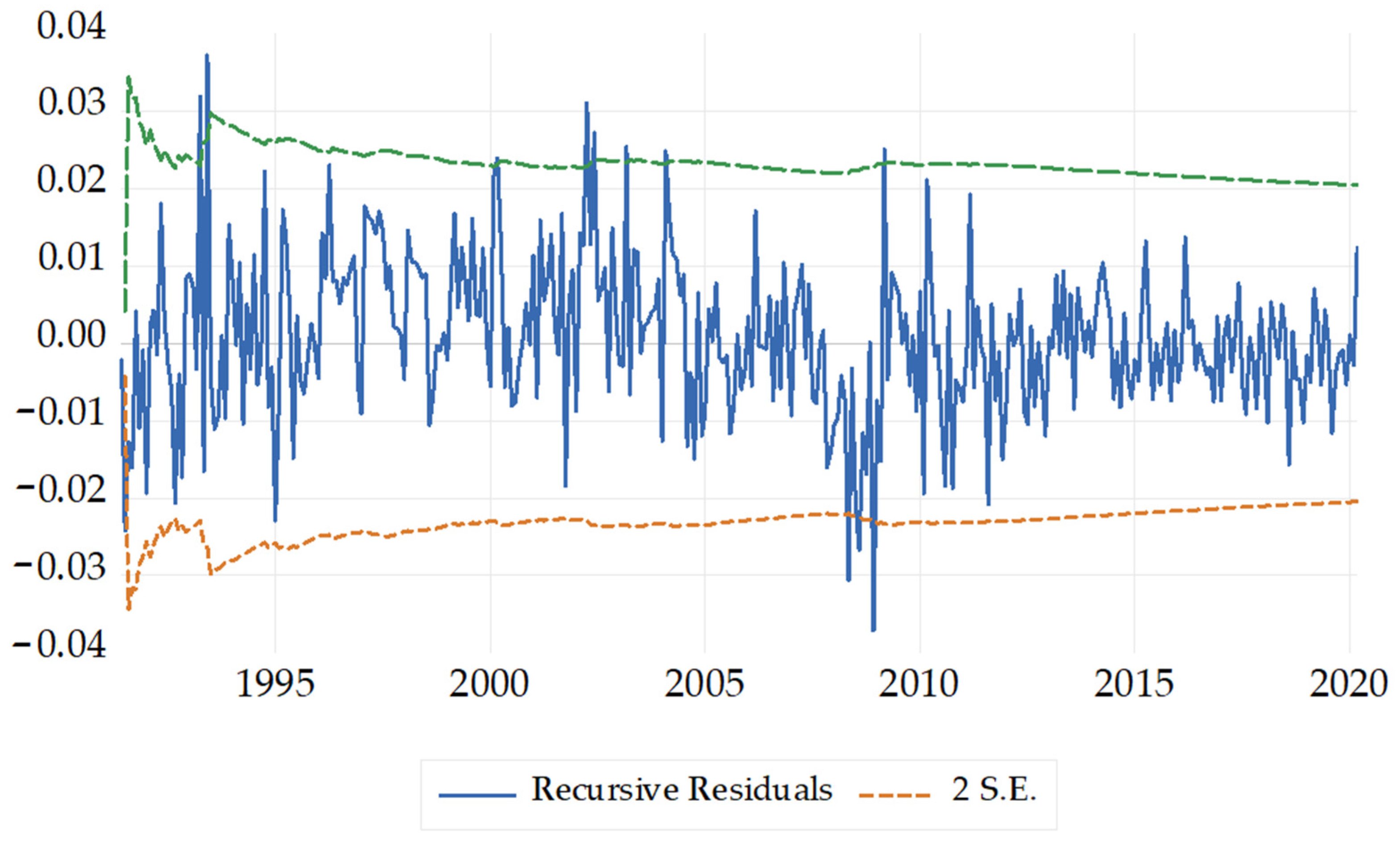
To verify the proposed problems regarding the goodness-of-fit of the model, the recursive residuals are illustrated in Figure 3. Galpin and Hawkiws [55] proposed a comparison between recursive residuals and residuals of normal distribution, through which potential problems in changes of regimes, outliers, and omitted predictors in the model can be examined and whether these problems prevented the goodness-of-fit from being correctly estimated can be analyzed. Figure 3 shows the recursive residuals estimated in the model. Plus and minus two standard errors are also shown in Figure 3, based on the assumption of normal distribution, the estimated residuals from the OLS model outside the standard error bands suggest instability in the parameters of the equation. Figure 3 shows that many points in time exceed the theoretically estimated values, exceeding two times the standard deviation; thus, the goodness-of-fit of this linear model is poor.

Several factors can cause poor goodness-of-fit in the aforementioned model. The CUSUM test (Brown et al., [54]) is continuously employed to examine whether a low goodness-of-fit is caused by structural changes of the estimated coefficients. The CUSUM test is based on recursive residuals (standardized forecast errors), which are estimated by using the OLS model for coefficients from the $t-1$ observations. When the test statistic (the cumulated sum of the recursive residuals exceeds the corresponding critical value, the null hypothesis of parameter constancy is rejected. The CUSUM of the recursive residuals for the model and the corresponding critical value are illustrated in Figure 4, which indicate that the accumulated residual values from 1999M12 to 2008M11 exceed the expected range. Therefore, the coefficients of the model within this period may be inconsistent with the estimated coefficients in other periods, suggesting that the relationship between housing and stock markets may be changeable.

Table 5. Results from the Model Inclusion of the Excess Rate of Money Growth.

Variables	$\Delta \mathit{HP}$
$\Delta {\mathit{HP}}_{t-1}$	0.3274
	[5.7962]
${\mathit{EM}}_{t-1}\times \Delta {\mathit{HP}}_{t-1}$	4.6524
	[1.0764]
$\Delta {\mathit{SP}}_{t-1}$	−0.0165
	[−1.1473]
${\mathit{EM}}_{t-1}\times \Delta {\mathit{SP}}_{t-1}$	2.7180
	[2.6393]
$\mathit{Constant}$	0.0028
	[4.8693]
Adj. R-squared	0.1399
Log likelihood	1109.9382
Akaike information criterion	−6.3320
Schwarz information criterion	−6.2768

Notes: Housing price returns and stock price returns are represented by $\Delta \mathit{HP}$ and $\Delta \mathit{SP}$, respectively. $\mathit{EM}$ represents the excess rate of money growth. Entry in parenthesis stands for the t-statistics. The number in bold denotes significance at the 5% level. The lag length of the model is selected via the Schwarz Information Criterion. The estimated model is: ${\Delta \mathit{HP}}_t=C_0+C_1{\Delta \mathit{HP}}_{t-1}+C_2{\mathit{EM}}_{t-1}\times {\Delta \mathit{HP}}_{t-1}+C_3{\Delta \mathit{SP}}_{t-1}+C_4{\mathit{EM}}_{t-1}\times {\Delta \mathit{SP}}_{t-1}+{\epsilon }_t$.

estimates Equation (8) to determine whether the excess rate of money growth of the linear model should be incorporated to estimate a high goodness-of-fit. The results in Table 5 suggest that the autocorrelation of housing price return is not influenced by the excess rate of money growth because $C_2$ is insignificant. Table 5 also indicates that $C_4$ is extremely significant and is a positive value (2.718), showing that the excess rate of money growth significantly influences the relationship between housing price return and stock price return from the previous period. A large excess rate of money growth increases the wealth effect of the stock market on the housing market. When the excess rate of money growth is 0, the stock market does not influence the housing market. This may be explained by the mutual offset between the crowding out of capital and the wealth effect in different industries, which is implied by Equation (3). When the excess rate of money growth is negative, the influence of stock price return from the previous period on housing price return is negative; therefore, the wealth effect no longer exists, and only the capital switching effect remains.

From the results in Table 5, whether the effect of excess monetary liquidity exists can be observed; in other words, whether the excess rate of money growth is larger than 0 determines whether the wealth effect or capital switching effect can exist. To verify the effect of excess monetary liquidity, which is a crucial factor, the following equation was estimated:

$${\Delta \mathit{HP}}_t=C_0+C_1{\Delta \mathit{HP}}_{t-1}+C_2{\Delta \mathit{SP}}_{t-1}+C_3{\mathit{Dummy}}_{t-1}{\mathit{EM}}_{t-1}\times {\Delta \mathit{SP}}_{t-1}+{\epsilon }_t.$$

(15)

In the aforementioned equation, a dummy variable (${\mathit{Dummy}}_t$) > 0 in the excess rate of money growth is incorporated. When ${\mathit{EM}}_t$ > 0, ${\mathit{Dummy}}_t$ = 1 or 0 otherwise. In Equation (15), the influence of the excess rate of money growth on the relationship between the housing and stock markets is measured only when excess monetary liquidity exists (i.e., when ${\mathit{EM}}_t$ > 0).

Table 6. Results from the Model Inclusion of the Effect of Excess Monetary Liquidity.

Variables	$\Delta \mathit{HP}$
$\Delta {\mathit{HP}}_{t-1}$	0.3539
	[7.1056]
$\Delta {\mathit{SP}}_{t-1}$	−0.0357
	[−2.1305]
${Dummy}_{t-1}\times {EM}_{t-1}\times \Delta {SP}_{t-1}$	4.3645
	[3.0180]
$Constant$	0.0029
	[4.9131]
Adj. R-squared	0.1422
Log likelihood	1109.8851
Akaike information criterion	−6.3375
Schwarz information criterion	−6.2933

Notes: Housing price returns and stock price returns are represented by $\Delta HP$ and $\Delta SP$, respectively. $EM$ represents the excess monetary liquidity. $Dummy$ is a dummy variable, which equals to 1 denotes the existence of the excess monetary liquidity. Entry in parenthesis stands for the t-statistics. The number in bold denotes significance at the 5% level. The lag length of the model is selected via the Schwarz Information Criterion. The estimated model is: $\Delta {HP}_t=C_0+C_1\Delta {HP}_{t-1}+C_2\Delta {SP}_{t-1}+C_3{Dummy}_{t-1}{EM}_{t-1}\times \Delta {SP}_{t-1}+{\epsilon }_t$.

presents the results.

The results shown in Table 6 correspond with our inference, and the goodness-of-fit of the model (Adj $R^2$) is drastically superior to that shown in Table 4 and Table 5. When excess monetary liquidity does not exist (i.e., when ${\mathit{EM}}_t$ ≤ 0), the stock price return from the previous period significantly and negatively influences housing price return (the coefficient = −0.0357), indicating that the capital switching effect exists between the housing and stock markets in these conditions. When excess monetary liquidity occurs (i.e., when ${\mathit{EM}}_t$ > 0), the stock price return from the previous period significantly and positively influences housing price return (the coefficient = 4.3645), and the extent of this positive influence is affected by the excess rate of money growth. Thus, the wealth effect exists between the housing and stock markets in these conditions, and a large excess liquidity indicates a strong wealth effect.

Table 7. Results of the TVC Model.

Variables	Coefficient	Standard Error	t-Statistic	p-Value
$a_0$	0.4270	0.0129	33.1400	0.0000
$a_1$	0.7349	1.1056	0.6647	0.5067
$a_2$	0.7360	1.1090	0.6639	0.5072
$b_0$	−0.0125	0.0027	−4.7259	0.0000
$b_1$	0.4758	0.2277	2.0895	0.0374
$b_2$	0.5286	0.2284	2.3143	0.0212

Notes: Housing price returns and stock price returns are represented by $\Delta \mathit{HP}$ and $\Delta \mathit{SP}$, respectively. $\mathit{EM}$ represents the excess monetary liquidity. The number in bold denotes significance at the 5% level. The lag length of the model is selected via the Schwarz Information Criterion. The estimated model is: ${\Delta \mathit{HP}}_t={\alpha }_t{\Delta \mathit{HP}}_{t-1}+{\beta }_t{\Delta \mathit{SP}}_{t-1}+{\epsilon }_t$, where ${\alpha }_t=a_0+a_1{\mathit{EM}}_{t-1}+a_2{\mathit{EM}}_{t-2}+u_{1t}$; ${\beta }_t=b_0+b_1{\mathit{EM}}_{t-1}+b_2{\mathit{EM}}_{t-2}+u_{2t}$.

presents the estimated results of the TVC model and suggests that the autocorrelation in housing price return exhibits no time-varying characteristics because only the constant term in the equation of the autocorrelation coefficient (${\alpha }_t$) is significant, and it is a significantly positive value (0.427). Therefore, housing price return is influenced by the return from the previous period, an influence 0.427 fold, and this influence exhibits no changes according to the currency level within the period shown in the data. In addition, the influence of stock price return from the previous period on housing price return changes according to time. Regarding the coefficient (${\beta }_t$) equation that indicates the effect of the stock market on the housing market, all the coefficients are significantly differ from 0. The constant term is close to zero (−0.01), hence the effect is mainly influenced by the excess rate of money growth from the previous period and the period before the previous one, in which the coefficients are all positive and are approximately 0.5. If the currency in the previous two periods exhibited no excess liquidity, then the stock market and the housing market may only have little connection (i.e., ${\mathit{EM}}_t$ = 0, ${\mathit{\beta }}_t$ = −0.01). Moreover, if ${\mathit{EM}}_t$ < 0, the stock market may negatively influence the housing market. Hence, the capital switching effect existed. The results in Table 7 are consistent with those in Table 6. However, the estimated results of the TVC model clearly explain how the influence of the stock market on the housing market is determined. The results of Table 7 also consistent with the findings of Lee et al. [17]. Lee et al. [17] provided the evidence showing the existence of capital switching activities between housing and stocks, and the relationships between Australian house prices and stock prices can vary depending on the market conditions.

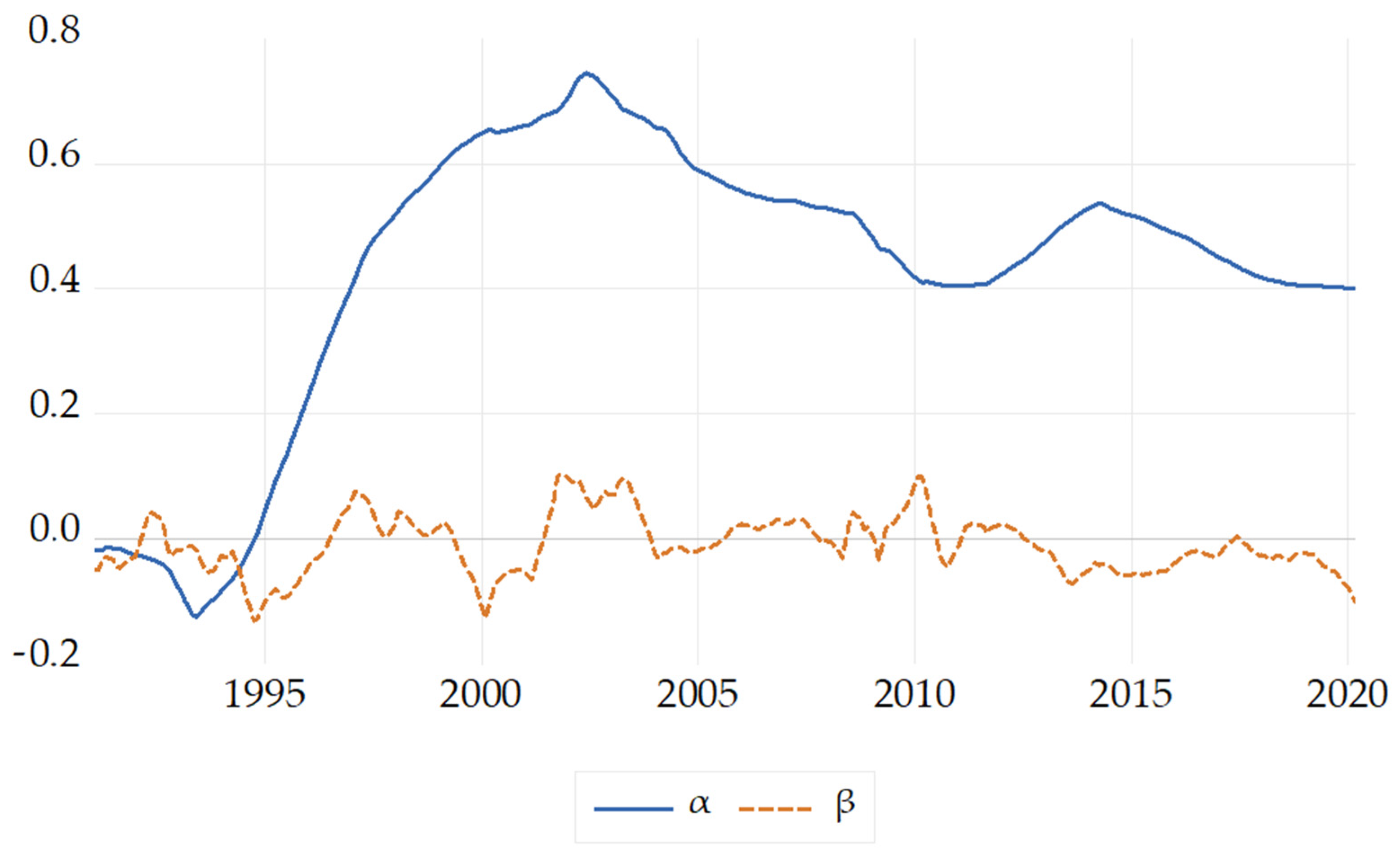
Figure 5 illustrates the model’s estimated autocorrelation coefficient (${\alpha }_t$) and the coefficient (${\beta }_t$) that indicates the influential effect of stock markets on housing markets. The changes in ${\alpha }_t$ are minor, but a crucial turning point occurred around 2002. From 1993 to 2002, the autocorrelation coefficient of housing price gradually increased. The autocorrelation coefficient was originally negative in 1993, became positive in 1995, and almost remained at a level higher than 0.5 after 1998. A positive autocorrelation indicates the momentum of housing price changes; in other words, when housing price rises, a positive autocorrelation enables housing price to continuously increase, exhibiting a drastically rising trend in housing price. The estimated results are consistent with the price trends of UK housing and stock market in Figure 1. Figure 1 indicates that an evident rising trend in housing price in the UK started in 1999; specifically, before 1995, housing price exhibited a negative autocorrelation, and housing price return fluctuated, thereby preventing the formation of a rising trend. By comparison, Figure 2 shows that the excess monetary liquidity before 1995 was minor; thus, the relationship between housing and stock markets should involve a crowding out of capital according to the estimated results in Table 7. The stock market shown in Figure 1 suggests that an upward wave pattern already existed before 1995.

Regarding the coefficient (${\beta }_t$) that indicates the influential effect of the stock market on the housing market, Figure 5 clearly illustrates the period in which the wealth effect and capital switching effect were present. For example, the capital switching effect was present in the housing and stock markets before 1996, and the wealth effect subsequently appeared from 1996 to 1999. From 1999 to 2001, the capital switching effect was present in the two markets; from 2001 to 2003, the wealth effect emerged in the two markets; after 2003, the wealth and capital switching effects in the two markets became insignificant. However, from 2008 to 2010, the wealth effect was evidently present during two periods. Figure 2 shows that the two periods of substantial monetary easing occurred from 2008 to mid-2010; specifically, data indicate that the largest excess monetary liquidity in a single month occurred from late 2009 to early 2010, in which a rate of 8.69% was obtained after subtracting the economic growth rate from the money supply rate. This substantial stimulus also caused both the housing and stock markets to rebound sharply and fueled housing and stock price. The patterns of the coefficient (${\beta }_t$) show the similar findings with that of Lee et al. [17]. Lee et al. [17] well documented the impact of the global financial crisis on the relationships between house prices and stock prices, especially, the capital switching effect was existed during the periods of the global financial crisis happened. The empirical results of this paper not only supported the findings of the previous studies, but also provided substantial evidence showing that excess monetary liquidity is a crucial factor in determining the effect of the stock market on the housing market.

Relevant studies (Quan and Titman, [56]; Green, [34]) found that the relationship between the stock market and housing market may differ because of the use of housing market data from different regions. To verify the inference of this study more strictly, the results of using the TVC model to estimate relations between the housing markets and stock markets in 13 regions in the United Kingdom are listed in

Table 8. Regional Results of the TVC Model.

Variables	North	Yorkshire and the Humber	North West	East Midlands	West Midlands
$a_0$	−0.0101	0.1978	0.3142	0.5298	0.5810
	[−0.3488]	[7.3945]	[11.7636]	[16.9694]	[28.1813]
$a_1$	1.8117	2.2367	1.3826	0.8181	0.1109
	[1.5015]	[1.9994]	[1.2377]	[0.6266]	[0.1286]
$a_2$	2.0958	2.2844	1.5676	0.4224	−0.2208
	[1.6730]	[1.9667]	[1.3516]	[0.3116]	[−0.2467]
$b_0$	0.0325	0.0277	0.0350	0.0314	0.0087
	[3.6473]	[2.2133]	[6.9245]	[4.0868]	[1.8171]
$b_1$	1.4258	0.6614	0.7333	0.4928	0.3824
	[3.8228]	[1.2639]	[3.4688]	[1.5341]	[1.9100]
$b_2$	1.8106	0.5960	0.8992	0.1405	0.3482
	[4.6758]	[1.0971]	[4.0968]	[0.4213]	[1.6749]
	East Anglia	Outer South East	Outer Metropolitan	London	South West
$a_0$	0.4759	0.6629	0.7071	0.5157	0.5836
	[19.4926]	[34.7303]	[99.6617]	[29.9516]	[37.9633]
$a_1$	0.9303	0.2285	0.1073	−0.0011	0.2801
	[0.9110]	[0.2863]	[0.3615]	[−0.0015]	[0.4357]
$a_2$	1.0549	0.1483	0.0360	−0.0335	0.3372
	[0.9950]	[0.1789]	[0.1167]	[−0.0448]	[0.5052]
$b_0$	0.0861	0.0135	−0.0077	0.0322	0.0643
	[9.4411]	[1.7317]	[−1.0217]	[2.7597]	[9.8752]
$b_1$	0.2900	0.8984	0.7776	1.1738	−0.1841
	[0.7603]	[2.7460]	[2.4582]	[2.4078]	[−0.6760]
$b_2$	0.0242	0.5972	0.7202	0.7643	0.1188
	[0.0610]	[1.7583]	[2.1926]	[1.5099]	[0.4202]
	Wales	Scotland			North Ireland
$a_0$	0.1016	0.2388			0.1630
	[2.7985]	[8.3847]			[4.8746]
$a_1$	0.5166	1.7459			3.6293
	[0.3401]	[1.4657]			[2.5950]
$a_2$	−0.0654	1.6942			3.8148
	[−0.0415]	[1.3699]			[2.6271]
$b_0$	0.0310	0.0381			0.1006
	[2.6125]	[3.8628]			[6.6410]
$b_1$	1.0985	0.4389			0.9353
	[2.2167]	[1.0646]			[1.4764]
$b_2$	0.6344	0.8765			1.0111
	[1.2329]	[2.0476]			[1.5371]

Notes: Housing price returns and stock price returns are represented by $\Delta \mathit{HP}$ and $\Delta \mathit{SP}$, respectively. $\mathit{EM}$ represents the excess monetary liquidity. The number in bold denotes significance at the 5% level. The lag length of the model is selected via the Schwarz Information Criterion. The estimated model is: ${\Delta \mathit{HP}}_t={\alpha }_t{\Delta \mathit{HP}}_{t-1}+{\beta }_t{\Delta \mathit{SP}}_{t-1}+{\epsilon }_t$, where ${\alpha }_t=a_0+a_1{\mathit{EM}}_{t-1}+a_2{\mathit{EM}}_{t-2}+u_{1t}$; ${\beta }_t=b_0+b_1{\mathit{EM}}_{t-1}+b_2{\mathit{EM}}_{t-2}+u_{2t}$.

. The table reveals that when the regional housing markets are examined, excessive liquidity still has an extremely large influence. Table 8 also indicates that the stock market has an increasingly positive influence on the housing market when the money has excessive liquidity in a total of seven regions. For two of the other regional housing markets, when the money has excessive liquidity, the housing prices tend to increase. Finally, in only four regional housing markets (the East Midlands, West Midlands, South West, and East Anglia), the housing and stock markets are not influenced by the excessive liquidity of money. In the West Midlands, the housing and stock markets are independent of each other. This may be because housing markets with certain characteristics (such as high prices) are not related to the stock market (Bangura and Lee, [19]). This study finds that the house prices in some regions are not related to the stock prices. A possible reason is that this study uses samples that include the home price indices of all transactions (for both living and investment needs), and it does not just discuss the transactions for the investment need. Dieci and Westerhoff [57], Lee et al. [17], Pawson and Martin [58], Bangura and Lee [59] all study investor behaviors in housing markets. These behaviors are found to influence the risks and returns of the house prices. Therefore, the house prices effects that only consider the investors may be more related to the stock prices.

5. Conclusions

This paper offers a new perspective and evidence on the topic of housing and stock markets. Data on stock price return, housing price return, and the excess rate of money growth (economic growth rate subtracted from the increased rate of money supply) from January 1991 to March 2020 in the UK are employed to verify whether excess monetary liquidity (when the excess rate of money growth > 0) is key in determining the relationship between housing and stock markets.

First, through a literature review, we determined that the influence of the stock market on the housing market can be easily observed and that two effects may coexist: the wealth and capital switching effects. The quantity theory of money is employed to explain that the capital in the housing and stock markets (industries) may generate a mutual crowding out effect when money supply does not increase, similar to the model of capital investment proposed by Harvey [42] for the three circuits. A substantial increase of money supply in the short-term (before output increases) results in excess monetary liquidity, enabling different markets (industries) to attract capital for investment without competition, resulting in mutual fueling (the occurrence of the wealth effect). Capital transfer can prevent autocorrelation from occurring during excessive market investment and thereby aggravate market imbalance.

Empirically, we determined that using linear regression to estimate the dynamic relationship between housing and stock markets is erroneous and can easily underestimate the influence of stock markets on housing markets. Incorporating a model with a variable for excess monetary liquidity can offer favorable explanatory power, explain whether excess monetary liquidity exists, and determine whether the wealth or capital switching effects substantially influence excess monetary liquidity.

The influence of stock price return from the previous period on housing price return is affected by whether excess monetary liquidity previously existed. Specifically, we employed the TVC model for estimation and determined that, regarding the coefficient (${\beta }_t$) equation that indicated the influential effect of stock markets on housing markets, the estimated constant term is significantly differ from 0 and slightly negative, suggesting that if money supply is reduced and no excess monetary liquidity exists (the excess rate of money growth is a negative value), then the two markets are negatively related. Namely, the capital switching effects dominate between housing and stock markets. If money supply increases substantially (e.g., the quantitative easing in late 2009 and early 2010), then capital is invested in the housing and stock markets, and the wealth effect is thus generated. During this period, the stock market rally benefited the housing market recovery.

The proposed theoretical and empirical results in this paper explain the role that the wealth and capital switching effects play in excess monetary liquidity as well as the importance of monetary policy in asset market linkages. This paper also shows that a reduced crowding out effect of capital causes the mechanism for amending an imbalanced single market to disappear, a major reason for the expansion of financial crises. When excess monetary liquidity is not present, capital transfer in markets can inhibit the bubble of a single market and not only prevent a large-scale financial crisis in this market from easily forming but also avoid extensive chaos across financial markets.

This paper verifies that excess monetary liquidity influences market-related matters (risk transfer). We recommend that future studies analyze the influence that the absence of capital switching effect has on the probability of forming a financial crisis and also consider the scale of the potential financial crisis. In addition, subsequent studies are recommended to additionally consider consumption in the model to quantify the capital switching effect more precisely. The results also indicate the importance of central banks in each country while strictly controlling for monetary policy because the major goal of this policy is to first ensure financial stability and then promote economic growth.

References

1. McDonald, J.F.; Stokes, H.H. Monetary policy, mortgage rates and the housing bubble. Econ. Financ. Res. 2013, 1, 82–91. [Google Scholar] [CrossRef] [Green Version]
2. Roffia, B.; Zaghini, A. Excess money growth and inflation dynamics. Int. Financ. 2007, 10, 241–280. [Google Scholar] [CrossRef]
3. Brana, S.; Djigbenou, M.-L.; Prat, S. Global excess liquidity and asset prices in emerging countries: A PVAR approach. Emerg. Mark. Rev. 2012, 13, 256–267. [Google Scholar] [CrossRef] [Green Version]
4. Brounen, D.; Eichholtz, P.M.A. Property, common stock, and property shares. J. Portf. Manag. 2003, 29, 129–137. [Google Scholar] [CrossRef]
5. Kallberg, J.G.; Liu, C.H.; Pasquariello, P. Regime shifts in Asian equity and real estate markets. Real Estate Econ. 2002, 30, 263–291. [Google Scholar] [CrossRef]
6. Hui, E.C.M.; Zuo, W.; Hu, L. Examining the relationship between real estate and stock markets in Hong Kong and the United Kingdom through datamining. Int. J. Strateg. Prop. Manag. 2011, 15, 26–34. [Google Scholar] [CrossRef]
7. Tsai, I.-C.; Lee, C.-F.; Chiang, M.-C. The asymmetric wealth effect in the US housing and stock markets: Evidence from the threshold cointegration model. J. Real Estate Financ. Econ. 2012, 45, 1005–1020. [Google Scholar] [CrossRef]
8. Wilson, P.; Okunev, J. Long-term dependencies and long run non-periodic co-cycles: Real estate and stock markets. J. Real Estate Res. 1999, 18, 257–278. [Google Scholar]
9. Markowitz, H. Portfolio selection. J. Financ. 1952, 7, 77–91. [Google Scholar]
10. Liu, C.H.; Hartzell, D.J.; Greig, W.; Grissom, T.V. The integration of the real estate market and the stock market: Some preliminary evidence. J. Real Estate Financ. Econ. 1990, 3, 261–282. [Google Scholar] [CrossRef]
11. Ong, S.E. Singapore real estate and property stocks—A cointegraton test. J. Prop. Res. 1995, 12, 29–39. [Google Scholar]
12. Wilson, P.; Zurbruegg, R. Contagion or interdependence? Evidence from co-movements in Asia-Pacific securitized real estate markets during the 1997 crisis. J. Prop. Investig. Financ. 2004, 22, 401–413. [Google Scholar] [CrossRef]
13. Bond, S.A.; Dungey, M.; Fry, R. A web of shocks: Crisis across Asia-Pacific region real estate markets. J. Real Estate Financ. Econ. 2006, 32, 253–274. [Google Scholar] [CrossRef]
14. Liow, K.H. Financial crisis and Asian real estate securities market interdependence: Some additional evidence. J. Prop. Res. 2008, 25, 127–155. [Google Scholar] [CrossRef]
15. De Bandt, O.; Barhoumi, K.; Bruneau, C. The international transmission of house price shocks. In Housing Markets in Europe; Springer: Berlin/Heidelberg, Germany, 2010; pp. 129–158. [Google Scholar]
16. Chiang, M.-C.; Tsai, I.-C. Ripple and contagion effects in U.S. regional housing markets. Ann. Reg. Sci. 2016, 56, 55–82. [Google Scholar] [CrossRef]
17. Lee, M.-T.; Lee, C.L.; Lee, M.-L.; Liao, C.-Y. Price linkages between Australian housing and stock markets: Wealth effect, credit effect or capital switching? Int. J. Hous. Mark. Anal. 2017, 10, 305–323. [Google Scholar] [CrossRef]
18. Lee, C.L. An examination of the risk-return relation in the Australian housing market. Int. J. Hous. Mark. Anal. 2017, 10, 431–449. [Google Scholar] [CrossRef]
19. Bangura, M.; Lee, C.L. House price diffusion of housing submarkets in Greater Sydney. Hous. Stud. 2020, 35, 1110–1141. [Google Scholar] [CrossRef]
20. Son, J.C.; Park, H. The effects of regional house prices on consumption in Korea: Heterogeneous behaviors according to homeownership status and lifecycle stage. Sustainability 2020, 12, 3517. [Google Scholar] [CrossRef]
21. Guo, F.; Huang, Y.S. Does “hot money” drive China’s real estate and stock markets? Int. Rev. Econ. Financ. 2010, 19, 452–466. [Google Scholar] [CrossRef]
22. Xu, X.E.; Chen, T. The effect of monetary policy on real estate price growth in China. Pac.-Basin Financ. J. 2012, 20, 62–77. [Google Scholar] [CrossRef]
23. Zhu, B.; Betzinger, M.; Sebastian, S. Housing market stability, mortgage market structure, and monetary policy: Evidence from the euro area. J. Hous. Econ. 2017, 37, 1–21. [Google Scholar] [CrossRef] [Green Version]
24. Su, C.-W.; Wang, X.-Q.; Tao, R.; Chang, H.-L. Does money supply drive housing prices in China? Int. Rev. Econ. Financ. 2019, 60, 85–94. [Google Scholar] [CrossRef]
25. Tsai, I.C.; Chiang, S.-H. Risk transfer among housing markets in major cities in China. Sustainability 2018, 10, 2386. [Google Scholar] [CrossRef] [Green Version]
26. Hu, L.; Han, J.; Zhang, Q. The impact of monetary and fiscal policy shocks on stock markets: Evidence from China. Emerg. Mark. Financ. Trade 2018, 54, 1856–1871. [Google Scholar] [CrossRef]
27. Lütkepohl, H.; Netšunajev, A. The relation between monetary policy and the stock market in Europe. Econometrics 2018, 6, 36. [Google Scholar] [CrossRef] [Green Version]
28. Ando, A.; Modigliani, F. The life cycle hypothesis of saving: Aggregate implications and tests. Am. Econ. Rev. 1963, 53, 55–84. [Google Scholar]
29. Yoshikawa, H.; Ohtaka, F. An analysis of female labor supply, housing demand and the saving rate in Japan. Eur. Econ. Rev. 1989, 33, 997–1023. [Google Scholar] [CrossRef]
30. Case, K.E. The real estate cycle and the economy: Consequences of the Massachusetts boom of 1984–1987. Urban Stud. 1992, 29, 171–183. [Google Scholar] [CrossRef]
31. Poterba, J.M. Stock market wealth and consumption. J. Econ. Perspect. 2000, 14, 91–118. [Google Scholar] [CrossRef]
32. Lusardi, A.; Mitchell, O.S. Baby boomer retirement security: The roles of planning, financial literacy, and housing wealth. J. Monet. Econ. 2007, 54, 205–224. [Google Scholar] [CrossRef] [Green Version]
33. Dvornak, N.; Kohler, M. Housing wealth, stock market wealth and consumption: A panel analysis for Australia. Econ. Rec. 2007, 83, 117–130. [Google Scholar] [CrossRef]
34. Green, R.K. Stock prices and house prices in California: New evidence of a wealth effect? Reg. Sci. Urban Econ. 2002, 32, 775–783. [Google Scholar] [CrossRef]
35. Okunev, J.; Wilson, P.; Zurbruegg, R. Relationships between Australian real estate and stock market prices: A case of market inefficiency. J. Forecast. 2002, 21, 181–192. [Google Scholar] [CrossRef]
36. Su, C.W. Non-linear causality between the stock and real estate markets of Western European countries: Evidence from rank tests. Econ. Model. 2011, 28, 845–851. [Google Scholar] [CrossRef]
37. Kapopoulos, P.; Siokis, F. Stock and real estate prices in Greece: Wealth versus ‘credit-price’ effect. Appl. Econ. Lett. 2005, 12, 125–128. [Google Scholar] [CrossRef]
38. Huang, Y.-K.; Lee, C.-H. Wealth versus credit-price effect in Taiwan. Appl. Sci. Manag. Res. 2014, 1, 102–111. [Google Scholar]
39. McMillan, D. Long-run stock price-house price relation: Evidence from an ESTR model. Econ. Bull. 2012, 32, 1737–1746. [Google Scholar] [CrossRef] [Green Version]
40. Yousaf, I.; Ali, S. Integration between real estate and stock markets: New evidence from Pakistan. Int. J. Hous. Mark. Anal. 2020, in press. [Google Scholar] [CrossRef]
41. Lizieri, C.; Satchell, S. Interactions between property and equity markets: An investigation of linkages in the United Kingdom 1972–1992. J. Real Estate Financ. Econ. 1997, 15, 11–26. [Google Scholar] [CrossRef]
42. Harvey, D. The urban process under capitalism: A framework for analysis. Int. J. Urban Reg. Res. 1978, 2, 101–131. [Google Scholar] [CrossRef]
43. Beauregard, R.A. Capital switching and the built environment: United States, 1970–89. Environ. Plan. A 1994, 26, 715–732. [Google Scholar] [CrossRef]
44. Sousa, R.M. Housing wealth, financial wealth, money demand and policy rule: Evidence from the euro area. N. Am. J. Econ. Financ. 2010, 21, 88–105. [Google Scholar] [CrossRef]
45. Baks, K.; Kramer, C.F. Global Liquidity and Asset Prices: Measurement, Implications, and Spillovers; IMF Working Papers 99/168; International Monetary Fund: New York, NY, USA, 1999. [Google Scholar]
46. Belke, A.S.; Orth, W. Global Excess Liquidity and House Prices—A VAR Analysis for OECD Countries; Ruhr Economic Papers No. 37; Heinisch-Westfälisches Institut für Wirtschaftsforschung (RWI): Essen, Germany, 2007. [Google Scholar]
47. Guo, S.; Li, C. Excess liquidity, housing price booms and policy challenges in China. China World Econ. 2011, 19, 76–91. [Google Scholar] [CrossRef]
48. Fenig, G.; Mileva, M.; Petersen, L. Deflating asset price bubbles with leverage constraints and monetary policy. J. Econ. Behav. Organ. 2018, 155, 1–27. [Google Scholar] [CrossRef] [Green Version]
49. Bao, T.; Zong, J. The impact of interest rate policy on individual expectations and asset bubbles in experimental markets. J. Econ. Dyn. Control 2019, 107, 103735. [Google Scholar] [CrossRef]
50. Bolt, W.; Demertzis, M.; Diks, C.; Hommes, C.; van der Leij, M. Identifying booms and busts in house prices under heterogeneous expectations. J. Econ. Dyn. Control 2019, 103, 234–259. [Google Scholar] [CrossRef] [Green Version]
51. Galí, J.; Giusti, G.; Noussair, C.N. Monetary Policy and Asset Price Bubbles: A Laboratory Experiment; Barcelona GSE Working Paper No. 1726; Barcelona Graduate School of Economics: Barcelona, Spain, 2020. [Google Scholar]
52. Said, S.E.; Dickey, D.A. Testing for unit roots in autoregressive-moving average models of unknown order. Biometrika 1984, 71, 599–607. [Google Scholar] [CrossRef]
53. Phillips, P.C.B.; Perron, P. Testing for a unit root in time series regression. Biometrika 1988, 75, 335–346. [Google Scholar] [CrossRef]
54. Brown, R.L.; Durbin, J.; Evans, J.M. Techniques for testing the constancy of regression relationships over time. J. R. Stat. Soc. 1975, 37, 149–192. [Google Scholar] [CrossRef]
55. Galpin, J.S.; Hawkins, D.M. The use of recursive residuals in checking model fit in linear regression. Am. Stat. 1984, 38, 94–105. [Google Scholar]
56. Quan, D.C.; Titman, S. Commercial real estate prices and stock market returns: An international analysis. Financ. Anal. J. 1997, 53, 21–34. [Google Scholar] [CrossRef] [Green Version]
57. Dieci, R.; Westerhoff, F. A simple model of a speculative housing market. J. Evol. Econ. 2012, 22, 303–329. [Google Scholar] [CrossRef] [Green Version]
58. Pawson, H.; Martin, C. Rental property investment in disadvantaged areas: The means and motivations of Western Sydney’s new landlords. Hous. Stud. 2020, in press. [Google Scholar] [CrossRef]
59. Bangura, M.; Lee, C.L. Housing price bubbles in Greater Sydney: Evidence from a submarket analysis. Hous. Stud. 2020, in press. [Google Scholar] [CrossRef]
Figure 1. Time Series of the Housing and Stock Markets.
Sustainability 12 08989 g001
Figure 2. Money Supply and the Excess Rate of Money Growth.
Sustainability 12 08989 g002
Figure 3. Results of Model Stability Test.
Sustainability 12 08989 g003
Figure 4. Results of the cumulative sums (CUSUM) Test.
Sustainability 12 08989 g004
Figure 5. Time-Varying Effects.
Sustainability 12 08989 g005