Living Cost Gap in the European Union Member States


Abstract
1. Introduction
- Develop flexible LCG identification framework, which could help decisions-makers in preparation of LCG mitigation measures;
- Identify LCG change trends across MS;
- Provide solution to identify which criterion (and under which circumstances) become more important for identification of LCG;
- Estimate and evaluate relationship between compound annual growth rates (CAGR) of LCG and CAGR of each criterion, across MS.
2. Materials and Methods
2.1. Study Area and Source Data Preparation
- Hypothetical distance from household: adjacent, neighbouring, and distant;
- Economic decision scale relationship with household: micro, mezzo, macro;
- Location effect on household: local, national, international;
- Impact of decision makers on household: individual, external.
- Adjacent–micro–local–individual (e.g., household net earnings, savings);
- Neighbouring–mezzo–national–external (e.g., GDP, labour market, housing availability);
- Distant–macro–international–external (e.g., migration, remittance flows, trade flows);
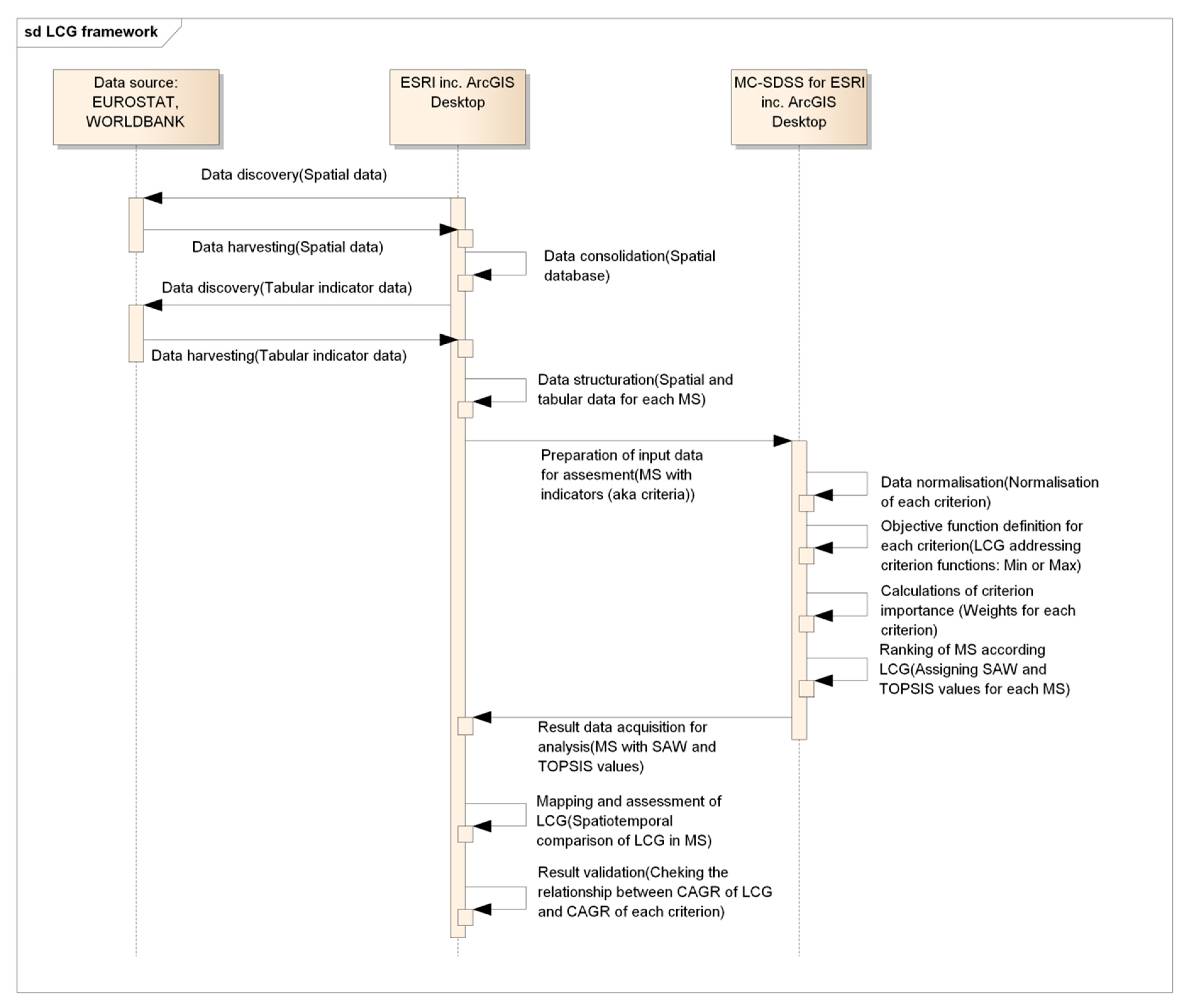
2.2. The LCG Assessment Framework
2.3. Definition of LCG Using Objective Functions
- Households with lowest (minimisation) net income and lowest savings;
- Households with highest (maximisation) expenditures on basic needs (housing, food, and transport) to maintain a minimum level of survival only;
- Households with lowest (minimisation) expenditures on optional needs (education, health, clothing, other miscellaneous goods, etc.);
- Households that are exposed to few employment opportunities and low GDP. MS where unemployment, low work intensity, and income poverty rates are the highest (maximisation) and GDP is lowest (minimisation);
- Households that are exposed to housing gap issues. MS where the housing cost overburden rate and the prevalence of rented houses are the highest (maximisation) and home ownership is the lowest (minimisation);
- Households exposed to socio–economic challenges that only partially depend upon MS. MS where immigration, import of goods (MS expenditure) and remittance inflow (households demand for external support) are the highest (maximisation) and where emigration, export of goods (MS income), and remittance outflow (support capacity for households outside the country) are the lowest (minimisation).
2.4. Calculation of Objective Criteria Importance
2.5. Calculation of LCG Using SAW Method
2.6. Calculation of LCG Using TOPSIS Method
3. Results
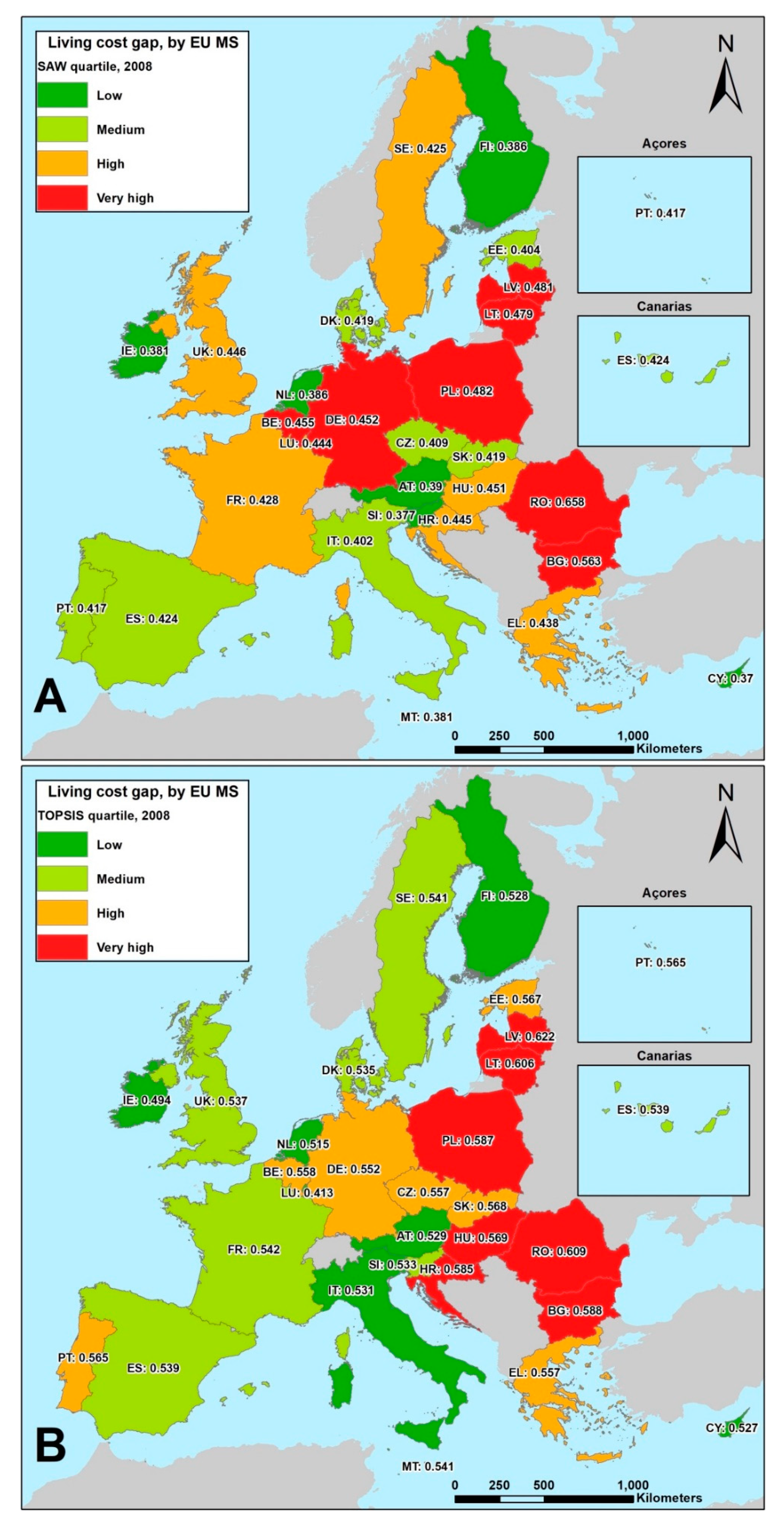
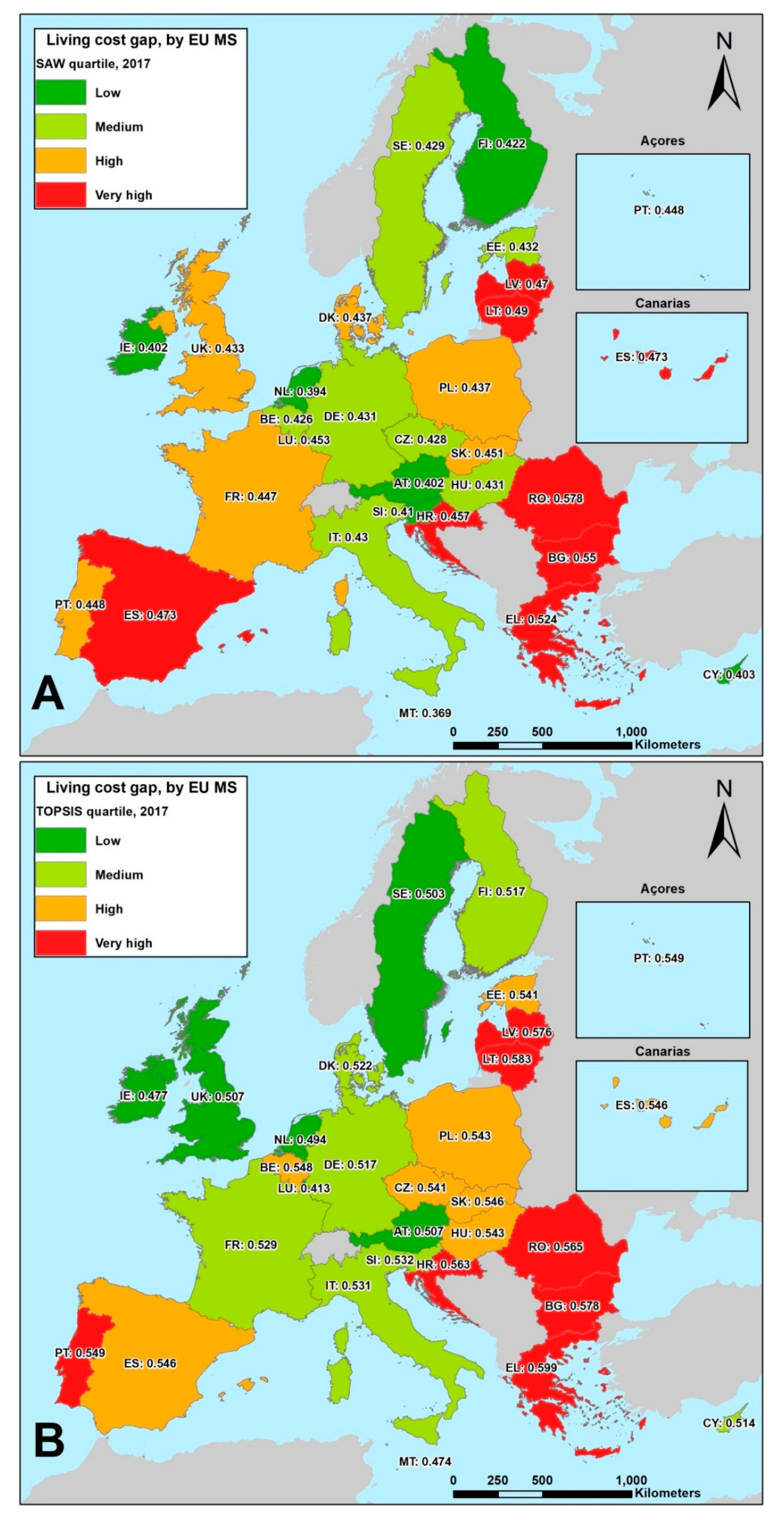
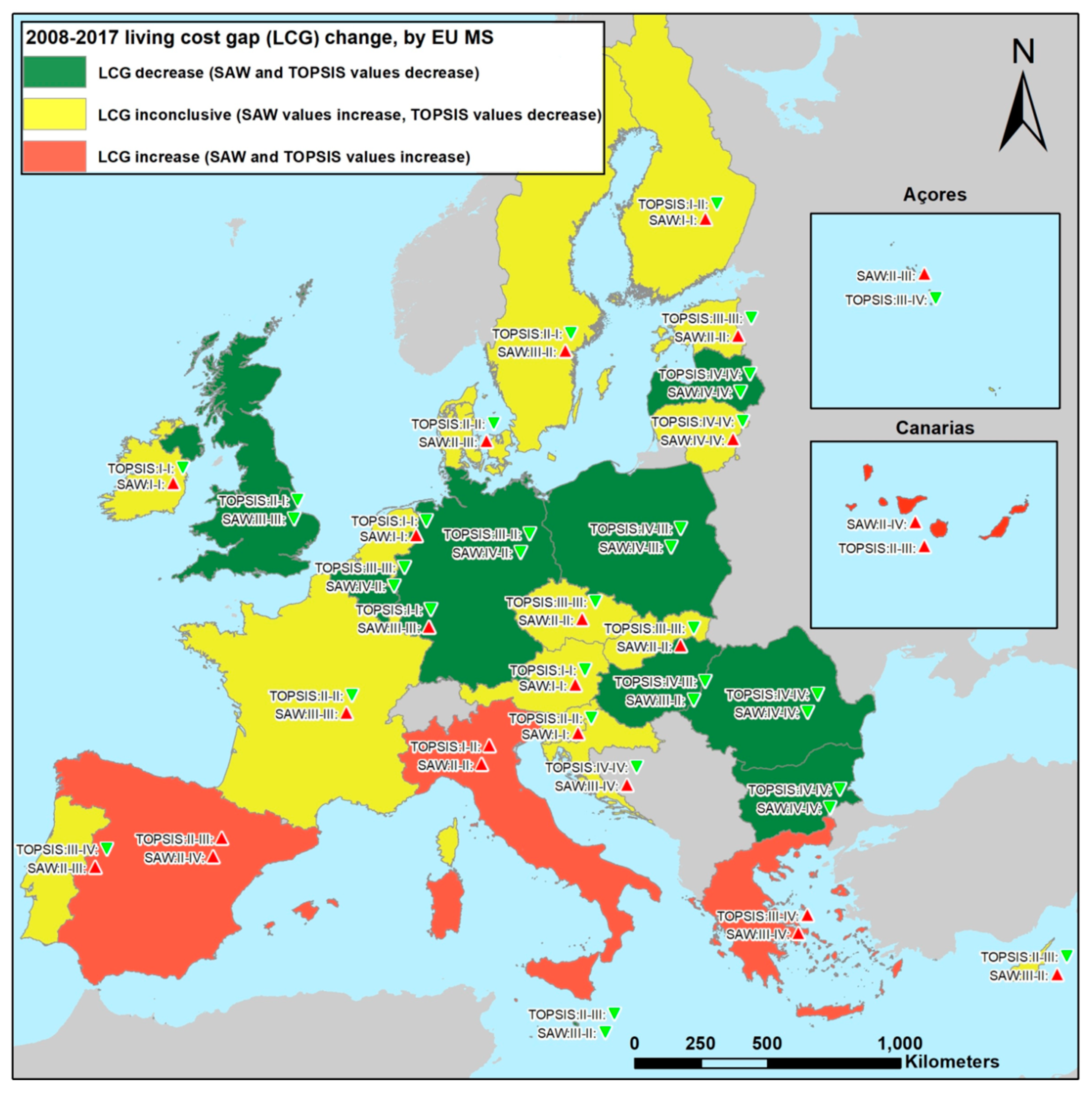
LCG and LCG Change Trends
- Estonia was more similar to Finland, rather than to the other two Baltic States;
- The situation in the Benelux area was very diverse;
- Czechia and Slovakia were rather similar;
- The Southern layer of the EU, which in other contexts is often put together and demonstrates similarities, was very distinct.
4. Discussion
4.1. Possible Framework Advantages and Drawbacks
4.2. Criteria Importance Definition and Assessment
4.3. Detailed Analysis of Changes in LCG
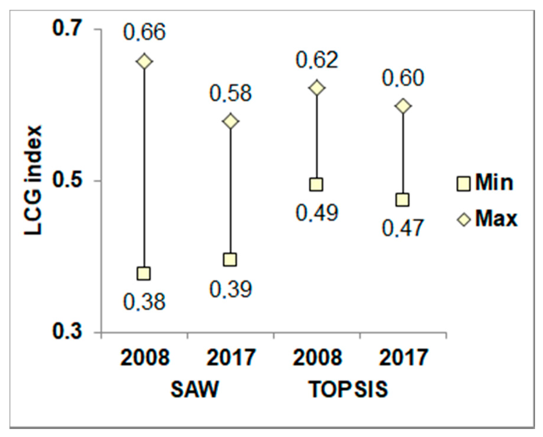
- With one single exception (the maximum value for 2017), the SAW method tended to generate lower minimum value and higher maximum values than the TOPSIS method. As a result, the gap between minimum and maximum values under the SAW method was constantly larger than the one under the TOPSIS method.
- Under both methods, the gap between minimum and maximum values got smaller in 2017 compared to 2008. This means that the LCG divergence across the EU decreased, i.e., some kind of pan-EU LCG convergence occurred. Under the SAW method, the convergence was due to a significant decrease in the maximum LCG value, which compensated for the slight increase in the minimum LCG value. Under the TOPSIS method, the shrinking gap was due to a parallel moderate decline in both minimum and maximum LCG values.
4.4. The LCG Roots
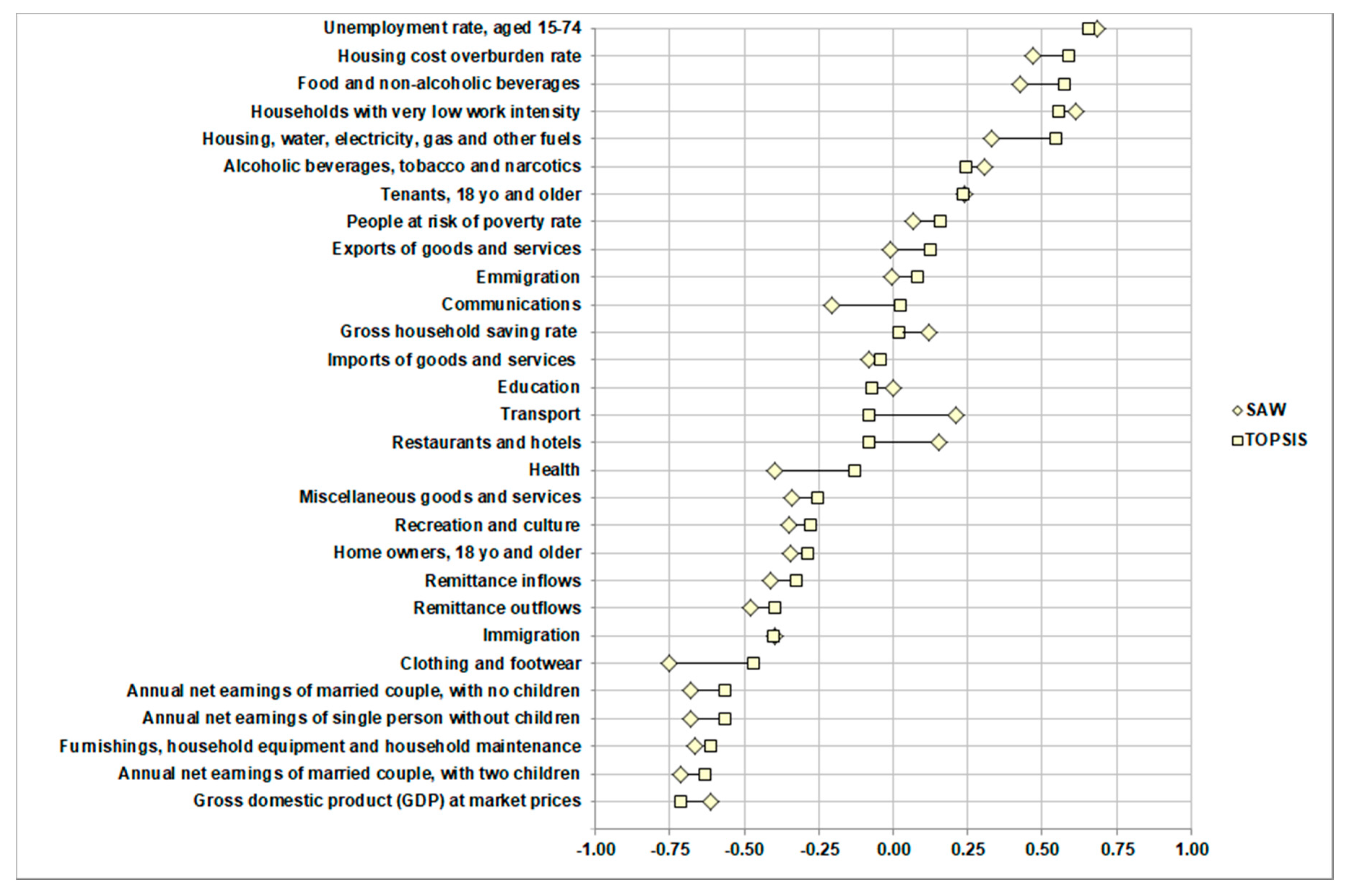
4.5. LCG Drivers
- With strong positive relationship: unemployment and low work intensity;
- With moderate positive relationship: housing cost overburden and basic household expenditures, i.e., food, housing;
- With weak positive relationship: house tenants, risk of income poverty, exports, and optional household expenditures (alcoholic beverages, tobacco).
- With strong negative relationship: GDP (in line with [66]), all types of net household earnings, household expenditure on optional needs (furnishing and clothing);
- With moderate negative relationship: immigration, remittance flows, home ownership, optional household expenditures (recreation and miscellaneous);
- With weak negative relationship: household savings, imports, optional household expenditures (communications, education, transport, restaurants, and health).
4.6. LCG and Housing
5. Conclusions
Author Contributions
Funding
Acknowledgments
Conflicts of Interest
Disclaimer
Appendix A

| No. | Indicator/Criterion Name 1 | Unit of Measure | Brief Description |
|---|---|---|---|
| 1. | Food and non-alcoholic beverages | Percentage of total household expenditure | Household expenditure refers to any spending done by a person living alone or by a group of people living together in shared accommodation and with common domestic expenses. It includes expenditure incurred on the domestic territory (by residents and non-residents) for the direct satisfaction of individual needs and covers the purchase of goods and services, the consumption of own production (such as garden produce) and the imputed rent of owner-occupied dwellings [41]. |
| 2. | Alcoholic beverages, tobacco, and narcotics | ||
| 3. | Clothing and footwear | ||
| 4. | Housing, water, electricity, gas, and other fuels | ||
| 5. | Furnishings, household equipment and routine household maintenance | ||
| 6. | Health | ||
| 7. | Transport | ||
| 8. | Communications | ||
| 9. | Recreation and culture | ||
| 10. | Education | ||
| 11. | Restaurants and hotels | ||
| 12. | Miscellaneous goods and services | ||
| 13. | Household savings | Saving percentage per household | The gross saving rate of households (including Non-Profit Institutions Serving Households) is defined as gross saving divided by gross disposable income, with the latter being adjusted for the change in the net equity of households in pension funds reserves. Gross saving is the part of the gross disposable income which is not spent as final consumption expenditure [42]. |
| 14. | Annual net earnings of single person without children | Total EUR per capita | Information on net earnings (net pay taken home, in absolute figures) and related tax-benefit rates (in%) complements gross-earnings data with respect to disposable earnings. The transition from gross to net earnings requires the deduction of income taxes and employee’s social security contributions from the gross amounts and the addition of family allowances, if appropriate [43]. |
| 15. | Annual net earnings of married couple with no children | Total EUR per household | |
| 16. | Annual net earnings of married couple with two children | ||
| 17. | Housing cost overburden rate | Percentage of total population | Percentage of the population living in a household where total housing costs (net of housing allowances) represent more than 40% of the total disposable household income (net of housing allowances) [44]. |
| 18. | Tenants, 18 yo and older | Percentage of total population | Distribution of population by a broad group of citizenship and tenure status (population aged 18 and over) [45]. |
| 19. | Homeowners, 18 yo and older | ||
| 20. | Unemployment rate, aged 15–74 | Percentage of active population | The unemployment rate is the number of unemployed persons as a percentage of the labour force based on International Labour Office (ILO) definition. The labour force is the total number of people employed and unemployed. Unemployed persons comprise persons aged 15 to 74 who are without work during the reference week, are available to start work within the next two weeks, and have been actively seeking work in the past four weeks or had already found a job to start within the next three months [46]. |
| 21. | Gross domestic product (GDP) at market prices | Total EUR per capita | The indicator is calculated as the ratio of real GDP to the average population of a specific year. GDP measures the value of total final output of goods and services produced by an economy within a certain period of time. It includes goods and services that have markets (or which could have markets) and products which are produced by general government and non-profit institutions. It is a measure of economic activity and is also used as a proxy for the development in a country’s material living standards. However, it is a limited measure of economic welfare. For example, GDP does not include most unpaid household work nor does GDP take account of negative effects of economic activity, like environmental degradation [47]. |
| 22. | Households with very low work intensity | Percentage of total population | People living in households with very low work intensity are people aged 0–59 living in households where the adults work 20% or less of their total work potential during the past year [48]. |
| 23. | People at risk of poverty rate | Percentage of total population | People at risk-of-poverty are persons with an equivalised disposable income below the risk-of-poverty threshold, which is set at 60% of the national median equivalised disposable income (after social transfers). The indicator is part of the multidimensional poverty index [49]. |
| 24. | Remittance inflows 1 | Total USD per capita | World Bank staff calculation based on data from IMF Balance of Payments Statistics database and data releases from central banks, national statistical agencies, and World Bank country desks [54]. |
| 25. | Remittance outflows 1 | ||
| 26. | Emigration | Percentage of total population | Total number of long-term emigrants leaving from the reporting country during the reference year [50]. |
| 27. | Immigration | Total number of long-term immigrants arriving into the reporting country during the reference year [51]. | |
| 28. | Exports of goods and services | Percentage of GDP | This indicator is the value of exports of goods and services divided by the GDP in current prices [52]. |
| 29. | Imports of goods and services | This indicator is the value of imports of goods and services divided by the GDP in current prices [53]. |
| Criterion No. 1 | Objective Function Group | Objective Function (Focusing on Highest LCG) Explanation | Objective Function Defined |
|---|---|---|---|
| 1 | ii. Adjacent–Micro–Local–Individual | Household expenditure on food (basic needs) is the highest. | MAX |
| 2 | iii. Adjacent–Micro–Local–Individual | Household expenditure on alcoholic beverages (optional needs) is the lowest. | MIN |
| 3 | iii. Adjacent–Micro–Local–Individual | Household expenditure on clothing (optional needs) is the lowest. | MIN |
| 4 | ii. Adjacent–Micro–Local–Individual | Household expenditure on housing (basic needs) is the highest. | MAX |
| 5 | iii. Adjacent–Micro–Local–Individual | Household expenditure on furniture (optional needs) is the lowest. | MIN |
| 6 | iii. Adjacent–Micro–Local–Individual | Household expenditure on health (optional needs) is the lowest. | MIN |
| 7 | ii. Adjacent–Micro–Local–Individual | Household expenditure on transport (basic needs) is the highest. | MAX |
| 8 | iii. Adjacent–Micro–Local–Individual | Household expenditure on communications (optional needs) is the lowest. | MIN |
| 9 | iii. Adjacent–Micro–Local–Individual | Household expenditure on recreation (optional needs) is the lowest. | MIN |
| 10 | iii. Adjacent–Micro–Local–Individual | Household expenditure on education (optional needs) is the lowest. | MIN |
| 11 | iii. Adjacent–Micro–Local–Individual | Household expenditure on restaurants (optional needs) is the lowest. | MIN |
| 12 | iii. Adjacent–Micro–Local–Individual | Household expenditure on miscellaneous goods (optional needs) is the lowest. | MIN |
| 13 | i. Adjacent–Micro–Local–Individual | Household savings are the lowest. Smallest savings means that most of income is spent on basic needs. This is the major driver of economic emigration. | MIN |
| 14 | i. Adjacent–Micro–Local–Individual | Single person income is the smallest. Smallest net income means that less money for optional expenditures and savings. | MIN |
| 15 | i. Adjacent–Micro–Local–Individual | Family without children income is the smallest. Smallest net income means that less money for optional expenditures and savings. | MIN |
| 16 | i. Adjacent–Micro–Local–Individual | Family with children income is the smallest. Smallest net income means that less money for optional expenditures and savings. | MIN |
| 17 | v. Neighboring–Mezo–National–External | Household cost overburden rate is highest. Means that less money households can allocate for optional expenditures and savings. | MAX |
| 18 | v. Neighboring–Mezo–National–External | Tenant ratio is the highest. Means competition for the housing is higher. It also means that less money households can allocate for optional expenditures and savings. | MAX |
| 19 | v. Neighboring–Mezo–National–External | Homeowner ratio is the smallest. Means competition for the housing is smaller. It also means that more money households can allocate for optional expenditures and savings. | MIN |
| 20 | iv. Neighboring–Mezo–National–External | Unemployment rate is the highest. Means that competition for workplaces is high. It also means that household receive less income and have to allocate larger share of income for basic needs. | MAX |
| 21 | iv. Neighboring–Mezo–National–External | GDP is lowest. Low GDP show low country economic performance. It means that more money households have to spend on basic needs. | MIN |
| 22 | iv. Neighboring–Mezo–National–External | The low work intensity is the highest. It also means lower income for the households. | MAX |
| 23 | iv. Neighboring–Mezo–National–External | The highest number of population within the income poverty. It means that largest share of household income is allocated only for the basic needs. | MAX |
| 24 | vi. Distant–Macro–International–External | The remittance inflows are highest. It also shows that economic and employment situation in the country is tough because incoming remittances are used to support basic local household needs. | MAX |
| 25 | vi. Distant–Macro–International–External | The remittance outflows are lowest. It also shows that economic and employment situation in the country is tough because the low outgoing remittances show that there is no possibility to earn decent savings. | MIN |
| 26 | vi. Distant–Macro–International–External | The emigration is the highest. It shows that most of household income share are allocated for the basic needs. | MAX |
| 27 | vi. Distant–Macro–International–External | The immigration is the lowest. It shows that economic situation in country is tough and immigrants (especially economic ones) cannot earn decent income and savings. | MIN |
| 28 | vi. Distant–Macro–International–External | The export is the lowest. No production, no export of goods, no import of money. It also means that households in such country have to allocate more money for basic needs because of lower income. | MIN |
| 29 | vi. Distant–Macro–International–External | The import is the highest. No production, so import of goods and export of money. It also means that households in such country have to allocate more money for basic needs because of lower income. | MAX |
| Criterion No. (Table A1) | Year | Objective Function Applied 1 | |||||||||
|---|---|---|---|---|---|---|---|---|---|---|---|
| 2008 | 2009 | 2010 | 2011 | 2012 | 2013 | 2014 | 2015 | 2016 | 2017 | ||
| 1 | 0.034 | 0.034 | 0.034 | 0.034 | 0.034 | 0.034 | 0.034 | 0.034 | 0.034 | 0.034 | MAX |
| 2 | 0.034 | 0.034 | 0.034 | 0.034 | 0.034 | 0.034 | 0.034 | 0.034 | 0.034 | 0.034 | MIN |
| 3 | 0.034 | 0.034 | 0.034 | 0.034 | 0.034 | 0.034 | 0.034 | 0.034 | 0.034 | 0.034 | MIN |
| 4 | 0.034 | 0.034 | 0.034 | 0.034 | 0.034 | 0.034 | 0.034 | 0.034 | 0.034 | 0.034 | MAX |
| 5 | 0.034 | 0.034 | 0.034 | 0.034 | 0.034 | 0.034 | 0.034 | 0.034 | 0.034 | 0.034 | MIN |
| 6 | 0.035 | 0.035 | 0.034 | 0.035 | 0.034 | 0.034 | 0.034 | 0.034 | 0.034 | 0.034 | MIN |
| 7 | 0.034 | 0.034 | 0.034 | 0.034 | 0.034 | 0.034 | 0.034 | 0.034 | 0.034 | 0.034 | MAX |
| 8 | 0.034 | 0.034 | 0.034 | 0.034 | 0.034 | 0.034 | 0.034 | 0.034 | 0.034 | 0.034 | MIN |
| 9 | 0.034 | 0.034 | 0.034 | 0.034 | 0.034 | 0.034 | 0.034 | 0.034 | 0.034 | 0.034 | MIN |
| 10 | 0.035 | 0.035 | 0.035 | 0.035 | 0.035 | 0.035 | 0.035 | 0.035 | 0.035 | 0.035 | MIN |
| 11 | 0.035 | 0.034 | 0.035 | 0.035 | 0.035 | 0.035 | 0.035 | 0.034 | 0.035 | 0.035 | MIN |
| 12 | 0.035 | 0.035 | 0.034 | 0.034 | 0.034 | 0.034 | 0.034 | 0.035 | 0.035 | 0.035 | MIN |
| 13 | 0.036 | 0.036 | 0.036 | 0.036 | 0.036 | 0.036 | 0.036 | 0.036 | 0.036 | 0.036 | MIN |
| 14 | 0.035 | 0.035 | 0.035 | 0.035 | 0.035 | 0.035 | 0.035 | 0.035 | 0.035 | 0.035 | MIN |
| 15 | 0.035 | 0.035 | 0.035 | 0.035 | 0.035 | 0.035 | 0.035 | 0.035 | 0.035 | 0.035 | MIN |
| 16 | 0.035 | 0.035 | 0.035 | 0.035 | 0.035 | 0.035 | 0.035 | 0.035 | 0.035 | 0.035 | MIN |
| 17 | 0.034 | 0.035 | 0.034 | 0.035 | 0.035 | 0.035 | 0.035 | 0.035 | 0.035 | 0.035 | MAX |
| 18 | 0.034 | 0.034 | 0.034 | 0.034 | 0.034 | 0.034 | 0.034 | 0.034 | 0.034 | 0.034 | MAX |
| 19 | 0.034 | 0.034 | 0.034 | 0.034 | 0.034 | 0.034 | 0.034 | 0.034 | 0.034 | 0.034 | MIN |
| 20 | 0.034 | 0.034 | 0.034 | 0.034 | 0.035 | 0.035 | 0.035 | 0.035 | 0.035 | 0.035 | MAX |
| 21 | 0.035 | 0.035 | 0.035 | 0.035 | 0.035 | 0.035 | 0.035 | 0.035 | 0.035 | 0.035 | MIN |
| 22 | 0.034 | 0.034 | 0.034 | 0.035 | 0.034 | 0.034 | 0.034 | 0.034 | 0.034 | 0.034 | MAX |
| 23 | 0.034 | 0.034 | 0.034 | 0.034 | 0.034 | 0.034 | 0.034 | 0.034 | 0.034 | 0.034 | MAX |
| 24 | 0.035 | 0.035 | 0.035 | 0.035 | 0.035 | 0.035 | 0.035 | 0.035 | 0.035 | 0.035 | MAX |
| 25 | 0.035 | 0.035 | 0.035 | 0.035 | 0.035 | 0.035 | 0.035 | 0.035 | 0.035 | 0.035 | MIN |
| 26 | 0.035 | 0.035 | 0.035 | 0.035 | 0.035 | 0.035 | 0.035 | 0.035 | 0.035 | 0.035 | MAX |
| 27 | 0.036 | 0.036 | 0.036 | 0.036 | 0.035 | 0.035 | 0.035 | 0.035 | 0.035 | 0.035 | MIN |
| 28 | 0.034 | 0.034 | 0.034 | 0.034 | 0.034 | 0.034 | 0.034 | 0.034 | 0.034 | 0.034 | MIN |
| 29 | 0.035 | 0.035 | 0.035 | 0.035 | 0.035 | 0.035 | 0.035 | 0.035 | 0.035 | 0.035 | MAX |
| MS | Year | CAGR | |||||||||
|---|---|---|---|---|---|---|---|---|---|---|---|
| 2008 | 2009 | 2010 | 2011 | 2012 | 2013 | 2014 | 2015 | 2016 | 2017 | ||
| Belgium | 0.455 | 0.428 | 0.410 | 0.415 | 0.410 | 0.410 | 0.411 | 0.414 | 0.423 | 0.426 | −0.725 |
| Bulgaria | 0.563 | 0.535 | 0.562 | 0.569 | 0.550 | 0.544 | 0.543 | 0.548 | 0.552 | 0.550 | −0.256 |
| Czechia | 0.409 | 0.398 | 0.406 | 0.404 | 0.409 | 0.422 | 0.428 | 0.430 | 0.427 | 0.428 | 0.521 |
| Denmark | 0.419 | 0.421 | 0.430 | 0.419 | 0.413 | 0.421 | 0.422 | 0.422 | 0.430 | 0.437 | 0.466 |
| Germany | 0.452 | 0.425 | 0.422 | 0.419 | 0.412 | 0.414 | 0.415 | 0.416 | 0.428 | 0.431 | −0.532 |
| Estonia | 0.404 | 0.414 | 0.437 | 0.438 | 0.440 | 0.435 | 0.435 | 0.429 | 0.431 | 0.432 | 0.770 |
| Ireland | 0.381 | 0.383 | 0.399 | 0.418 | 0.411 | 0.401 | 0.402 | 0.396 | 0.404 | 0.402 | 0.590 |
| Greece | 0.438 | 0.414 | 0.429 | 0.468 | 0.497 | 0.503 | 0.508 | 0.513 | 0.521 | 0.524 | 2.004 |
| Spain | 0.424 | 0.416 | 0.437 | 0.449 | 0.458 | 0.473 | 0.475 | 0.473 | 0.471 | 0.473 | 1.231 |
| France | 0.428 | 0.414 | 0.424 | 0.423 | 0.425 | 0.428 | 0.428 | 0.433 | 0.440 | 0.447 | 0.464 |
| Croatia | 0.445 | 0.424 | 0.434 | 0.424 | 0.438 | 0.441 | 0.449 | 0.452 | 0.452 | 0.457 | 0.302 |
| Italy | 0.402 | 0.383 | 0.393 | 0.391 | 0.396 | 0.406 | 0.412 | 0.413 | 0.426 | 0.430 | 0.748 |
| Cyprus | 0.370 | 0.352 | 0.364 | 0.360 | 0.394 | 0.402 | 0.402 | 0.398 | 0.398 | 0.403 | 0.979 |
| Latvia | 0.481 | 0.495 | 0.505 | 0.506 | 0.493 | 0.478 | 0.467 | 0.465 | 0.469 | 0.470 | −0.268 |
| Lithuania | 0.479 | 0.482 | 0.525 | 0.518 | 0.486 | 0.485 | 0.477 | 0.488 | 0.490 | 0.490 | 0.275 |
| Luxembourg | 0.444 | 0.430 | 0.426 | 0.430 | 0.428 | 0.429 | 0.433 | 0.435 | 0.441 | 0.453 | 0.220 |
| Hungary | 0.451 | 0.428 | 0.434 | 0.439 | 0.446 | 0.450 | 0.442 | 0.433 | 0.432 | 0.431 | −0.501 |
| Malta | 0.381 | 0.376 | 0.375 | 0.373 | 0.362 | 0.368 | 0.365 | 0.368 | 0.373 | 0.369 | −0.372 |
| Netherlands | 0.386 | 0.377 | 0.385 | 0.386 | 0.381 | 0.386 | 0.388 | 0.392 | 0.391 | 0.394 | 0.219 |
| Austria | 0.390 | 0.379 | 0.385 | 0.393 | 0.385 | 0.387 | 0.386 | 0.387 | 0.395 | 0.402 | 0.358 |
| Poland | 0.482 | 0.464 | 0.455 | 0.451 | 0.442 | 0.442 | 0.440 | 0.445 | 0.447 | 0.437 | −1.095 |
| Portugal | 0.417 | 0.393 | 0.405 | 0.410 | 0.440 | 0.447 | 0.453 | 0.453 | 0.450 | 0.448 | 0.790 |
| Romania | 0.658 | 0.633 | 0.600 | 0.607 | 0.612 | 0.580 | 0.582 | 0.581 | 0.585 | 0.578 | −1.421 |
| Slovenia | 0.377 | 0.369 | 0.377 | 0.379 | 0.383 | 0.395 | 0.397 | 0.403 | 0.408 | 0.410 | 0.939 |
| Slovakia | 0.419 | 0.403 | 0.418 | 0.418 | 0.439 | 0.446 | 0.445 | 0.447 | 0.450 | 0.451 | 0.824 |
| Finland | 0.386 | 0.377 | 0.384 | 0.385 | 0.387 | 0.393 | 0.401 | 0.409 | 0.417 | 0.422 | 0.987 |
| Sweden | 0.425 | 0.417 | 0.419 | 0.421 | 0.411 | 0.416 | 0.414 | 0.418 | 0.424 | 0.429 | 0.112 |
| United Kingdom | 0.446 | 0.430 | 0.433 | 0.427 | 0.417 | 0.421 | 0.423 | 0.423 | 0.432 | 0.433 | −0.323 |
| MS | Year | CAGR | |||||||||
|---|---|---|---|---|---|---|---|---|---|---|---|
| 2008 | 2009 | 2010 | 2011 | 2012 | 2013 | 2014 | 2015 | 2016 | 2017 | ||
| Belgium | 0.558 | 0.551 | 0.548 | 0.559 | 0.552 | 0.539 | 0.535 | 0.536 | 0.541 | 0.548 | −0.216 |
| Bulgaria | 0.588 | 0.567 | 0.570 | 0.582 | 0.581 | 0.569 | 0.561 | 0.568 | 0.572 | 0.578 | −0.206 |
| Czechia | 0.557 | 0.545 | 0.554 | 0.562 | 0.550 | 0.538 | 0.533 | 0.536 | 0.534 | 0.541 | −0.327 |
| Denmark | 0.535 | 0.530 | 0.532 | 0.536 | 0.529 | 0.517 | 0.515 | 0.510 | 0.512 | 0.522 | −0.275 |
| Germany | 0.552 | 0.538 | 0.534 | 0.539 | 0.527 | 0.513 | 0.506 | 0.502 | 0.511 | 0.517 | −0.718 |
| Estonia | 0.567 | 0.555 | 0.571 | 0.581 | 0.569 | 0.553 | 0.542 | 0.540 | 0.541 | 0.541 | −0.514 |
| Ireland | 0.494 | 0.490 | 0.499 | 0.519 | 0.504 | 0.491 | 0.485 | 0.475 | 0.474 | 0.477 | −0.409 |
| Greece | 0.557 | 0.541 | 0.544 | 0.575 | 0.589 | 0.586 | 0.591 | 0.598 | 0.593 | 0.599 | 0.822 |
| Spain | 0.539 | 0.537 | 0.546 | 0.556 | 0.556 | 0.549 | 0.542 | 0.542 | 0.540 | 0.546 | 0.140 |
| France | 0.542 | 0.531 | 0.538 | 0.544 | 0.531 | 0.519 | 0.515 | 0.521 | 0.522 | 0.529 | −0.265 |
| Croatia | 0.585 | 0.572 | 0.572 | 0.575 | 0.564 | 0.553 | 0.549 | 0.555 | 0.555 | 0.563 | −0.413 |
| Italy | 0.531 | 0.520 | 0.526 | 0.536 | 0.530 | 0.519 | 0.515 | 0.520 | 0.525 | 0.531 | 0.012 |
| Cyprus | 0.527 | 0.480 | 0.502 | 0.501 | 0.529 | 0.539 | 0.535 | 0.519 | 0.512 | 0.514 | −0.274 |
| Latvia | 0.622 | 0.607 | 0.621 | 0.628 | 0.613 | 0.591 | 0.577 | 0.577 | 0.571 | 0.576 | −0.853 |
| Lithuania | 0.606 | 0.593 | 0.631 | 0.630 | 0.599 | 0.588 | 0.577 | 0.578 | 0.576 | 0.583 | −0.426 |
| Luxembourg | 0.413 | 0.417 | 0.407 | 0.403 | 0.400 | 0.396 | 0.397 | 0.404 | 0.411 | 0.413 | −0.025 |
| Hungary | 0.569 | 0.553 | 0.558 | 0.572 | 0.568 | 0.553 | 0.541 | 0.537 | 0.535 | 0.543 | −0.519 |
| Malta | 0.541 | 0.514 | 0.527 | 0.531 | 0.503 | 0.487 | 0.475 | 0.480 | 0.482 | 0.474 | −1.463 |
| Netherlands | 0.515 | 0.505 | 0.513 | 0.519 | 0.510 | 0.502 | 0.496 | 0.498 | 0.488 | 0.494 | −0.459 |
| Austria | 0.529 | 0.518 | 0.522 | 0.528 | 0.511 | 0.499 | 0.492 | 0.491 | 0.496 | 0.507 | −0.462 |
| Poland | 0.587 | 0.572 | 0.572 | 0.582 | 0.569 | 0.554 | 0.547 | 0.545 | 0.541 | 0.543 | −0.855 |
| Portugal | 0.565 | 0.543 | 0.550 | 0.565 | 0.561 | 0.552 | 0.548 | 0.550 | 0.546 | 0.549 | −0.324 |
| Romania | 0.609 | 0.584 | 0.573 | 0.571 | 0.569 | 0.561 | 0.557 | 0.559 | 0.558 | 0.565 | −0.842 |
| Slovenia | 0.533 | 0.524 | 0.543 | 0.552 | 0.540 | 0.529 | 0.525 | 0.527 | 0.527 | 0.532 | −0.012 |
| Slovakia | 0.568 | 0.558 | 0.560 | 0.570 | 0.559 | 0.545 | 0.541 | 0.543 | 0.541 | 0.546 | −0.428 |
| Finland | 0.528 | 0.516 | 0.522 | 0.528 | 0.517 | 0.505 | 0.504 | 0.509 | 0.510 | 0.517 | −0.225 |
| Sweden | 0.541 | 0.531 | 0.528 | 0.533 | 0.515 | 0.501 | 0.495 | 0.500 | 0.494 | 0.503 | −0.787 |
| United Kingdom | 0.537 | 0.523 | 0.521 | 0.531 | 0.510 | 0.500 | 0.495 | 0.492 | 0.498 | 0.507 | −0.639 |
| MS | Criterion Number (Table A1) | ||||||||||||||||||||||||||||
|---|---|---|---|---|---|---|---|---|---|---|---|---|---|---|---|---|---|---|---|---|---|---|---|---|---|---|---|---|---|
| 1 | 2 | 3 | 4 | 5 | 6 | 7 | 8 | 9 | 10 | 11 | 12 | 13 | 14 | 15 | 16 | 17 | 18 | 19 | 20 | 21 | 22 | 23 | 24 | 25 | 26 | 27 | 28 | 29 | |
| Belgium | 0.518 | 0.557 | 0.464 | 0.723 | 0.000 | 1.048 | −1.223 | −0.962 | −1.389 | 0.000 | 1.317 | −0.983 | −4.414 | 1.672 | 1.688 | 1.620 | −3.466 | −0.735 | 0.235 | 0.371 | 0.521 | 1.603 | 0.876 | −0.656 | 0.497 | 3.790 | −1.582 | 0.191 | 0.097 |
| Bulgaria | −0.671 | −3.249 | −0.341 | 1.332 | −2.873 | 4.889 | −1.413 | −1.300 | −0.141 | 3.602 | 2.347 | 1.918 | 0.000 | 6.342 | 6.342 | 5.562 | 3.982 | 3.026 | −0.461 | 1.663 | 2.305 | 3.563 | 0.998 | 2.204 | 2.959 | 14.423 | 13.368 | 2.798 | −1.518 |
| Czechia | 1.231 | 1.178 | −0.296 | 0.044 | −0.805 | −1.300 | 0.336 | −2.205 | −1.381 | −3.670 | 1.896 | −1.739 | −1.986 | 2.442 | 2.442 | 2.428 | −4.200 | −0.940 | 0.254 | −4.405 | 1.214 | −2.948 | 0.123 | 13.369 | −2.739 | −7.031 | −8.086 | 2.611 | 1.872 |
| Denmark | 0.195 | −0.616 | −0.782 | 0.897 | −0.411 | 0.405 | −0.633 | −0.541 | −0.188 | 1.495 | 0.955 | −1.258 | 11.441 | 1.550 | 1.550 | 1.533 | −0.945 | 0.961 | −0.565 | 6.800 | 0.397 | 1.822 | 0.553 | 2.265 | −3.495 | 3.815 | 1.455 | 0.183 | −0.583 |
| Germany | −0.103 | −0.341 | −0.903 | −0.677 | 0.526 | 0.893 | 0.332 | −2.162 | 0.518 | 1.317 | 0.859 | 0.359 | 0.213 | 2.405 | 2.405 | 2.373 | 0.000 | 0.278 | −0.257 | −7.710 | 1.023 | −3.238 | 0.641 | 4.787 | 4.176 | −3.045 | 3.301 | 0.882 | 0.744 |
| Estonia | 0.112 | 0.720 | 0.170 | 0.434 | −1.215 | 1.495 | −1.088 | −4.546 | 0.268 | −5.088 | 2.716 | −1.041 | 4.914 | 5.234 | 5.234 | 5.355 | 3.248 | 3.083 | −0.582 | 1.372 | 1.490 | 1.007 | 0.827 | 3.825 | 5.119 | 12.356 | 19.264 | 1.544 | 0.266 |
| Ireland | −0.364 | −1.393 | −1.331 | 0.634 | −3.634 | 4.272 | 0.433 | −2.362 | −1.565 | 0.455 | 2.684 | −2.273 | 0.258 | 0.515 | 0.515 | 0.389 | 3.506 | 1.798 | −0.444 | 0.812 | 3.852 | 1.880 | 0.071 | −1.057 | −6.282 | −1.099 | −1.341 | 4.125 | 3.057 |
| Greece | 1.259 | 2.281 | −3.711 | 0.697 | −7.038 | −0.962 | −1.300 | 2.255 | −0.239 | −1.473 | 2.076 | −1.283 | 0.000 | −1.945 | −1.922 | −2.790 | 6.642 | 1.539 | −0.390 | 13.234 | −2.838 | 8.478 | 0.055 | −21.135 | −7.972 | 10.548 | 6.300 | 3.894 | −0.633 |
| Spain | −0.267 | 0.000 | −1.594 | 1.126 | −1.117 | 1.495 | 0.272 | −0.851 | −0.576 | 2.334 | −0.294 | −0.885 | −3.578 | 0.868 | 0.868 | 0.859 | 0.464 | 2.527 | −0.460 | 5.496 | 0.096 | 7.637 | 0.971 | 0.766 | −8.885 | 2.558 | −1.512 | 3.602 | 0.431 |
| France | 0.514 | 0.944 | −1.364 | 0.748 | −0.658 | 0.000 | −0.242 | −3.146 | −1.192 | 2.510 | 1.298 | −0.692 | −0.803 | 1.165 | 1.165 | 1.159 | 1.956 | −0.618 | 0.321 | 3.201 | 0.371 | −0.917 | 0.607 | 1.924 | −0.280 | 2.500 | 2.000 | 1.025 | 0.949 |
| Croatia | −0.234 | 0.879 | −1.698 | 0.400 | −0.942 | −1.029 | −1.784 | 0.572 | 0.676 | 4.043 | 1.561 | −0.851 | 5.464 | 1.311 | 1.311 | 1.853 | −9.399 | −2.449 | 0.245 | 3.495 | 0.087 | −1.439 | −0.328 | 2.495 | 1.879 | 18.536 | −0.496 | 3.590 | 0.650 |
| Italy | −0.155 | 0.000 | −0.885 | 0.922 | −1.021 | 1.001 | −0.516 | −1.698 | −0.326 | 1.178 | 1.386 | −0.835 | −3.392 | 1.034 | 1.034 | 1.030 | −0.135 | −0.794 | 0.229 | 6.294 | −0.700 | 1.413 | 0.797 | 2.879 | −5.056 | 7.106 | −5.143 | 1.516 | 0.120 |
| Cyprus | −0.274 | 0.603 | −1.034 | −1.081 | −1.966 | 2.350 | −1.509 | −1.577 | 0.526 | 3.117 | 2.644 | 0.129 | 0.625 | 0.001 | 0.001 | 0.001 | 5.032 | 0.000 | 0.000 | 13.771 | −0.723 | 8.529 | −0.141 | −11.375 | −1.918 | 13.258 | −0.936 | 4.271 | 1.748 |
| Latvia | −0.715 | 0.461 | 0.212 | −0.897 | 0.572 | 2.761 | 0.095 | −1.125 | 0.464 | 0.000 | 1.590 | 0.495 | −10.140 | 4.042 | 4.042 | 4.235 | −2.543 | 4.343 | −0.713 | 1.798 | 1.635 | 4.170 | −1.747 | −3.284 | −6.488 | −3.340 | 10.126 | 5.156 | 1.887 |
| Lithuania | −1.372 | −0.358 | −1.381 | 0.074 | 2.426 | −0.249 | −1.164 | 2.716 | 2.270 | −2.005 | 3.347 | 1.584 | 12.558 | 4.398 | 4.398 | 4.368 | 4.135 | 1.873 | −0.170 | 3.133 | 2.585 | 5.289 | 1.021 | −0.708 | −0.600 | 8.590 | 10.576 | 2.861 | 0.398 |
| Luxembourg | 0.365 | −0.398 | 0.650 | 1.101 | −1.300 | 5.963 | −2.030 | −0.764 | −0.178 | 0.000 | 0.153 | 0.000 | 2.032 | 1.694 | 1.677 | 1.540 | 11.681 | −1.431 | 0.233 | 2.334 | 0.091 | 4.359 | 3.772 | −1.522 | −1.070 | 1.331 | 1.312 | 1.692 | 1.730 |
| Hungary | 0.504 | 0.149 | 1.928 | −0.913 | −0.685 | 1.118 | −1.272 | −0.304 | −1.195 | 2.181 | 3.602 | −0.247 | 3.161 | 4.478 | 4.478 | 4.806 | −0.893 | 4.161 | −0.541 | −6.974 | 1.429 | −6.427 | 0.865 | 7.299 | −6.034 | 17.465 | 7.098 | 1.048 | 0.140 |
| Malta | −2.139 | −0.541 | −1.117 | −1.527 | −1.513 | −0.841 | −0.449 | −0.885 | −0.328 | 3.946 | 4.409 | 0.206 | 0.000 | 2.478 | 2.478 | 2.774 | −9.087 | −2.194 | 0.558 | −4.742 | 3.063 | −2.107 | 0.978 | −2.596 | −4.340 | 5.881 | 13.709 | 0.045 | −1.660 |
| Netherlands | 1.123 | 1.100 | 0.208 | 1.603 | −0.751 | 2.510 | −1.145 | −3.440 | −1.251 | 0.000 | 1.861 | −2.244 | 3.749 | 1.755 | 1.755 | 1.821 | −4.099 | −0.587 | 0.304 | 4.751 | 0.254 | 1.649 | 2.575 | 3.205 | −1.675 | 1.605 | 2.683 | 1.998 | 1.898 |
| Austria | −0.224 | −0.671 | −0.376 | 0.723 | −0.164 | 0.587 | −1.037 | −2.100 | 0.000 | 1.317 | 1.434 | −0.749 | −3.221 | 2.256 | 2.256 | 2.131 | −1.980 | 0.513 | −0.328 | 4.144 | 0.246 | 1.283 | −0.599 | −1.268 | 5.201 | 2.186 | 4.096 | 0.166 | 0.425 |
| Poland | −1.744 | −2.486 | 2.618 | −0.211 | 2.563 | 4.307 | 0.557 | −3.262 | 0.572 | −2.005 | 2.832 | 0.086 | −1.979 | 4.298 | 4.298 | 5.016 | −4.028 | −7.379 | 2.280 | −3.781 | 3.190 | −3.696 | −1.316 | −4.539 | 16.633 | 24.672 | 33.814 | 4.076 | 1.761 |
| Portugal | 0.477 | 0.365 | 0.181 | 1.932 | −2.449 | 0.662 | −0.955 | −2.449 | −1.809 | 0.000 | 2.644 | −2.490 | −0.702 | 0.696 | 0.696 | 0.775 | −1.391 | 0.139 | −0.044 | 0.729 | 0.249 | 2.690 | −0.121 | 0.703 | 0.052 | 5.337 | 2.620 | 3.511 | 0.243 |
| Romania | −0.617 | 2.046 | 1.994 | 0.350 | 0.812 | 5.778 | −3.755 | 7.120 | 2.732 | −3.886 | −5.252 | 0.587 | 0.000 | 6.009 | 6.009 | 5.978 | −4.772 | 0.770 | −0.023 | −1.079 | 2.385 | −2.291 | 0.000 | 11.450 | 9.526 | −1.916 | 3.319 | 5.243 | 1.247 |
| Slovenia | −0.077 | 0.220 | 0.000 | 0.294 | −1.666 | 0.918 | 0.412 | −1.473 | −1.032 | 0.000 | 0.759 | 0.113 | −2.295 | 1.644 | 1.644 | 1.797 | 1.873 | 2.453 | −0.527 | 5.903 | 0.138 | −0.858 | 0.872 | 2.256 | −5.897 | 3.897 | −5.583 | 2.555 | 0.924 |
| Slovakia | 0.676 | 1.728 | −1.506 | −0.787 | −0.872 | 3.717 | 0.337 | −1.300 | 0.810 | 1.495 | −1.238 | 0.904 | 2.514 | 2.427 | 2.427 | 2.342 | 4.608 | −0.811 | 0.086 | −1.677 | 1.933 | 0.420 | 1.443 | 0.469 | 8.585 | 8.070 | −2.299 | 1.926 | 1.410 |
| Finland | −0.554 | −0.700 | −1.473 | 2.110 | −1.531 | 0.971 | −0.900 | −0.885 | −1.758 | 0.000 | 0.000 | 0.000 | −0.595 | 1.396 | 1.396 | 1.324 | −0.983 | 1.053 | −0.398 | 4.207 | −0.320 | 4.027 | −1.846 | −2.475 | 2.614 | 2.018 | 0.564 | −1.923 | −1.037 |
| Sweden | 0.179 | −0.322 | −0.730 | −0.386 | 0.187 | 0.353 | 0.090 | 1.137 | −0.488 | 0.000 | 1.337 | 0.101 | 2.423 | 3.244 | 3.244 | 3.161 | −1.919 | −0.570 | 0.283 | 2.676 | 0.917 | 2.575 | 1.763 | −4.426 | 2.728 | −0.858 | 3.064 | −1.134 | −0.703 |
| United Kingdom | −0.281 | −1.300 | 0.437 | −0.042 | 0.495 | 3.451 | −0.406 | −1.228 | 0.305 | 5.361 | 0.234 | −0.832 | −5.363 | 2.059 | 2.059 | 2.012 | −2.993 | 1.958 | −0.755 | −2.174 | 0.534 | −0.325 | −1.053 | −4.116 | −2.301 | −2.623 | 0.227 | 1.327 | 0.920 |
| R1 (SAW) | 0.428 | 0.306 | −0.749 | 0.329 | −0.666 | −0.397 | 0.210 | −0.204 | −0.347 | 0.002 | 0.154 | −0.341 | 0.119 | −0.681 | −0.681 | −0.714 | 0.471 | 0.240 | −0.346 | 0.685 | −0.611 | 0.614 | 0.067 | −0.412 | −0.480 | −0.006 | −0.398 | −0.010 | −0.080 |
| R2 (TOPSIS) | 0.577 | 0.243 | −0.471 | 0.548 | −0.612 | −0.127 | −0.080 | 0.022 | −0.278 | −0.070 | −0.082 | −0.253 | 0.021 | −0.564 | −0.563 | −0.631 | 0.591 | 0.234 | −0.288 | 0.656 | −0.716 | 0.555 | 0.157 | −0.325 | −0.397 | 0.080 | −0.401 | 0.124 | −0.045 |


References
- Alesina, A.; Di Tella, R.; MacCulloch, R. Inequality and happiness: Are Europeans and Americans different? J. Public Econ. 2004, 88, 2009–2042. [Google Scholar] [CrossRef]
- Bettencourt, L.M.A.; Lobo, J.; Helbing, D.; Kuhnert, C.; West, G.B. Growth, innovation, scaling, and the pace of life in cities. Proc. Natl. Acad. Sci. USA 2007, 104, 7301–7306. [Google Scholar] [CrossRef]
- Charron, N.; Dijkstra, L.; Lapuente, V. Erratum to: Mapping the Regional Divide in Europe: A Measure for Assessing Quality of Government in 206 European Regions. Soc. Indic. Res. 2015, 124, 1059. [Google Scholar] [CrossRef]
- Glaeser, E.L.; Resseger, M.; Tobio, K. Inequality in cities. J. Reg. Sci. 2009, 49, 617–646. [Google Scholar] [CrossRef]
- Persson, T.; Tabellini, G. Is Inequality Harmful for Growth? Theory and Evidence. Natl. Bur. Econ. Res. 1991. [Google Scholar] [CrossRef]
- Reardon, S.F.; O’Sullivan, D. Measures of Spatial Segregation. Sociol. Methodol. 2004, 34, 121–162. [Google Scholar] [CrossRef]
- Norris, M.; Winston, N. Home-ownership, housing regimes and income inequalities in Western Europe. Int. J. Soc. Welf. 2012, 21, 127–138. [Google Scholar] [CrossRef]
- Vojnovic, I. Urban sustainability: Research, politics, policy and practice. Cities 2014, 41, S30–S44. [Google Scholar] [CrossRef]
- Dijkstra, L. My Region, My Europe, Our Future. Seventh Report on Economic, Social and Territorial Cohesion; Publications Office of the European Union: Luxembourg, 2017; ISBN 978-92-79-71834-2. [Google Scholar]
- Scholliers, P.; Schwarz, L.D. Experiencing Wages: Social and Cultural Aspects of Wage Forms in Europe since 1500; Berghahn Books: New York, NY, USA, 2003; Volume 4, ISBN 1-57181-546-5. [Google Scholar]
- Dijkstra, L.; Garcilazo, E.; McCann, P. The Economic Performance of European Cities and City Regions: Myths and Realities. Eur. Plan. Stud. 2013, 21, 334–354. [Google Scholar] [CrossRef]
- Quigley, J.M.; Raphael, S. Is Housing Unaffordable? Why Isn’t It More Affordable? J. Econ. Perspect. 2004, 18, 191–214. [Google Scholar] [CrossRef]
- Mimura, Y. Housing Cost Burden, Poverty Status, and Economic Hardship among Low-income Families. J. Fam. Econ. Issues 2008, 29, 152–165. [Google Scholar] [CrossRef]
- Saiz, A. Immigration and housing rents in American cities. J. Urban Econ. 2007, 61, 345–371. [Google Scholar] [CrossRef]
- McConnell, E.D.; Akresh, I.R. Housing Cost Burden and New Lawful Immigrants in the United States. Popul. Res. Policy Rev. 2010, 29, 143–171. [Google Scholar] [CrossRef]
- Dohmen, T.J. Housing, mobility and unemployment. Reg. Sci. Urban Econ. 2005, 35, 305–325. [Google Scholar] [CrossRef]
- Blanchard, O.; Katz, L.F. What We Know and Do Not Know About the Natural Rate of Unemployment. J. Econ. Perspect. 1997, 11, 51–72. [Google Scholar] [CrossRef]
- Arundel, R.; Lennartz, C. Housing market dualization: Linking insider–outsider divides in employment and housing outcoms. Hous. Stud. 2019, 1–25. [Google Scholar] [CrossRef]
- Moser, C.O.N. The asset vulnerability framework: Reassessing urban poverty reduction strategies. World Dev. 1998, 26, 1–19. [Google Scholar] [CrossRef]
- Lustig, N. Economic crisis, adjustment and living standards in Mexico, 1982–1985. World Dev. 1990, 18, 1325–1342. [Google Scholar] [CrossRef]
- Colombo, E.; Menna, L.; Tirelli, P. Informality and the labor market effects of financial crises. World Dev. 2019, 119, 1–22. [Google Scholar] [CrossRef]
- Gilbert, A. Third World Cities: Housing, Infrastructure and Servicing. Urban Stud. 1992, 29, 435–460. [Google Scholar] [CrossRef]
- Pratt, A.C.; Hutton, T.A. Reconceptualising the relationship between the creative economy and the city: Learning from the financial crisis. Cities 2013, 33, 86–95. [Google Scholar] [CrossRef]
- Fowler, K.A.; Gladden, R.M.; Vagi, K.J.; Barnes, J.; Frazier, L. Increase in Suicides Associated With Home Eviction and Foreclosure During the US Housing Crisis: Findings From 16 National Violent Death Reporting System States, 2005–2010. Am. J. Public Health 2015, 105, 311–316. [Google Scholar] [CrossRef]
- Zhang, F.; Zhang, C.; Hudson, J. Housing conditions and life satisfaction in urban China. Cities 2018, 81, 35–44. [Google Scholar] [CrossRef]
- Li, J.; Liu, Z. Housing stress and mental health of migrant populations in urban China. Cities 2018, 81, 172–179. [Google Scholar] [CrossRef]
- Stuckler, D.; Basu, S.; Suhrcke, M.; Coutts, A.; McKee, M. The public health effect of economic crises and alternative policy responses in Europe: An empirical analysis. Lancet 2009, 374, 315–323. [Google Scholar] [CrossRef]
- Chien, N.C.; Mistry, R.S. Geographic Variations in Cost of Living: Associations With Family and Child Well-Being. Child Dev. 2013, 84, 209–225. [Google Scholar] [CrossRef] [PubMed]
- Haffner, M.E.A.; Boumeester, H.J.F.M. The Affordability of Housing in the Netherlands: An Increasing Income Gap Between Renting and Owning? Hous. Stud. 2010, 25, 799–820. [Google Scholar] [CrossRef]
- Partridge, M.D.; Rickman, D.S.; Ali, K.; Olfert, M.R. Agglomeration spillovers and wage and housing cost gradients across the urban hierarchy. J. Int. Econ. 2009, 78, 126–140. [Google Scholar] [CrossRef]
- Stolarick, K.; Currid-Halkett, E. Creativity and the crisis: The impact of creative workers on regional unemployment. Cities 2013, 33, 5–14. [Google Scholar] [CrossRef]
- Rakodi, C. Poverty lines or household strategies? Habitat Int. 1995, 19, 407–426. [Google Scholar] [CrossRef]
- Perpiña Castillo, C.; Kavalov, B.; Ribeiro Barranco, R.; Diogo, V.; Jacobs, C.; Batista, E.; Silva, F.; Baranzelli, C.; Lavalle, C. Territorial Facts and Trends in the EU Rural Areas within 2015–2030; Publications Office of the European Union: Luxembourg, 2018; ISBN 978-92-79-98121-0. [Google Scholar]
- Haggblade, S.; Hazell, P.; Reardon, T. The Rural Non-farm Economy: Prospects for Growth and Poverty Reduction. World Dev. 2010, 38, 1429–1441. [Google Scholar] [CrossRef]
- Hulme, D. Chronic Poverty and Development Policy: An Introduction. World Dev. 2003, 31, 399–402. [Google Scholar] [CrossRef]
- Engelman, R. Beyond Sustainababble. In State of the World 2013; Island Press/Center for Resource Economics: Washington, DC, USA, 2013; pp. 3–16. [Google Scholar]
- Jankowski, P. Integrating geographical information systems and multiple criteria decision-making methods. Int. J. Geogr. Inf. Syst. 1995, 9, 251–273. [Google Scholar] [CrossRef]
- Hwang, C.-L.; Yoon, K. Multiple Attribute Decision Making; Lecture Notes in Economics and Mathematical Systems; Springer: Berlin/Heidelberg, Germany, 1981; Volume 186, ISBN 978-3-540-10558-9. [Google Scholar]
- Mardani, A.; Jusoh, A.; Zavadskas, E.K. Fuzzy multiple criteria decision-making techniques and applications—Two decades review from 1994 to 2014. Expert Syst. Appl. 2015, 42, 4126–4148. [Google Scholar] [CrossRef]
- Malczewski, J. GIS-based multicriteria decision analysis: A survey of the literature. Int. J. Geogr. Inf. Sci. 2006, 20, 703–726. [Google Scholar] [CrossRef]
- Directorate-General of the European Commission Eurostat (European Statistical Office) Household Expenditures 2008–2017. Available online: https://ec.europa.eu/eurostat/databrowser/view/tec00134/default/table?lang=en (accessed on 16 September 2020).
- Directorate-General of the European Commission Eurostat (European Statistical Office) Household Savings 2008–2017. Available online: https://ec.europa.eu/eurostat/databrowser/view/tec00131/default/table?lang=en%0A (accessed on 16 September 2020).
- Directorate-General of the European Commission Eurostat (European Statistical Office) Net Earnings 2008–2017. Available online: https://appsso.eurostat.ec.europa.eu/nui/show.do?dataset=earn_nt_net&lang=en%0A (accessed on 16 September 2020).
- Directorate-General of the European Commission Eurostat (European Statistical Office) Housing Cost Overburden Rate 2008–2017. Available online: https://ec.europa.eu/eurostat/databrowser/view/tespm140/default/table?lang=en%0A (accessed on 16 September 2020).
- Directorate-General of the European Commission Eurostat (European Statistical Office) Housing Tenure Status 2008–2017. Available online: https://ec.europa.eu/eurostat/statistics-explained/index.php?title=Housing_statistics#Type_of_dwelling%0A (accessed on 16 September 2020).
- Directorate-General of the European Commission Eurostat (European Statistical Office) Unemployment Rate 2008–2017. Available online: https://ec.europa.eu/eurostat/databrowser/view/tipsun20/default/table?lang=en%0A (accessed on 16 September 2020).
- Directorate-General of the European Commission Eurostat (European Statistical Office) Gross Domestic Product 2008–2017. Available online: https://appsso.eurostat.ec.europa.eu/nui/show.do?dataset=namq_10_gdp&lang=en (accessed on 16 September 2020).
- Directorate-General of the European Commission Eurostat (European Statistical Office) Low work Intensity 2008–2017. Available online: https://ec.europa.eu/eurostat/databrowser/view/t2020_51/default/table?lang=en%0A (accessed on 16 September 2020).
- Directorate-General of the European Commission Eurostat (European Statistical Office) Income Poverty 2008–2017. Available online: https://ec.europa.eu/eurostat/databrowser/view/sdg_01_20/default/table?lang=en%0A (accessed on 16 September 2020).
- Directorate-General of the European Commission Eurostat (European Statistical Office) Emmigration 2008–2017. Available online: https://ec.europa.eu/eurostat/databrowser/view/tps00177/default/table?lang=en%0A (accessed on 16 September 2020).
- Directorate-General of the European Commission Eurostat (European Statistical Office) Immigration 2008–2017. Available online: https://ec.europa.eu/eurostat/databrowser/view/tps00176/default/table?lang=en%0A (accessed on 16 September 2020).
- Directorate-General of the European Commission Eurostat (European Statistical Office) Exports of Goods and Services 2008–2017. Available online: https://ec.europa.eu/eurostat/databrowser/view/tet00003/default/table?lang=en%0A (accessed on 16 September 2020).
- Directorate-General of the European Commission Eurostat (European Statistical Office) Imports of Goods and Services 2008–2017. Available online: https://ec.europa.eu/eurostat/databrowser/view/tet00004/default/table?lang=en%0A (accessed on 16 September 2020).
- The World Bank Migration and Remittances Data 2008–2017. Available online: https://www.worldbank.org/en/topic/migrationremittancesdiasporaissues/brief/migration-remittances-data%0A (accessed on 16 September 2020).
- Kučas, A. Location prioritization by means of multicriteria spatial decision-support systems: A case study of forest fragmentation-based ranking of forest administrative areas. J. Environ. Eng. Landsc. Manag. 2010, 18, 312–320. [Google Scholar] [CrossRef]
- Anson, M.J.P.; Fabozzi, F.J.; Jones, F.J. The Handbook of Traditional and Alternative Investment Vehicles: Investment Characteristics and Strategies; John Wiley & Sons, Ltd.: Hoboken, NJ, USA, 2011; ISBN 978-0-470-60973-6. [Google Scholar]
- ISO/IEC JTC 1/SC 7 Software and Systems Engineering. ISO/IEC 19501:2005. Information technology—Open Distributed Processing—Unified Modeling Language (UML) Version 1.4.2; International Organisation for Standartization: Geneva, Switzerland, 2005. [Google Scholar]
- Keenan, P.B. Spatial Decision Support Systems. In Decision-Making Support Systems; IGI Global: Philadeplhia, PA, USA, 2003; pp. 28–39. [Google Scholar] [CrossRef]
- Legendre, P. Species associations: The Kendall coefficient of concordance revisited. J. Agric. Biol. Environ. Stat. 2005, 10, 226–245. [Google Scholar] [CrossRef]
- Wira Trise Putra, D.; Agustian Punggara, A. Comparison Analysis of Simple Additive Weighting (SAW) and Weigthed Product (WP) In Decision Support Systems. MATEC Web Conf. 2018, 215, 01003. [Google Scholar] [CrossRef]
- Chen, T.-Y. Comparative analysis of SAW and TOPSIS based on interval-valued fuzzy sets: Discussions on score functions and weight constraints. Expert Syst. Appl. 2012, 39, 1848–1861. [Google Scholar] [CrossRef]
- Zavadskas, E.K.; Turskis, Z.; Dejus, T.; Viteikiene, M. Sensitivity analysis of a simple additive weight method. Int. J. Manag. Decis. Mak. 2007, 8, 555. [Google Scholar] [CrossRef]
- Zanakis, S.H.; Solomon, A.; Wishart, N.; Dublish, S. Multi-attribute decision making: A simulation comparison of select methods. Eur. J. Oper. Res. 1998, 107, 507–529. [Google Scholar] [CrossRef]
- Jacobs, C.; Pinto Nunes Nogueira Diogo, V.; Perpiña Castillo, C.; Baranzelli, C.; Batista, E.; Silva, F.; Rosina, K.; Kavalov, B.; Lavalle, C. The LUISA Territorial Reference Scenario 2017; Publications Office of the European Union: Luxembourg, 2017; ISBN 978-92-79-73866-1. [Google Scholar]
- European Commission DG JRC European Commision Urban Data Platform. Available online: https://urban.jrc.ec.europa.eu/#/en (accessed on 31 March 2020).
- Rocher, S.; Stierle, M.H. Household Saving Rates in the EU. Why Do They Differ So Much? Publications Office of the European Union: Luxembourg, 2015; ISBN 978-92-79-48666-1. [Google Scholar]
- Atkinson, A.B. On the measurement of inequality. J. Econ. Theory 1970, 2, 244–263. [Google Scholar] [CrossRef]
- Gini, C. Measurement of Inequality of Incomes. Econ. J. 1921, 31, 124. [Google Scholar] [CrossRef]
- Alkire, S.; Sumner, A. Multidimensional Poverty and the Post-2015 MDGs. Development 2013, 56, 46–51. [Google Scholar] [CrossRef]
- Lazim, M.A.; Abu Osman, M.T. A New Malaysian Quality of Life Index Based on Fuzzy Sets and Hierarchical Needs. Soc. Indic. Res. 2009, 94, 499–508. [Google Scholar] [CrossRef]
- Sharpe, A. A Survey of Indicators of Economic and Social Well-Being; Centre for the Study of Living Standards: Ottawa, ON, Canada, 1999. [Google Scholar]
- Akoglu, H. User’s guide to correlation coefficients. Turkish J. Emerg. Med. 2018, 18, 91–93. [Google Scholar] [CrossRef] [PubMed]
- Pelgrin, F.; de Serres, A. The Decline in Private Saving Rates in the 1990s in OECD Countries: How Much Can Be Explained by Non-wealth Determinants? OECD Econ. Stud. 2003, 2003, 117–153. [Google Scholar] [CrossRef]
- Dynan, K.E.; Skinner, J.; Zeldes, S.P. Do the Rich Save More? J. Polit. Econ. 2004, 112, 397–444. [Google Scholar] [CrossRef]
- Aalbers, M.B. The Great Moderation, the Great Excess and the global housing crisis. Int. J. Hous. Policy 2015, 15, 43–60. [Google Scholar] [CrossRef]
- Vandecasteele, I.; Baranzelli, C.; Siragusa, A.; Aurambout, J.P.; Alberti, V.; Alonso Raposo, M.; Attardo, C.; Auteri, D.; Ribeiro Barranco, R.; Batista, E.; et al. The Future of Cities—Opportunities, Challenges and the Way Forward; Publications Office of the European Union: Luxembourg, 2019; ISBN 978-92-76-03848-1. [Google Scholar]
- Lux, M. Efficiency and effectiveness of housing policies in the Central and Eastern Europe countries. Eur. J. Hous. Policy 2003, 3, 243–265. [Google Scholar] [CrossRef]
- Matlack, J.L.; Vigdor, J.L. Do rising tides lift all prices? Income inequality and housing affordability. J. Hous. Econ. 2008, 17, 212–224. [Google Scholar] [CrossRef]


Publisher’s Note: MDPI stays neutral with regard to jurisdictional claims in published maps and institutional affiliations. |
© 2020 by the authors. Licensee MDPI, Basel, Switzerland. This article is an open access article distributed under the terms and conditions of the Creative Commons Attribution (CC BY) license (http://creativecommons.org/licenses/by/4.0/).
Share and Cite
Kučas, A.; Kavalov, B.; Lavalle, C. Living Cost Gap in the European Union Member States. Sustainability 2020, 12, 8955. https://doi.org/10.3390/su12218955
Kučas A, Kavalov B, Lavalle C. Living Cost Gap in the European Union Member States. Sustainability. 2020; 12(21):8955. https://doi.org/10.3390/su12218955
Chicago/Turabian StyleKučas, Andrius, Boyan Kavalov, and Carlo Lavalle. 2020. "Living Cost Gap in the European Union Member States" Sustainability 12, no. 21: 8955. https://doi.org/10.3390/su12218955
APA StyleKučas, A., Kavalov, B., & Lavalle, C. (2020). Living Cost Gap in the European Union Member States. Sustainability, 12(21), 8955. https://doi.org/10.3390/su12218955